Quasar Microlensing at High Magnification and the Role of Dark Matter: Enhanced Fluctuations and Suppressed Saddlepoints

Abstract

Contrary to naive expectation, diluting the stellar component of the lensing galaxy in a highly magnified system with smoothly distributed “dark” matter increases rather than decreases the microlensing fluctuations caused by the remaining stars. For a bright pair of images straddling a critical curve, the saddlepoint (of the arrival time surface) is much more strongly affected than the associated minimum. With a mass ratio of smooth matter to microlensing matter of 4:1, a saddlepoint with a macro-magnification of $\mu=9.5$ will spend half of its time more than a magnitude fainter than predicted. The anomalous flux ratio observed for the close pair of images in MG0414+0534 is a factor of five more likely than computed by Witt, Mao and Schechter if the smooth matter fraction is as high as 93%. The magnification probability histograms for macro-images exhibit distinctly different structure that varies with the smooth matter content, providing a handle on the smooth matter fraction. Enhanced fluctuations can manifest themselves either in the temporal variations of a lightcurve or as flux ratio anomalies in a single epoch snapshot of a multiply imaged system. While the millilensing simulations of Metcalf and Madau also give larger anomalies for saddlepoints than for minima, the effect appears to be less dramatic for extended subhalos than for point masses. Morever, microlensing is distinguishable from millilensing because it will produce noticeable changes in the magnification on a time scale of a decade or less.

1 INTRODUCTION

Simple gravitational lens models have proven remarkably successful at reproducing the observed positions of multiply imaged objects. But the agreement between the flux ratios predicted by these models and the flux ratios actually observed is mediocre at best. At the level of several tenths of a magnitude, far worse than the observational accuracy, the models begin to fail.

These shortcomings have variously been attributed to the effects of intervening dust (Lawrence et al. 1995), microlensing by the stars which comprise the lens (Witt, Mao and Schechter 1995, hereafter WMS) or millilensing by galactic substructure (Mao and Schneider 1998; Metcalf and Madau 2001; Chiba 2002; Dalal and Kochanek 2002).

The discrepancies are especially obvious in a number of quadruply imaged systems that have a close pair of highly magnified images straddling a critical curve. On fairly general grounds (e.g. Gaudi and Petters 2002), these pairs of images are expected to be roughly equal in brightness, with model dependent uncertainties of order 10% (Metcalf and Zhao 2001). The best known discrepancy is that of MG0414+0534 (Hewitt et al. 1992; Schechter and Moore 1993) for which the observed optical $A_{2}/A_{1}$ flux ratio is a factor of two smaller than the 1:1 ratio that is both theoretically expected and observed at radio wavelengths (Trotter et al. 2000). Taking the lensing potential to be isothermal, and assuming that the lensing mass was comprised entirely of stars, it was argued by Witt, Mao and Schechter that microlensing might, on rare occasions, produce so dramatic a flux ratio discrepancy. They also noted that the expected fluctuations are larger for images that are saddlepoints (as opposed to minima) of the arrival time surface.

Our interest in anomalous flux ratios was reawakened by four recent discoveries (Reimers et al. 2002; Inada et al., in preparation; Burles et al., in preparation; Schechter et al., in preparation) of quadruple systems with similarly anomalous pairs of images. In three cases (and possibly in the fourth), the fainter image is a saddlepoint and the brighter image is again a minimum, as was the case in MG0414+0534. While there has been, as yet, no systematic survey, the present paper proceeds on the working hypothesis that this phenomenon may be fairly general.

As in WMS, we start with the assumption that the lensing potential is isothermal, which requires a variable mass to light ratio if not “dark” matter. We find that the expected brightness fluctuations for highly magnified macro-images of quasars are enhanced as one relaxes the assumption that the lensing galaxy is comprised entirely of stars and admits a substantial, smoothly distributed “dark” component. While the fluctuations for minima are only somewhat larger, those for saddlepoints are very much larger. In both cases the magnification distributions become asymmetric, with a substantial probability that saddlepoints will be very much fainter than predicted by macro-models.

The idea of using microlensing to set limits on the smoothly distributed matter content of galaxies has been explored before by Webster et al. (1991) and Lewis and Irwin (1996). The present argument builds on findings by Deguchi and Watson (1987, 1988) and Seitz, Wambsganss and Schneider (1994) that as one increases the surface density of microlenses – at fixed shear – the microlensing fluctuations at first increase and then decrease as one approaches infinite magnification. The same holds true for increasing the dimensionless surface density and setting the shear approximately equal to it (WMS).

Here we focus on the fluctuations resulting from a different slice through the plane spanned by surface density and shear. This locus traces the values of the “effective” surface density $\kappa^{\rm eff}$ and “effective” shear $\gamma^{\rm eff}$ (Paczyński 1986) obtained as one gradually substitutes a smoothly distributed surface mass density $\kappa_{\rm c}$ for the clumpy, stellar mass density $\kappa_{*}$.

With the benefit of hindsight, both effects described below can be reconstructed from previously published results. Our finding that adding smoothly distributed matter enhances fluctuations follows immediately from Pacyński’s (1986) scaling and the demonstration that fluctuations go to zero at infinite magnification. Our finding that saddlepoints and minima behave very differently has antecedents in the microlensing simulations of Wambsganss (1992), Witt, Mao and Schechter (1995) and Lewis and Irwin (1995, 1996), and leads ultimately back to the work of Chang and Refsdal (1979).

In §2 we review some basics of macro- and microlensing. In §3 we consider a toy model for the two effects we seek to explain. In §4 we examine microlensing simulations for parameters appropriate to quadruple systems. In §5 we compare results of these simulations to the specific case of MG0414+0534. In §6 we discuss how ensembles of systems might be used to estimate the smoothly distributed matter fraction in galaxies. In §7 we consider the consequences of our findings for millilensing by sub-halos and fitting lens models, and we examine the effects of relaxing our assumption of isothermality.

2 MACRO- AND MICROLENSING BASICS

2.1 Macro-models

Following Witt et al. (1995), we restrict ourselves to modelling macro-lenses as singular isothermal spheres (SIS) with an external tidal field. Images form at minima and saddlepoints of the Fermat travel-time surface (Blandford and Narayan 1986). Formally there is also an image at or near the central maximum, but for the SIS model this maximum is infinitely demagnified. An approximate relation is derived in WMS between the dimensionless surface density (the convergence), $\kappa_{\rm tot}$, and the combined effect of all tides – the shear, $\gamma$ – at the positions at which images form in such a model,

$$\gamma\approx 3\kappa_{\rm tot}-1\quad.$$ (1)

The magnification $\mu_{\rm macro}$ of a macro-image is given by the inverse of the product of the eigenvectors of the curvature matrix,

$$\mu_{\rm macro}={1\over[(1-\kappa_{\rm tot})+\gamma][(1-\kappa_{\rm tot})-\gamma]}\quad.$$ (2)

An image is a minimum of the travel-time surface if $1-\kappa_{\rm tot}-\gamma>0$, a saddlepoint if $1-\kappa_{\rm tot}-\gamma<0$, and a maximum if $1-\kappa_{\rm tot}+\gamma<0$. While maxima and saddlepoints may have $|\mu_{\rm macro}|<1$, indicating demagnification, minima must always be magnified.

For parameters typical of quadruple systems, the brighter images are magnified by factors $\mu_{\rm macro}\approx 5-20$. The typical close pair of macro-images in a quad might have $(\kappa_{\rm tot},\gamma)=(0.475,0.425)$ for the minimum and $(0.525,0.575)$ for the saddlepoint, giving them magnifications of $\mu_{\rm minimum}=10.5$ and $\mu_{\rm saddle}=-9.5$, respectively, with the negative magnification indicating the parity flip associated with a saddlepoint. We shall use these values for simulations presented in §4.

2.2 Micro-images

Introducing small scale perturbations in the lens potential produces new hills, valleys and ridges that are stationary points of the Fermat surface, thereby producing micro-images. For a point source, what we think of as a coherent macro-image will then be comprised of many such micro-images. Paczyński’s (1986) Figure 1 illustrates this especially well. For point mass perturbers the micro-images are either minima or saddlepoints.

For both macro-saddles and macro-minima, there is a nearly infinite number of faint micro-saddlepoints, one for every star. In general there are extra negative/positive parity pairs of micro-images, with the mean number increasing with increasing macro-magnification. Wambsganss, Witt and Schneider (1992) give an expression for the dependence of the mean number of extra image pairs on the density of microlenses in the absence of external shear. Depending upon the accidental distribution of microlenses, a macro-saddlepoint may or may not have micro-minima. By contrast, a macro-minimum must have at least one. As with macro-images, micro-saddlepoints may be highly demagnified but micro-minima must have magnifications greater than unity.

3 SUPPRESSION OF SADDLEPOINTS: EXPLANATIONS

Witt et al. (1995) noticed that the fluctuations in their simulations of microlensing were larger for saddlepoints (standard deviation $\sigma_{\rm saddle}\sim 0.9$ mag) than for minima ($\sigma_{\rm minimum}\sim 0.6$ mag). They offered the following explanation:

The macro-images of positive parity have smaller fluctuation because their magnifications must be larger than unity whereas the macro-images of negative parity have no lower limit in magnification.

This sounds plausible but for the simulations presented in the next section we find that the fluctuations are much larger for the saddlepoints even though the magnifications rarely, if ever, dip below unity. Here we offer a toy model which we believe captures the elements of the effect. Readers who prefer not to be toyed with may wish to skip to §4 and then return to it.

3.1 A Toy Model

We consider the extreme case of a lens in which all but an infinitesimal fraction of the mass is in a smoothly distributed component. We then introduce a single point mass perturber and examine its effects on the total magnification of macro-saddlepoints and macro-minima. Our treatment is essentially that of Chang and Refsdal (1979; 1984), though with different emphasis and notation.

A macro-image is characterized by a local value of the convergence $\kappa_{\rm tot}$ and the shear, $\gamma$. In the absence of the perturber, the magnification is given by equation (2) above. For the highly magnified images typical of quadruple systems, the curvature matrix for a saddlepoint (or minimum) has a deep minimum directed approximately radially outward from the lens center and a broad maximum (or minimum) in the tangential direction. In the absence of microlenses each macro-image is comprised of exactly one micro-image with the exact properties expected for the macro-image.

For both cases, macro-minimum and macro-saddlepoint, we introduce a point mass perturber which, for simplicity, we place directly along the line of sight to the macro-image. The macro-minimum is split into 4 micro-images: two micro-minima along the tangential direction and two micro-saddlepoints along the radial direction, with magnifications

$$\mu_{\rm micro}=\left\{\begin{array}[]{ll}{1\over 4\gamma[(1-\kappa_{\rm tot})-\gamma]}&{\rm(minimum)}\\[2.0pt] {1\over 4\gamma[(1-\kappa_{\rm tot})+\gamma]}&{\rm(saddle)}\end{array}\right.\quad.$$ (3)

The same perturber along the line of sight to the macro-saddlepoint produces only the two micro-saddlepoints along the radial direction, with identical magnifications to those in the case of the macro-minimum. Summing over the micro-images we have

$$\mu_{\rm toy}=\left\{\begin{array}[]{ll}{(1-\kappa_{\rm tot})\over\gamma}\mu_{\rm macro}&{\rm(minimum)}\\[5.0pt] {[(1-\kappa_{\rm tot})-\gamma]\over 2\gamma}\mu_{\rm macro}&{\rm(saddle)}\end{array}\right.\quad.$$ (4)

Taking $\gamma\approx\kappa_{\rm tot}$, typical of the SIS, and we have

$$\mu_{\rm toy}^{\rm SIS}\approx\left\{\begin{array}[]{ll}{(1-\kappa_{\rm tot})\over\kappa_{\rm tot}}\mu_{\rm macro}&{\rm(minimum)}\\[5.0pt] {1\over 2\kappa_{\rm tot}}&{\rm(saddle)}\end{array}\right.\quad.$$ (5)

For highly magnified SIS images, $\kappa_{\rm tot}\approx 1/2$. The perturbed and unperturbed macro-minima then have nearly the same magnification. By contrast the perturbation undoes the macro-magnification of the saddlepoint, returning it to roughly its brightness without any macro-magnification. This is the essence of our explanation for the different behavior of macro-saddlepoints and macro-minima.

3.2 Variations

The probability of a such direct hit is vanishingly small. Moving the perturber away from the macro-minimum, the total magnification increases, slowly at first but then rapidly. A pair of micro-images merge and the magnification drops to something close to the predicted macro-magnification. As the perturber moves off to infinity, a single micro-minimum is left that asympotically approaches the predicted macro-magnification.

Moving the perturber away from the macro-saddlepoint along the radial direction, one saddlepoint decreases in brightness while the other increases, asymptotically approaching the macro-magnification. Moving it away along the tangential direction, the total magnification increases at first slowly but then dramatically with the creation of a new pair of micro-images. It then falls dramatically after the newly created micro-minimum merges with one of the original micro-saddlepoints. One of the two remaining micro-saddlepoints asymptotically approaches the macro-magnification.

In both cases, moving the perturber off the line of sight introduces some additional fluctuations in the sum of the micro-images, but it does not change the fundamental behavior. Most of the time the perturbed macro-minimum is slightly brighter than it otherwise would have been, while for much of the time the macro-saddlepoint is very much fainter than it would have been.

What happens as we increase the mass fraction in microlenses? As long as the microlenses are sparsely distributed, they don’t interfere with each other. The average number of extra micro-minima is less than unity and their magnification distribution looks much as it did for the single perturber. But as the microlens density increases, higher order caustics begin to form, the average number of extra micro-minima grows, and their magnifications are influenced by local density fluctuations rather than the global parameters. The total magnification is proportional to the number of micro-minima (Wambsganss et al. 1992), with fractional fluctuations decreasing as $1/\sqrt{N}$. The fractional fluctuations therefore have a maximum somewhere between 100% smoothly distributed matter and 100% clumpy (microlensing) matter.

Though macro-maxima are only rarely seen in lensed systems (and not in the systems considered here) our toy model helps in their interpretation as well. A perturber directly along the line of sight to a macro-maximum makes the curvature of the maximum infinite, reducing the magnification to zero. Moving the perturber away from the macro-maxium at first produces no change – no flux. At some point a new micro-maximum/micro-saddlepoint pair is created. The micro-maximum moves toward the macro-maximum and the micro-saddlepoint moves closer to the perturber.

4 MICROLENSING SIMULATIONS

The handwaving of the preceding section can be tested by numerical simulations of microlensing, as pioneered by Paczyński (1986), Schneider & Weiss (1987), Kayser, Refsdal, Stabell (1987), and elaborated by Wambsganss (1990), Witt(1993) and Lewis et al. (1993).

4.1 Choice of Parameters

At first it might seem that the space of simulations should be three dimensional, as parameterized by the shear, $\gamma$, the convergence provided by smoothly distributed matter, $\kappa_{\rm c}$, and the convergence contributed by a clumpy stellar component, $\kappa_{*}$, with $\kappa_{\rm c}+\kappa_{*}=\kappa_{\rm tot}$. Paczyński (1986) has shown that there is a scaling such that for any choice of these there is an equivalent model with an effective shear

$$\gamma^{\rm eff}={\gamma\over(1-\kappa_{\rm c})}$$ (6)

and an effective convergence,

$$\kappa^{\rm eff}_{*}={\kappa_{*}\over(1-\kappa_{\rm c})}\quad.$$ (7)

but no smooth component. One must also scale each dimension of the source plane by a factor $(1-\kappa_{\rm c})^{-1}$ and the resulting magnifications by a factor $(1-\kappa_{\rm c})^{-2}$. To investigate the effect of substituting continuous matter for stellar matter, one starts with a microlensing simulation in which $\kappa_{*}=\kappa_{\rm tot}$ and $\gamma$ are given by the macro-model, then gradually increases $\kappa_{\rm c}$ and decreases $\kappa_{*}$ keeping $\kappa_{\rm tot}$ constant.

In Figure 1 we show the $\kappa^{\rm eff}_{*}-\gamma^{\rm eff}$ plane. Macro-minima lie in the shaded region in the lower left; macro-maxima lie in the cross-hatched region to the lower right; macro-saddlepoints lie in the remaining triangular region. The dotted line shows the $\gamma^{\rm eff}=\kappa^{\rm eff}$ locus, which is appropriate to the unperturbed SIS model in the absence of smoothly distributed matter. The hyperbolae mark lines of constant $\mu^{\rm eff}$, defined by

$$\mu^{\rm eff}={1\over[(1-\kappa^{\rm eff}_{*})+\gamma^{\rm eff}][(1-\kappa^{\rm eff}_{*})-\gamma^{\rm eff}]}\quad.$$ (8)

Note that $\mu^{\rm eff}=(1-\kappa_{\rm c})^{2}\mu_{\rm tot}$ and is equal to the total magnification only in the absence of smoothly distributed matter. The symbols show the effect of increasing the smoothly distributed matter fraction in a pair of models. They terminate on the $\kappa_{*}^{\rm eff}=0$ axis for 100% smooth matter.

We have carried out two pairs of microlensing simulations. The first of these follows a minimum and a saddlepoint with total magnifications $\sim 10$ as we add increasing proportions of smoothly distributed matter, with $\kappa^{\rm eff}$ and $\gamma^{\rm eff}$ given by the symbols in Figure 1. The second was chosen to permit direct comparison with the WMS models for MG0414+0534, which have total magnifications $\sim 25$, and are also carried out with increasing proportions of smoothly distributed matter. The relevant parameters are given in Table 1.

Table 1: Simulation Parameters

ID	$\kappa_{\rm tot}$	$\gamma$	$\mu_{\rm tot}$
M10	0.475	0.425	10.5
S10	0.525	0.575	-9.5
M25	0.472	0.488	24.2
S25	0.485	0.550	-26.8

4.2 Image Magnification $|\mu_{\rm tot}|\sim 10$

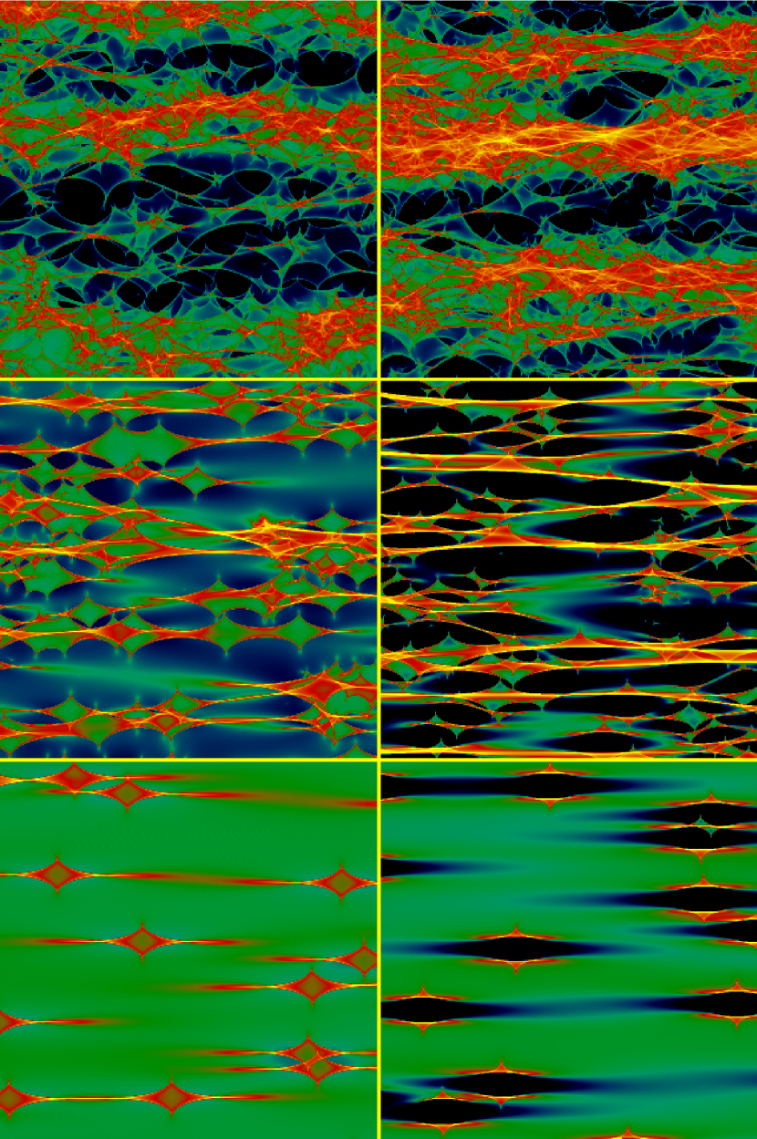
The character of the brightness fluctuations is revealed by mapping the magnification of the source as a function of its position in the source plane (Wambsganss, Paczyński & Schneider 1990). In Figure 2 we show the magnification maps for the “typical” macro-minimum (on the left) and macro-saddlepoint (on the right) with smooth matter fractions of 0%, $\sim 85$% and $\sim 98$%, from top to bottom.

Figure 3 presents magnification histograms computed for each of these. These are the top, middle and bottom panels. In the second and fourth panels we include intermediate histograms for smooth matter fractions $\sim 75$% and $\sim 95$%. For the sake of comparison with our toy model, we discuss the 98% smooth matter model first and proceed to higher densities of microlenses.

Both the magnification maps and the histograms for the 98% smooth matter cases confirm the qualitative results of our toy model. For the macro-minimum, the magnification is mostly just that given by the smooth macro-model. There are isolated diamond shaped caustics that surround “plateaus” of slightly higher magnification which correspond to the 4 micro-image regions described in the toy model. They have one extra micro-minimum. The sharp transitions between the typical magnification and the plateaus are the caustics, marking the points at which a new micro-saddlepoint/micro-minimum pair is created or annihilated. Students of stellar and planetary microlensing will recognize these configurations as the magnification map of a planet lying just outside the Einstein ring of its parent star (Chang and Refsdal 1979, 1984; Mao & Paczyński 1991; Wambsganss 1997).

For the macro-saddlepoint, the magnification is again mostly just that given by the smooth macro-model. But there are occasional “lagoons” of very low magnification, bracketted by small triangular “calderas” of high magnification. The lagoons appear whenever a microlens lies directly along the line of sight. The calderas mark the 4 micro-image regions described in the toy model, and have one extra micro-minimum. The lagoons have no micro-minima. This lagoon/twin-triangle configuration corresponds to the magnification map of a planet inside the Einstein ring of its parent star (Chang and Refsdal 1979, 1984; Wambsganss 1997).

For the 98% (and 95%) cases the histograms for macro-minima and macro-saddlepoints are quite different. Though both are narrow, the saddlepoint histogram is broader and shifted toward high magnifications rather than low magnifications. Moreover it has a very long tail, over the length of which it is quite flat, extending faintward toward unit magnification. It will therefore not be surprising if, with more microlenses, the magnification histogram for the macro-saddlepoint is broader than that for the macro-minimum.

The magnification maps for the 85% cases bear some resemblance to the 98% smooth matter maps, but are far more complex. For the macro-minimum the diamond caustics now begin to overlap, sometimes multiple times, producing successively higher plateaus. The area completely outside the caustics, regions that produce only one micro-minimum, now have clearly lower than average magnification. The corresponding magnification histogram shows two distinct peaks associated with regions of one and two micro-minima (cf. Rauch et al. 1992). In the 75% smooth matter histogram this bifurcation is even more pronounced.

For the macro-saddlepoint the lagoons, regions with no micro-minima, have now grown to the point at which they dominate the magnification map. The triangular calderas have also grown, to the point at which their caustics sometimes cross, producing regions with two, three and four micro-minima. The magnification histogram shows two distinct peaks, corresponding to regions with zero and one micro-minima, respectively, and perhaps a plateau corresponding to regions with two micro-minima. The histogram has a long tail toward high magnifications and drops abruptly very near the minimum magnification allowed by our toy model, $\mu_{\rm tot}=1$. Again, the 75% smooth matter histogram shows a yet more pronounced bifurcation.

In the 0% smooth simulations the macro-minimum and macro-saddlepoint have begun to resemble each other. For the macro-saddlepoint, the low magnification lagoons, still with no micro-minima, have been crowded out by the expanding web of caustics. Most of the magnification map is covered by regions with large numbers of micro-minima. The web of caustics has also expanded for the macro-minimum. The region outside all caustics looks much the same as for the macro-saddlepoint, though these regions still produce one micro-minimum.

We get the general impression that the diamond and lagoon/twin-triangle configurations are the building blocks from which the higher density configurations are constructed. We start out with relatively isolated features. As the surface density of perturbers increases, the fluctuations increase as the building blocks begin to cover the source plane. Increasing the density of perturbers yet further, the building blocks overlap and begin to average out, decreasing the fractional amplitude of the fluctuations.

4.3 Image Magnification $|\mu_{tot}|\sim 25$

Witt et al. (WMS) considered the specific case of MG0414+0534, a quadruple system for which the flux ratio of the close bright pair of images, $A_{2}/A_{1}$, was 0.9 in the radio (Katz and Hewitt 1993) and $0.45\pm 0.06$ in the optical (Schechter and Moore 1993). By contrast their predicted flux ratio was 1.1.

They investigated whether the difference in flux ratios might be due to microlensing, assuming no smoothly distributed matter. Their a posteriori assessment was that the flux difference between the observed optical flux ratio and the predicted ratio is “unlikely, but not ridiculously so.”

We carried out a second suite of simulations, M25 and S25 in Table 1, using the WMS macro-parameters, but adding increasing proportions of smoothly distributed matter, up to 97.5%.

The magnification maps and histograms are similar in broad outline but different in detail from the M10 and S10 models. For the 0% smooth matter case, the caustic networks are very much denser. The histograms for the 0% case are narrower than for models M10 and S10. They are more nearly symmetric and are more similar to each other.

As the smooth matter percentage is increased both histograms widen. The low magnification tail for the macro-saddlepoint drops sharply at $\mu_{\rm tot}\sim 1$, consistent with our toy model. The saddlepoint histogram bifurcates, with the bifurcation most prominent and the distribution broadest for the 93% smooth matter model.

4.4 Lower Limits to the Magnification Histograms

The magnification histograms in Figure 3 show sharp cutoffs at faint magnification. For saddlepoints this corresponds to the minimum magnification in our toy model, equation (5), which approaches unit magnification as $\kappa_{\rm tot}\approx\gamma$ approaches $\text@frac{1}{2}$. For macro-minima the minimum magnification is given by the magnification in the absence of the clumpy component,

$$\mu_{\rm min}={1\over[(1-\kappa_{c})^{2}-\gamma^{2}]}\quad{\rm(minima)}$$ (9)

(cf. Webster et al. 1991). For minima, adding microlenses can only increase the magnification above this value.

4.5 Microlensing in the $\kappa^{\rm eff}-\gamma^{\rm eff}$ Plane

The simulations presented in the preceding subsections trace locii in the $\kappa^{\rm eff}-\gamma^{\rm eff}$ plane appropriate to images with a constant observed magnification and varying proportions of smoothly distributed and microlensing matter. It is worthwhile to consider the results of previous investigations in this framework. Watson and Deguchi (1987, 1988) obtained analytic results along the $\gamma=0$ axis, as did Seitz, Wambsganss and Schneider (1994). Witt, Mao and Schechter (1995) did simulations along the $\gamma=3\kappa-1$ locus. Wambsganss (1992) carried out simulations for several different values of $\gamma$ at $\kappa=0.2$, $0.5$ and $1.5$. Lewis and Irwin (1995) performed simulations on an uneven $5\times 5$ grid covering $0<\kappa<1$, $0<\gamma<1$. They organized their histograms so as to show their coverage of the $\kappa-\gamma$ plane.

Generalizing from the above results, it seems clear that microlensing fluctuations go to zero along the locus of infinite magnification, $\gamma=1-\kappa$, separating minima from saddlepoints. Since they also go to zero along the $\kappa=0$ axis there must be a ridge of maximum fluctuation amplitude (for minima) somewhere in between. There would also appear to be a ridge for saddlepoints which has been crossed by the WMS simulations and also by those in the preceding section. While the presently available coverage of the $\kappa-\gamma$ plane is too sparse to accurately map out this locus, it would seem to coincide, at least roughly, with the $\mu=4$ hyperbola for minima and the $\mu=-3$ hyperbola for saddlepoints. If so then the phenomenon of increasing fluctuations with the addition of smoothly distributed matter is restricted to more highly magnified images.

As is clear from Figures 3 and 4, the rms fluctuation in magnitude is only one of several statistics needed to describe microlensing magnification histograms in anything like their full detail. Their asymmetries vary considerably, and they often bifurcate. We would assign no special physical significance to the locus of maximum rms fluctuation, taking it only to be a convenient measure of variability.

5 MICROLENSING AND MG0414+0534

5.1 The $A_{2}/A_{1}$ Flux Ratio

Witt, Mao and Schechter (1995) present histograms of magnitude differences,

$$\Delta m_{A_{1}/A_{2}}\equiv-2.5\log{A_{1}\over A_{2}}$$ (10)

for three values of the ratio of the Gaussian source radius, $r_{s}$ to the Einstein ring radius $\xi_{E}$. They estimate that the effect of letting $r_{s}/\xi_{E}\rightarrow 0$ would broaden the histogram for $r_{s}/\xi_{E}=0.04$, their smallest value, by an additional 10%.

For the sake of comparison with WMS, we carried out our M25 and S25 simulations using the same convergence and shear, and the same value for the source radius, $r_{s}/\xi_{E}=0.04$. Figure 4 shows $\Delta m_{A_{1}/A_{2}}$ histograms computed for four of our simulations (cases M25 and S25). The first of these, with no smoothly distributed matter, satisfactorily reproduces the WMS histogram, with small differences consistent with differences in the simulation technique. The second, with 87.5% smooth matter, is considerably broader. Moreover, it is asymmetric, with $A_{2}$ more likely to be fainter than $A_{1}$.

The third, for 92.5% smooth matter, shows the broadest distribution. With still increasing fraction of smooth matter, the distributions quickly get narrower again, as the fourth column for 97.5% smooth matter illustrates, though it does show a small plateau.

For the case of 0% smooth matter, the probability that $A_{2}$ will be more than 0.87 magnitudes fainter than $A_{1}$ is 0.068 (cf. WMS). For the 87.5% smooth matter case, that probability has grown to 0.28, and to 0.35 for the 93% smooth matter case, an increase of more than a factor of five. We conclude that if the smoothly distributed matter surface mass density along the line of sight were 87.5% or 92.5% of the total, flux ratios as extreme as that seen in MG0414+0534 would not be uncommon, as long as the saddlepoint image is the fainter of the two images.

5.2 Photometric Dark Matter Fraction

On the assumption that the lensing galaxy in MG0414+0534 is like nearby elliptical galaxies, a dark matter fraction can be derived as follows. Kochanek et al. (2000) measure a deVaucouleurs effective radius for the lensing galaxy of 0$\farcs$78. The Kormendy relation (Kormendy 1977) presented by Bernardi et al. (2001) in their Figure 49 can be used to obtain an expected zero redshift surface brightness. To take advantage of the mass to light ratios presented by Kauffmann et al. (2002) we use the $g^{\prime}$ surface brightness, for which the M/L for a present day elliptical is roughly 4 if $H_{0}$ = 70 km/s/Mpc. The stellar surface mass density is then 386 $M_{\sun}$/pc² at the observed effective radius of the lens, assuming no evolution in the mass profiles of elliptical galaxies.

For an Einstein ring radius of $1\farcs 15$ (Trotter et al. 2000) and a deVaucoulers profile, the stellar surface density is smaller on the ring by a factor of 0.46, giving 177 $M_{\sun}$/pc². For a lens redshift $z_{L}=0.96$ and a source redshift $z_{S}=2.64$ we find a critical surface density of $\Sigma_{c}=2189M_{\sun}$/pc² for $(\Omega_{m},\Lambda)=(0.3,0.7)$. For an isothermal sphere the surface density on the Einstein ring is one half the critical surface density. We therefore have ${\kappa_{*}/\kappa_{\rm tot}=0.16}$ on the Einstein ring, which is the approximate location of the $A_{1}$ and $A_{2}$ images. It is interesting to note that the “best” models of Trotter et al. (2000) give magnifications for the $A_{1}$ and $A_{2}$ images of order $\sim 15$, smaller by $3/5$ than the WMS values. Had Witt et al. adopted a model in which the quadrupole moment was due to flattening of the galaxy rather than an external tide, they would have found magnifications smaller by $\sim 1/2$, making our S10 and M10 models more appropriate.

5.3 Smoothly Distributed Matter and Source Size

Witt Mao and Schechter (1995) obtained a 95% confidence upper limit on the source size for MG0414+0534 of $10^{16}$ cm $\times(<M>/0.1M_{\sun})^{1/2}$ for the case of no smoothly distributed matter. As increasing the smooth matter content increases the fluctuation amplitude, that upper limit on the source size is relaxed.

Most simulations of microlensing use a finite source size, parameterized by $r_{s}/\xi_{E}$. This adds a third dimension to one’s model space. A rough idea of the effect of source size can be had by taking the source to be composed of two components – one very compact, so that point source simulations suffice, and one very extended, so that the macro-magnification holds. The resulting magnification map is then just a luminosity weighted average of a point source map and a uniform map.

The effect of increasing the extended fraction of a source is to compress the magnification histograms of Figure 3 horizontally, preserving their shapes. Thus while increasing the extended fraction of the source would, for bright images, mimic decreasing the smoothly distributed fraction of the lens, details of the magnification histograms will be different and residuals from an ensemble of identical systems would in principal permit further tighter constraints on both the smoothly distributed mass fraction and the extended source fraction. The source and lens in MG0414+0534 are surely moving with respect to each other. If we wait long enough, we will get a new, statistically independent set of flux ratios.

5.4 Alternative Interpretations

Many gravitationally lensed systems have images with different observed colors. This could be a natural consequence of microlensing under the assumption that the optical emission arises from an accretion disk whose size is roughly that of the microlenses. Blue flux coming from the inner part of the accretion disk would therefore be more vulnerable to microlensing than red flux coming from further out. This would result in larger fluctuations (i.e. flux ratios) at shorter wavelengths (Wambsganss and Paczyński 1991). In the case of MG0414+0534, one might expect the blue flux to be more heavily suppressed than the red flux. In fact the $A_{2}/A_{1}$ flux ratio observed at 2.05 µm  is considerably closer to unity than that observed at 0.8 µm.

But dust in the intervening galaxy might also give rise to such an effect. Assuming that the color differences are due to dust in the intervening galaxy, Falco et al. (1999) have used them to derive corrected flux ratios, reducing all images to a common residual extinction. Adopting a standard extinction curve they derive an extinction corrected $A_{2}/A_{1}=1.05$. But Falco et al. call the lensing galaxy an elliptical galaxy, and elsewhere the same authors treat the lensing galaxy as elliptical (as most lenses are) including it in their study of the fundamental plane of lensing galaxies (Kochanek et al. 2000). It seems unlikely to the present authors that an E3 elliptical galaxy would have a single spot of dust with 1 magnitude of extinction at $1.5r_{e}$, but as we are extrapolating from our experience at $z=0$ to $z=0.96$, we cannot be absolutely certain that we are seeing the effects of microlensing and not dust.

6 THE SMOOTH MATTER FRACTION AS DETERMINED FROM ENSEMBLES

One could in principal measure the smoothly distributed matter content of a single lens by sampling the magnification histograms many times, waiting for the source and lens to move with respect to each other, given a macro-model with accurate values of the shear and convergence. As this could be inconvenient, an alternative would be to assemble an ensemble of lenses and to look at the distribution of intensity ratio residuals from best fitting models. Several surveys for lenses are underway that might produce such samples. In particular the Hamburg-ESO survey (Wisotzki et al. 1996) and the Sloan Digital Sky Survey (Schneider et al. 2002) will ultimately yield large number of lenses.

6.1 Point Sources

The treatment of an ensemble of lenses is most straightforward in the limit where $r_{s}/\xi_{E}$ is small. For every image in every quadruple in the sample, one would obtain a model (ideally not using the flux ratios as constraints) and compute magnification histograms for each of the four images for a range of values of $\kappa_{c}/\kappa_{tot}$. One would then construct a likelihood function from the product of the probabilities obtained from the histogram. There would be an additional free parameter for each system – a number which converts observed flux into magnification. Maximizing the likelihood would give a best value for the smoothly distributed mass fraction, $\kappa_{c}/\kappa_{tot}$.

The number of systems needed to establish the presence of smoothly distributed matter need not be large. From the histograms in Figure 3 we see that a single system with a saddlepoint 2 magnitudes fainter than predicted would rule out the 0% smooth case at the $2\sigma$ level.

A variant of this approach would be to assign a range of mass-to-light ratios to the observed surface brightness profile for each lensing galaxy, attributing the shortfall in surface density to smoothly distributed matter.

6.2 Finite Sources

There are both theoretical and observational reasons to think that $r_{s}/\xi_{E}$ is not vanishingly small, at least for some systems. The one-size-fits-all approach would be to assign a single value of $r_{s}/\xi_{E}$ to every system (or a fixed physical size $r_{s}$, scaled properly by the lens-dependent $\xi_{E}$), and then maximize the likelihood function with this additional variable. One might use a Gaussian surface brightness profile for the sources or, for the sake of computational speed, treat the quasar as a point source embedded in a very extended source. More realistically, but at the cost of considerable additional complexity, one could allow each system to have a different (e.g., luminosity-dependent) source size and profile.

6.3 Double Image Systems

We have emphasized quadruple systems rather than doubles because the effects of smoothly distributed matter would seem to be more important at high magnifications. The results of the previous sections would indicate that even doubles that are not highly magnified could still suffer substantial microlensing.

However, doubles suffer from another difficulty – a dearth of model constraints. One needs 5 constraints to obtain the simplest SIS with external shear model, and doubles have only four positional constraints – the two image positions relative to the lens. The flux ratio is often taken as the fifth constraint, but using it as a constraint will give a perfect fit to the model. Doubles are not beyond redemption, however; one might use radio flux ratios, emission line ratios (Wisotzki et al. 1993), or mid-IR flux ratios (Agol et al. 2000) to constrain the model on the hypothesis that the emission regions are large compared to the Einstein rings of the microlenses.

7 FURTHER CONSEQUENCES

7.1 Millilensing and Mini-halos

The present work is fundamentally similar to (though on the surface quite different from) that of Metcalf and Madau (2001), Chiba (2002) and Dalal and Kochanek (2002) who argue that the brightness ratio anomalies observed in quadruple systems are due to the presence of dark matter mini-halos.

The differences are obvious. They substitute increasing amounts of clumpy dark matter for smoothly distributed luminous matter. We substitute increasing amounts of smoothly distributed “dark” matter for clumpy luminous matter. But the phenomenon we seek to explain is the same.

We find, as they do, that a small micro- (or milli-) lensing fraction produces surprisingly large flux ratio anomalies. In our case we find this to be especially true for saddlepoints.

But the situation for extended micro- or millilenses is somewhat different than for point mass perturbers. If we follow the same line of reasoning as in our toy model, but taking the perturbers to be singular isothermal spheres directly along the line of sight to the macro-images, we find that both the micro-minima and micro-saddlepoints have twice the magnification that the corresponding point mass perturber would have had. In the limit as $\gamma\approx\kappa_{tot}\rightarrow\text@frac{1}{2}$, the SIS perturber doubles the magnification of a macro-minimum and reduces the macro-saddlepoint but still leaves it a factor of two brighter than the unmagnified source. We therefore expect extended perturbers to produce larger fluctuations for macro-minima and smaller fluctuations for macro-saddlepoints than would point mass perturbers. The anomalies ought to be more uniformly distributed among the multiple images, and not so heavily weighted toward the saddlepoints. Perhaps this is why Dalal and Kochanek (2002) made no distinction among macro-minima and macro-saddlepoints in their discussion (though they appear to have treated these correctly in their simulations). Metcalf and Madau (2001) do note an asymmetry between the two, and their figures show it to be in the same sense, if not as exaggerated, as those we find for point perturbers.

Dalal and Kochanek (2002) argue that the anomalous flux ratios observed at radio wavelengths are due to millilensing by subhalos comprised entirely of dark matter. This rests on the fact that radio sources are larger than the Einstein rings of individual stars. Metcalf and Zhao (2001), building on the work of Metcalf & Madau (2001), argue for a similar effect including optical as well as radio fluctuations in their discussion.

If radio emission regions in quasars were small compared to the Einstein rings of the stars in the lensing galaxies, the results of the previous sections would undermine the conclusions regarding subhalos, since some fraction of the observed fluctuations would be due to micro- rather than millilensing.

7.2 Millilensing vs. Microlensing

In fact, there is a way to distinguish microlensing effects that we propose here as an explanation for the discrepant intensity ratios in close double images, from millilensing, as suggested by Mao & Schneider (1998), Metcalf & Madau (2001), Metcalf & Zhao (2001), or Dalal & Kochanek (2002). Since quasar, lensing galaxy and observer move relative to each other, the brightness of one particular quasar image will change with time due to the fact that the focussing matter in front of it changes position. The time scale of such fluctuations is of order a few years up to a decade for microlensing by solar-mass stars. Since this timescale is proportional to the Einstein radius of the lenses, it increases with the square root of the mass of the lensing objects. Typical masses of substructure clumps range from about $10^{2}M_{\odot}$ to $10^{6-9}M_{\odot}$ (Metcalf & Madau 2001, Dalal & Kochanek 2002). This means millilensing effects of such substructure clumps should not modify the intensity ratios of affected multiple-quasars over the professional lifetime of an astronomer, whereas microlensing should produce variable intensity ratios.

7.3 Modelling Lenses

The magnification histograms presented in Figures 3 and 4 show that flux ratios are reliable constraints only in the absence of micro- and millilensing. If either is suspected, one will want to take the expected fluctuations into account. Since the histograms can be quite broad and heavily skewed, proper treatment demands a full-blown maximum likelihood analysis rather than the assumption of Gaussian residuals. Fitting for fluxes should work better than fitting for magnitudes (i.e., log flux), since the mean magnitude residuals can be quite different from zero.

7.4 Non-isothermality: Is Smoothly Distributed Matter Necessary?

The singular isothermal sphere model discussed here is the “industry standard” for microlensing. External evidence from the dynamics of nearby elliptical galaxies (Romanowsky and Kochanek 1999) and internal evidence from lensed systems with multiple and extended sources (Kochanek 1995; Bernstein and Fischer 1999; Cohn et al. 2001; Rusin et al. 2002) consistently give potentials with logarithmic slopes very nearly that of an isothermal sphere.

It should be noted, however, that we can also obtain larger fluctuation amplitudes for the bright pairs of images without smoothly distributed matter, by going to models with stars alone that have $\kappa_{*}$ and $\gamma$ equal to our effective convergences and shears. Witt, Mao and Schechter (1995) obtained macro-models for a more centrally concentrated potential midway between a singular isothermal sphere and a point mass (parameterized by setting their $\beta=1/2$). This comes close to what one might expect for a deVaucouleurs $r^{1/4}$ profile at constant mass to light ratio.

The magnifications are then smaller by roughly a factor of two than for their isothermal models. For MG0414+0534, the $\beta=1/2$ model gives convergences and shears for the bright pair of images of (0.229,0.710) and (0.239,0.814), respectively, for the $A_{1}$ minimum and $A_{2}$ sadddlepoint. The isothermal model, with $\kappa_{*}/\kappa_{\rm tot}=0.333$, would give an effective convergence and shear of (0.230,0.712) and (0.239, 0.813), making the two fluctuation histograms virtually indistinguishable.

If a very long sequence of observations ruled out $\kappa_{*}/\kappa_{\rm tot}=0.333$ for the isothermal model, it would also rule out the $\beta=1/2$ model. At least in principle, then, fluctuation observations might rule out constant mass to light ratios.

Taken alone, the qualitative aspects of anomalous flux ratios, and in particular suppressed saddlepoints, cannot establish the presence of a dark component. But to the extent that other techniques do demonstrate the presence of a dark component, anomalies can establish that this dark component must be smooth.

8 SUMMARY AND CONCLUSIONS

We have shown that the substitution of a smoothly distributed matter component for the clumpy stellar surface density increases rather than decreases the amplitude of microlensing brightness fluctuations for close pairs of images in quadruple gravitational lenses. We have also shown that in the presence of a smoothly distributed component, the magnification probabily distributions for saddlepoints and minima of the Fermat arrival time surface are quite different, making it likely that saddlepoints undergo substantial demagnification. Inclusion of a smoothly distributed matter component in models for MG0414+0534 makes the large optical flux ratio of the bright pair of images considerably more likely under the microlensing hypothesis.

In extreme cases a single flux ratio anomaly might serve to establish the relative proportions of smooth and microlensing mass. More generally the relative contribution of smoothly distributed matter may be established either by observing an ensemble of lensed systems or by carrying out a (long) time series for a single system.

Figure 1: $\kappa^{\rm eff}$-$\gamma^{\rm eff}$-plane. Images corresponding to minima in the arrival time surface form in the hatched region; maxima form in the cross-hatched region; saddlepoint images form in the remaining triangular region. Lines of constant magnification are hyperbolae. The symbols indicate the models we investigated (M10 – squares; S10 – stars). The symbols approach the vertical axis as increasing amounts of smoothly distributed matter are substituted for microlensing matter, keeping $\kappa_{tot}$ constant.

Figure 2: Two-dimensional microlensing magnification distribution in the quasar plane, for a minimum (left, models M10) and a saddlepoint image (right, models S10). The color scale ranges from dark blue (large demagnification) - light blue - green - red - yellow (large magnification). The total convergence $\kappa_{tot}$ remains constant for each column, whereas the fraction of smoothly distributed matter increases downward from 0% at the top through 85% in the middle to 98% at the bottom (corresponding to rows 1, 3 and 5 of Figure 3).

Figure 3: Magnification probability distribution for a minimum (left, models M10, $\gamma=0.425$) and a saddlepoint image (right, models S10, $\gamma=0.575$). The total convergence $\kappa_{tot}$ remains constant for each column. The smoothly distributed matter increases from top to bottom, with fractional contributions of 0%, 75%, 85%, 95% and 98%, respectively. The three vertical lines indicate the following: short-dashed: $\Delta m=0$ mag (theoretically expected macro-magnification); dotted: $<\Delta m>$ (average magnification in magnitudes); long-dashed: $\mu_{\rm abs}=1.0$ (absolute magnification unity, i.e. unlensed case).

Figure 4: Probability distributions for the magnitude difference between images A₁ and A₂ of MG0414+0534, with parameters as chosen by WMS: $\kappa_{\rm A_{1},tot}=0.472$, $\gamma_{\rm A_{1}}=0.488$ (our model M25), and $\kappa_{\rm A_{2},tot}=0.485$, $\gamma_{\rm A_{2}}=0.550$ (our model S25). Column 1 illustrates the case of all matter in clumpy form (same as treated in Figure 4 of WMS); the panel at the top shows the differential probability, the bottom panel presents the corresponding integrated probability. Columns 2, 3 and 4 show the corresponding probability distributions for 88.5% smooth matter, 93% smooth matter, and 97.5% smooth matter, respectively.

References

- (1) Agol, E., Jones, B., & Blaes, O. 2000, ApJ, 545, 657
- (2) Bernardi, M. et al. 2001, preprint (astro-ph/0110344)
- Bernstein & Fischer (1999) Bernstein, G. & Fischer, P. 1999, AJ, 118, 14
- (4) Blandford, R. D. & Narayan, R. 1986, ApJ 310, 568
- (5) Chang, K. & Refsdal, S. 1979, Nature, 282, 561
- (6) Chang, K. & Refsdal, S. 1984, A&A, 132, 168
- Chiba (2002) Chiba, M. 2002, ApJ, 565, 17
- Cohn, Kochanek, McLeod, & Keeton (2001) Cohn, J. D., Kochanek, C. S., McLeod, B. A., & Keeton, C. R. 2001, ApJ, 554, 1216
- Dalal & Kochanek (2002) Dalal, N. & Kochanek, C. S. 2002, ApJ, 572, 25
- (10) Deguchi, S. & Watson, W. D. 1987, PRL 59, 2814
- (11) Deguchi, S. & Watson, W. D. 1988, ApJ 335, 67
- Falco et al. (1999) Falco, E. E. et al. 1999, ApJ, 523, 617
- (13) Gaudi, B. S. & Petters, A. O. 2002, ApJ 574, 970
- (14) Hewitt, J. N., Turner, E. L., Lawrence, C. R., Schneider, D. P. & Brody, J. P. 1992, AJ 104, 968
- (15) Kayser, R., Refsdal, S. & Stabell, R. 1986, A&A 166, 36
- (16) Katz, C. A. & Hewitt, J. N. 1993, ApJ 409, L9
- (17) Kauffmann, G. et al. 2002, preprint (astro-ph/0204055)
- (18) Kochanek, C. S. 2002, preprint (astro-ph/0204043)
- Kochanek (1995) Kochanek, C. S. 1995, ApJ, 445, 559
- Kochanek et al. (2000) Kochanek, C. S. et al. 2000, ApJ, 543, 131
- Kormendy (1977) Kormendy, J. 1977, ApJ, 218, 333
- (22) Lawrence, C. R., Elston, R., Januzzi, B. T., & Turner, E. L. 1995, ApJ, 110, 2570.
- (23) Lewis, G. F. & Irwin, M. J. 1995, MNRAS 276, 103
- (24) Lewis, G. F. & Irwin, M. J. 1996, MNRAS 283, 225
- (25) Lewis, G. F., Miralda-Escudé, J., Richardson, D. C. & Wambsganss, J. 1993, MNRAS 261, 647
- (26) Mao, S. & Paczyński, B. 1991, ApJ 374, L37
- (27) Mao, S. & Schneider, P. 1998, MNRAS 295, 587
- (28) Metcalf, R. B. & Madau, P. 2001, ApJ 563, 9
- (29) Metcalf, R. B. & Zhao, H. 2001, ApJL 456, L5
- (30) Paczyński, B. 1986, ApJ 301, 503
- (31) Rauch, K.P., Mao, S., Wambsganss, J. & Paczyński, B. 1992, ApJ 386, 30
- (32) Refsdal, S. & Surdej, J. 1994, Rep. on Progr. Phys. 56, 117
- (33) Reimers, D., Hagen, H. J., Baade, R., Lopez, S. & Tytler, T. 2002, A&A, 382, L26
- Romanowsky & Kochanek (1999) Romanowsky, A. J. & Kochanek, C. S. 1999, ApJ, 516, 18
- Rusin et al. (2002) Rusin, D., Norbury, M., Biggs, A. D., Marlow, D. R., Jackson, N. J., Browne, I. W. A., Wilkinson, P. N., & Myers, S. T. 2002, MNRAS, 330, 205
- Saha (2000) Saha, P. 2000, AJ, 120, 1654
- (37) Schechter, P. L. & Moore, C. B. 1993, AJ 105, 1
- (38) Schneider, D. P. et al. 2002, AJ, 123, 567
- (39) Schneider, P. & Weiss, A. 1987, A&A 171, 49
- (40) Seitz, C. & Schneider, P. 1994, A&A 288, 1
- (41) Seitz, C., Wambsganss, J. & Schneider, P. 1994, A&A 288, 19
- (42) Trotter, C. S., Winn, J. N. & Hewitt, J. N. 2000, ApJ 535, 671
- (43) Wambsganss, J. 1990, PhD Thesis, Report MPA550
- (44) Wambsganss, J. 1992, ApJ 386, 19
- (45) Wambsganss, J. 1997, MNRAS 284, 172
- Wambsganss & Paczynski (1991) Wambsganss, J. & Paczyński, B. 1991, AJ, 102, 864
- (47) Wambsganss, J., Witt, H. J. & Schneider, P. 1992, A&A 258, 591
- (48) Wambsganss, J., Paczyński B. & Schneider, P. 1990, ApJ 358, L33
- Webster, Ferguson, Corrigan, & Irwin (1991) Webster, R. L., Ferguson, A. M. N., Corrigan, R. T., & Irwin, M. J. 1991, AJ, 102, 1939
- (50) Wisotzki, L., Köhler, T., Kayser, R. & Reimers, D. 1993, A&A 278, L15
- (51) Wisotzki, L., Köhler, T., Groote, D., & Reimers, D. 1996, A&A, 115, 227
- (52) Witt, H. J. 1993, ApJ 403, 530
- (53) Witt, H. J., Mao, S. & Schechter, P. L. 1995, ApJ 443, 18 (WMS)
- (54) Wucknitz, O. 2002, MNRAS 332, 951