Lensing Properties of Cored Galaxy Models

Abstract

A method is developed to evaluate the magnifications of the images of galaxies with lensing potentials stratified on similar concentric ellipses. In a quadruplet system, there are two even parity images, two odd parity images, together with a de-magnified and usually missing central image. A simple contour integral is provided which enables the sums of the magnifications of the even parity or the odd parity images or the central image to be separately calculated without explicit solution of the lens equation. We find that the sums for pairs of images generally vary considerably with the position of the source, while the signed sums of the two pairs can be remarkably uniform inside the tangential caustic in the absence of naked cusps.

For a family of models in which the lensing potential is a power-law of the elliptic radius, $\psi\propto(a^{2}+x^{2}+y^{2}q^{-2})^{\beta/2}$, the number of visible images is found as a function of flattening $q$, external shear $\gamma$ and core radius $a$. The magnification of the central image depends on the size of the core and the slope $\beta$ of the gravitational potential. It grows strongly with the source offset if $\beta>1$, but weakly if $\beta<1$. For typical source and lens redshifts, the missing central image leads to strong constraints; the slope $\beta$ must be $\mathrel{\hbox to0.0pt{\lower 3.0pt\hbox{$\sim$}\hss}\raise 2.0pt\hbox{$<$}}1$ and the core radius $a$ must be $\mathrel{\hbox to0.0pt{\lower 3.0pt\hbox{$\sim$}\hss}\raise 2.0pt\hbox{$<$}}300$ pc. The mass distribution in the lensing galaxy population must be nearly cusped, and the cusp must be isothermal or stronger. This is in good accord with the cuspy cores seen in high resolution photometry of nearby, massive, early-type galaxies, which typically have $\beta\approx 0.7$ (or surface density falling like distance^-1.3) outside a break radius of a few hundred parsecs. Cuspy cores by themselves can provide the explanation of the missing central images. Dark matter at large radii may alter the slope of the projected density; however, provided the slope remains isothermal or steeper and the break radius remains small, then the central image remains unobservable. The sensitivity of the radio maps must be increased fifty-fold to find the central images in abundance.

1 Introduction

For smooth, non-singular lenses, it is well-known that the total number of images is odd and that the number of even parity images exceeds the number of odd parity images by one (e.g., Burke 1981; Schneider, Ehlers & Falco 1992, chap. 5). When the source lies within both the tangential and radial caustics, it is lensed into 5 images. When the source lies outside one caustic but inside the other, then it is lensed into 3 images. If the surface density at the galaxy centre is cusped and that cusp is stronger than isothermal, then the situation changes. There is no radial caustic and there are either 4 or 2 images depending on whether the source lies inside or outside the remaining tangential caustic (Evans & Wilkinson 1998).

In fact, almost all the known sixty or so gravitational lens systems are 2 or 4 image configurations (see Pospieszalka et al. 1999 for details of the gravitational lensing database which maintains a list of candidates). There are two systems in which the presence of a weak, central image has been claimed. APM08279+5255 is an ultraluminous broad absorption line quasar. Originally, two images were detected serendipitously by Irwin et al. (1998) in the optical. Subsequently, Ibata et al. (1999) found convincing evidence for a central third image using higher resolution infrared imaging. The source of MG1131+0456 is a radio galaxy. One extended radio component is lensed into a ring, another is lensed into two images. There seems to be a weak central image at the center of the ring, and this may be the third or fifth image of parts of the background radio source (Chen & Hewitt 1993); however, this could also be emission from the lensing galaxy. The almost total absence of the central image from the known lens systems sets strong constraints on the core radius and the steepness of the lensing potential (e.g., Narayan, Blandford & Nityananda 1984, Wallington & Narayan 1993, Rusin & Ma 2000).

The aims of this paper are twofold. On the theoretical side, our aim is to find expressions for the sums of the magnifications of any subset of the images produced by multiply lensed quasars or galaxies, at least within the framework of a class of flexible and popular models. We do this by extending the analysis of our earlier work (Hunter & Evans 2001, henceforth Paper I) to lensing potentials stratified on similar concentric ellipse but this time with cores. In doublet (or quadruplet) systems, there are one (or two) even parity images, one (or two) odd parity images, together with the missing central image. We provide contour integrals which find the sums of the magnifications of the even parity images, the odd parity images and the central image separately. On the astrophysical side, our aim is to set constraints on the cusp profile and core size of lensing galaxies by requiring that the central image be too weak to be detectable. For the 2 and 4 image systems, we investigate the permissible core radius as a function of the steepness and the flattening of the lensing potential and the external shear.

The paper is arranged as follows. Section 2 develops the contour integral representation needed for lensing potentials that are elliptically stratified. Section 3 specialises the analysis to models in which the lensing potential is a power-law of the elliptic radius combined with external shear of arbitrary orientation. The conditions for triple and quintuple imaging are found in terms of the depth and shape of the potential, as well as the position of the source. The contour integrals for the sums of the magnifications of the two even parity, the two odd parity and the missing central image are evaluated. Section 4 uses Monte Carlo simulations to set limits on the lensing potential by requiring the central image to be unobservable. Finally, our conclusions are given in Section 5.

2 Contour Integrals for Observables

This section develops contour integrals for computing the magnifications of images assuming only that the lensing potential is stratified on similar concentric ellipses.

2.1 The Lens Equation

In this paper, we always assume that the lensing potential $\psi$ is stratified on similar concentric ellipses with constant axis ratio $q$ with $0<q\leq 1$ so that

$$\psi=\psi(\tau),\qquad\qquad\tau=x^{2}+y^{2}q^{-2}.$$ (1)

For a thin lens with potential $\psi$, the lens equation is (e.g., Schneider et al., section 5.1)

$$\xi=x+\gamma_{1}x+\gamma_{2}y-2x\psi^{\prime}(\tau),\qquad\eta=y+\gamma_{2}x-\gamma_{1}y-{2y\over q^{2}}\psi^{\prime}(\tau),$$ (2)

where ($\xi,\eta$) are Cartesian coordinates of the source. Here $\gamma_{1}$ and $\gamma_{2}$ allow for a constant external shear in an arbitrary direction. We always assume that the lens is not circularly symmetric (that is, either $q\neq 1$ or $\gamma_{1}\neq 0$ or $\gamma_{2}\neq 0$).

Complex numbers often simplify calculations in lensing theory (e.g., Bourassa, Kantowski & Norton 1973, Bourassa & Kantowski 1975, Witt 1990, Rhie 1997). As in Paper I, we shall find it helpful to use

$$\zeta=\xi+{\rm i}q\eta=|\zeta|e^{i\phi},\qquad\qquad z=x+{\rm i}y/q,\qquad\qquad\tau=z{\bar{z}}.$$ (3)

The lens equation (2) then becomes

$$\zeta=P_{0}z+Q{\bar{z}}-2z\psi^{\prime}(\tau),$$ (4)

where

$$P_{0}={\textstyle\frac{1}{2}}[1+q^{2}+\gamma_{1}(1-q^{2})],\qquad Q={\textstyle\frac{1}{2}}[1-q^{2}+\gamma_{1}(1+q^{2})+2{\rm i}q\gamma_{2}].$$ (5)

It and its conjugate can be written in matrix form as

$$\left(\begin{array}[]{l}\zeta\\ {\bar{\zeta}}\\ \end{array}\right)=\left(\begin{array}[]{lr}P&Q\\ {\bar{Q}}&P\\ \end{array}\right)\left(\begin{array}[]{l}z\\ {\bar{z}}\\ \end{array}\right),$$ (6)

where $P=P_{0}-2\psi^{\prime}(\tau)$, from which it follows that

$$\left(\begin{array}[]{l}z\\ {\bar{z}}\\ \end{array}\right)={1\over P^{2}-|Q|^{2}}\left(\begin{array}[]{lr}P&-Q\\ -{\bar{Q}}&P\\ \end{array}\right)\left(\begin{array}[]{l}\zeta\\ {\bar{\zeta}}\\ \end{array}\right).$$ (7)

When we form the real quantity $\tau=z{\bar{z}}$ from eqn. (7), we find that the solutions of the lens equation also satisfy the real equation

$$K(\tau;\zeta,{\bar{\zeta}})\doteq{1\over\tau}(P\zeta-Q{\bar{\zeta}})(P{\bar{\zeta}}-{\bar{Q}}\zeta)-\left[P^{2}-|Q|^{2}\right]^{2}=0.$$ (8)

We designate $K(\tau;\zeta,{\bar{\zeta}})=0$ as the imaging equation. Its real and positive solutions for $\tau$ provide the image positions $z$ for a given source location $\zeta$. Once a solution for $\tau$ is found, the image positions are given by equation (7). Any solution of the original lens equation (2) gives a solution of the imaging equation. However, the imaging equation may have negative real or complex solutions which do not correspond to true images.

2.2 Sums of Magnifications

The lens equation defines a map from the complex $(z,{\bar{z}})$–lens plane to the $(\zeta,{\bar{\zeta}})$–source plane. The Jacobian of this mapping is

$$J=\left(\begin{array}[]{lr}{\displaystyle\partial\zeta\over\displaystyle\partial z}\Bigl{|}_{\bar{z}}&{\displaystyle\partial\zeta\over\displaystyle\partial{\bar{z}}}\Bigl{|}_{z}\\ {\displaystyle\partial{\bar{\zeta}}\over\displaystyle\partial z}\Bigl{|}_{\bar{z}}&{\displaystyle\partial{\bar{\zeta}}\over\displaystyle\partial{\bar{z}}}\Bigl{|}_{z}\end{array}\right)=\left(\begin{array}[]{lr}P+\tau P^{\prime}({\tau})&Q+z^{2}P^{\prime}({\tau})\\ {\bar{Q}}+{\bar{z}}^{2}P^{\prime}({\tau})&P+\tau P^{\prime}({\tau})\\ \end{array}\right),$$ (9)

where the second form has been evaluated using eqn (6). The eigenvalues and eigenvectors of $J$ determine the distortion of images. If the eigenvalues are both positive, the image is direct; if the eigenvalues are both negative, the image is doubly inverted. These are the even parity cases. If one eigenvalue is positive, the other negative, then the image is inverted and the parity is odd. The reciprocal of the determinant of the Jacobian of the mapping from the real $(x,y)$–lens plane to the $(\xi,\eta)$–source plane corresponds physically to the signed magnification of an image (Schneider et al. 1992, chapter 5). With our choice (3) of complex coordinates, we find

$${q^{2}\over{\rm det}J}\Biggl{|}_{x_{i},y_{i}}=\mu_{i}p_{i},$$ (10)

where $\mu_{i}$ is the absolute value of the magnification and $p_{i}$ is the parity of the image located at $(x_{i},y_{i})$. For certain positions, ${\rm det}J$ vanishes and the magnification is infinite. These are the critical points and lines. The caustics are the images of the critical points and curves under the lens mapping (2). Evaluating the determinant of (9) gives

$${\rm det}J=P^{2}-|Q|^{2}+(2\tau P-Q{\bar{z}}^{2}-{\bar{Q}}z^{2})P^{\prime}({\tau}).$$ (11)

Differentiating the imaging equation (8) for $K$ partially with respect to $\tau$, holding $\zeta$ and ${\bar{\zeta}}$ fixed, and then using the lens equation (6) to express $\zeta$ and ${\bar{\zeta}}$ in terms of $z$ and ${\bar{z}}$ gives

$${\displaystyle\partial K(\tau;\zeta,{\bar{\zeta}})\over\displaystyle\partial\tau}\Bigl{|}_{\zeta,{\bar{\zeta}}}={-(P^{2}-|Q|^{2})\over\tau}\left[P^{2}-|Q|^{2}+(2\tau P-Q{\bar{z}}^{2}-{\bar{Q}}z^{2})P^{\prime}({\tau})\right].$$ (12)

Consequently, we get the following compact expression for the signed magnification of an image as

$$\mu p={q^{2}\over{\rm det}J}={-q^{2}(P^{2}-|Q|^{2})\over\tau{\displaystyle\partial K\over\displaystyle\partial\tau}\Bigl{|}_{\zeta,{\bar{\zeta}}}}.$$ (13)

Our contour integral representation relies on the special structure of equation (13). Images correspond to simple zeros of $K(\tau;\zeta,{\bar{\zeta}})$ and $1/(\partial K/\partial\tau)$ is the residue of $1/K$ at a simple zero. We continue the right hand side of equation (13) into the complex $\tau$-plane and write the sum of the signed magnifications of the images as the contour integral

$$\sum_{{\rm images}}\mu_{i}p_{i}={-q^{2}\over 2\pi{\rm i}}\oint_{\cal C}{d\tau\over\tau}{(P^{2}-|Q|^{2})\over K(\tau;\zeta,{\bar{\zeta}})}.$$ (14)

Here, ${\cal C}$ is a contour in the complex $\tau$-plane which excludes $\tau=0$ and encloses only the simple poles corresponding to whichever visible images we wish to analyse.

Let us note that our analysis here shows how the methods first developed in Paper I can do more than we achieved there. We here exploit them in two new ways. We first relax the restriction that the lensing potential be scale-free and allow it to have a core. Cored potentials produce either one, three, or five images depending on the strength of the potential, the size of the core and the position of the source. Second, we derive formulae for sums of signed magnifications for separate image pairs, and for the central image. Hence, the present results are more detailed and informative than those of Paper I, most of which were for sums over the four bright images, consisting of two pairs of opposite parity, and which therefore partially cancel.

3 Power-Law Galaxies with Cores

We now specialize the analysis to the case of power-law galaxies with a core radius $a$, which have the lensing potential

$$\psi=\left\{\begin{array}[]{ll}{\displaystyle A\over\displaystyle\beta}(a^{2}+\tau)^{\beta/2}&\mbox{if $0<\beta<2$},\\ \hbox{}&\hbox{}\\ {\displaystyle A\over\displaystyle 2}\ln(a^{2}+\tau)&\mbox{ if $\beta=0$}.\end{array}\right.$$ (18)

These models were first studied by Blandford & Kochanek (1989) in the context of gravitational lensing (see also Kassiola & Kovner 1993; Witt 1996; Witt & Mao 1997, 2000; Evans & Wilkinson 1998 and Paper I). They are the projections of three-dimensional power-law galaxies familiar in galactic astronomy and dynamics (Evans 1993, 1994). For example, they have been used to model the nearby elliptical galaxy M32 (van der Marel et al. 1994), the inner parts of the Galactic bulge (Evans & de Zeeuw 1994), as well as the dark halo of our own Galaxy in the interpretation of both the Sagittarius stream and the microlensing results (Alcock et al. 1997; Ibata & Lewis 1998). The convergence (or surface density in units of the critical density) is

$$\kappa={A\over 2q^{2}}\,{a^{2}(1\!+\!q^{2})+x^{2}(1\!+\!q^{2}(\beta\!-\!1))+y^{2}(1\!+\!q^{-2}(\beta\!-\!1))\over(a^{2}+\tau)^{2-\beta/2}}.$$ (19)

It is easy to see that

$$2\psi^{\prime}(\tau)=A(a^{2}+\tau)^{-1/B},$$ (20)

where the parameter $B=2/(2-\beta)$ and has the range $1\leq B<\infty$. The positive parameter $A$, to which the magnitude of the lensing potential is proportional, can be removed by a rescaling. Specifically, we scale all lengths by $A^{B/2}$. The net effect is to set $A=1$ in eqs (18)-(20). The dependence of our results on $A$, which is needed in applications, can be recovered by multiplying all powers of $a$, $z$ and $\zeta$ and their conjugates by the same powers of $A^{B/2}$.

3.1 Images and Caustics

In this section, we establish the conditions for the numbers and types of images, and the forms of the caustics. It is convenient to use the variable $t=(a^{2}+\tau)^{-1/B}$. It reduces to the same variable $t$ used in Paper I in the limit of no core ($a\to 0$). When there is a core, the physically relevant range of $t$ is restricted to $0<t\leq a^{-2/B}$. In terms of the variable $t$,

$${1\over\tau}={t^{B}\over 1-a^{2}t^{B}},\qquad 2\psi^{\prime}(\tau)=t,\qquad P=P_{0}-t.$$ (21)

The imaging equation (8) requires the balance

$${t^{B}(P\zeta-Q{\bar{\zeta}})(P{\bar{\zeta}}-{\bar{Q}}\zeta)\over 1-a^{2}t^{B}}=(P^{2}-|Q|^{2})^{2}=(t-t_{1})^{2}(t-t_{2})^{2},$$ (22)

for those real and positive values of $t$ at which the images occur. The values of $t_{1}$ and $t_{2}$ depend only on the flattening and the shear, and are defined by

$$t_{1}=P_{0}+|Q|,\qquad t_{2}=P_{0}-|Q|.$$ (23)

It follows from the definitions (5) that $P_{0}>0$ and $P^{2}_{0}-|Q|^{2}=q^{2}(1-\gamma^{2}_{1}-\gamma^{2}_{2})>0$ provided that $\gamma_{1}^{2}+\gamma_{2}^{2}<1$. Hence, both $t_{1}$ and $t_{2}$ are positive with $t_{1}>t_{2}$ and $t_{2}<1$. Fig. 1 shows how image positions can be found graphically by plotting separately the two sides of equation (22). The full curve represents the right hand side of that equation. It depends only on the parameters of the lens. The left hand side depends also on the position of the source. The three dashed curves display it for three different source positions. The lowest dashed curve intersects the full curve curve five times and there are five images. When the source is sufficiently close to the center of the galaxy, the left hand side remains small until it rises to its asymptote at $a^{-2/B}$. A requirement for quintuple imaging is that $t_{1}$ must lie to the left of this asymptote, and hence that the core radius must satisfy $a<t_{1}^{-B/2}$. Images disappear in pairs either when the two curves touch in the $(t_{2},t_{1})$ interval, which corresponds to a crossing of the tangential caustic, or when they touch in the $(t_{1},a^{-2/B})$ interval, which corresponds to a crossing of the radial caustic. If the former happens first, then the three images that remain form a “core triplet”; if the latter happens first, then the three images form a “naked cusp triplet” (e.g., Kassiola & Kovner 1993). The intermediate dashed curve in Fig. 1 represents a naked cusp triplet case of a source which lies outside the radial caustic but inside the tangential one. The topmost dashed curve is for a source which lies outside both caustics, and gives a single image. There is now just a single image corresponding to a single crossing on $(0,t_{2})$. The three different source positions are shown in Fig. 2a.

The maximum number of images diminishes as the core radius increases. If the core radius satisfies $a<t_{1}^{-B/2}$, then quintuple imaging is possible, and there are two caustics. For core radii in the range $t^{-B/2}_{1}\leq a\leq t^{-B/2}_{2}$, the vertical asymptote of the dashed curve in Fig. 1 lies between $t_{1}$ and $t_{2}$. There are then three images for the source sufficiently close to the center of the galaxy that it lies within the tangential caustic, and there is no radial caustic. For still larger core radii satisfying $a\geq t^{-B/2}_{2}$, then only a single image can occur and there are no caustics. Appendix A justifies the statements concerning images and caustics, and gives equations for determining the caustics, and an approximate formula for the radial caustic for small $a$ and $B\leq 2$.

Image positions and points on caustics must generally be determined numerically. Cusps are an exception because they occur in pairs when either $t=t_{2}$ or $t=t_{1}$ is a triple root of the imaging equation. The sole caustic is tangential and of lips type for the range $t^{-B/2}_{1}<a<t^{-B/2}_{2}$ as in Fig. 2c because it has only the $t=t_{2}$ pair of cusps. When $a<t^{-B/2}_{1}$ and quintuple imaging is possible, there are two pairs of cusps and three possible configurations of caustics. Either both pairs of cusps lie on the tangential caustic, which is of astroidal shape, or else both caustics are lips-shaped with the radial caustic lying within the tangential and oriented oppositely to it (Schneider et al. 1992, Section 8.6.1). This double lips configuration occurs when

$$1>a^{2}t^{B}_{1}>1-\frac{B}{2}\left(1-\frac{t_{2}}{t_{1}}\right),$$ (24)

as in Fig. 2a. The $t=t_{2}$ pair of cusps are then naked. The stage at which those cusps become naked is described by the coupled pair of equations (A), which must be solved numerically. The results are plotted in Fig. 3. The tangential caustic has a pair of naked cusps in the regions of parameter space below the curve for the appropriate value of $B$. Above that curve, the tangential caustic has four cusps and lies wholly within the radial caustic as in Fig. 2b. Below that curve, but where $t_{2}/t_{1}$ is sufficiently large that the condition (24) is violated, the two caustics intersect as in Fig. 2d, and two of the four cusps of the tangential caustic are naked.

We note that our results extend previous calculations in the literature. For example, Kassiola & Kovner (1993) give the conditions for multiple imaging in the isothermal case ($\beta=1$) in the absence of shear ($\gamma_{1}=0=\gamma_{2}$), while Evans & Wilkinson (1998) give the results for the scale-free cases ($a=0$) with on-axis shear only ($\gamma_{2}=0$).

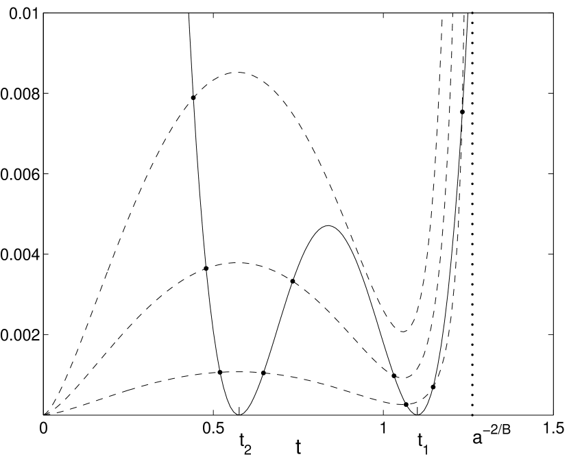
Figure 1: Graphs of $K_{2}(t)/(1-a^{2}t^{B})$ (dashed curves) and $-K_{1}(t)=(t-t_{1})^{2}(t-t_{2})^{2}$ (full curve) for the lens with $B=1.5$, $q=0.8$, $a=0.84$, $\gamma_{1}=0.1$, and $\gamma_{2}=0$. The intersections of the curves of different type correspond to images. The three dashed curves, from the lowest up, are for the three source positions $\zeta=|\zeta|\exp({4\pi i/9})$ for $|\zeta|=.08$, $|\zeta|=.15$, and $|\zeta|=.225$. These source positions give five, three, and one images respectively. Only for such a large core radius can a figure be drawn in which all the intersections and the asymptote $t=a^{-2/B}$ are visible on the same scale.

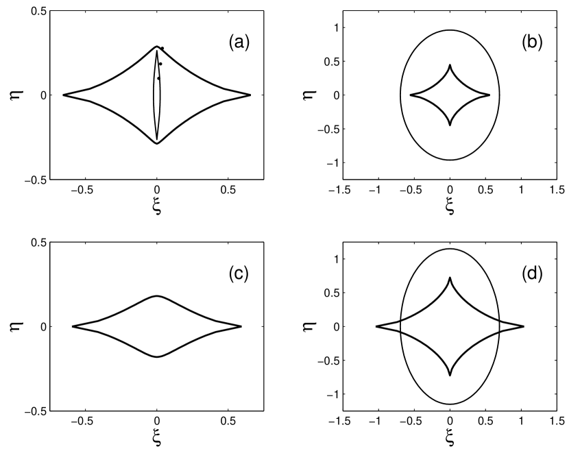
Figure 2: The four different caustic configurations which can occur with the cored elliptical potential (18). Case (a) is for the double lips caustic for the lensing potential of Fig. 1. The dots show the three different source positions, aligned and with increasing $|\zeta|$, for the dashed curves of Fig. 1. Case (b) is for the $B=2$, $q=0.8$, $a=0.1$, $\gamma_{1}=\gamma_{2}=0$ case for which Fig. 4 is plotted. The single lips case (c) differs from (a) only in having the larger core $a=1.0$ for which there is no radial caustic. Case (d) differs from (b) only in having the smaller axis ratio $q=0.7$. This model lies below the $B=2$ curve in Fig. 3 and has naked cusps.

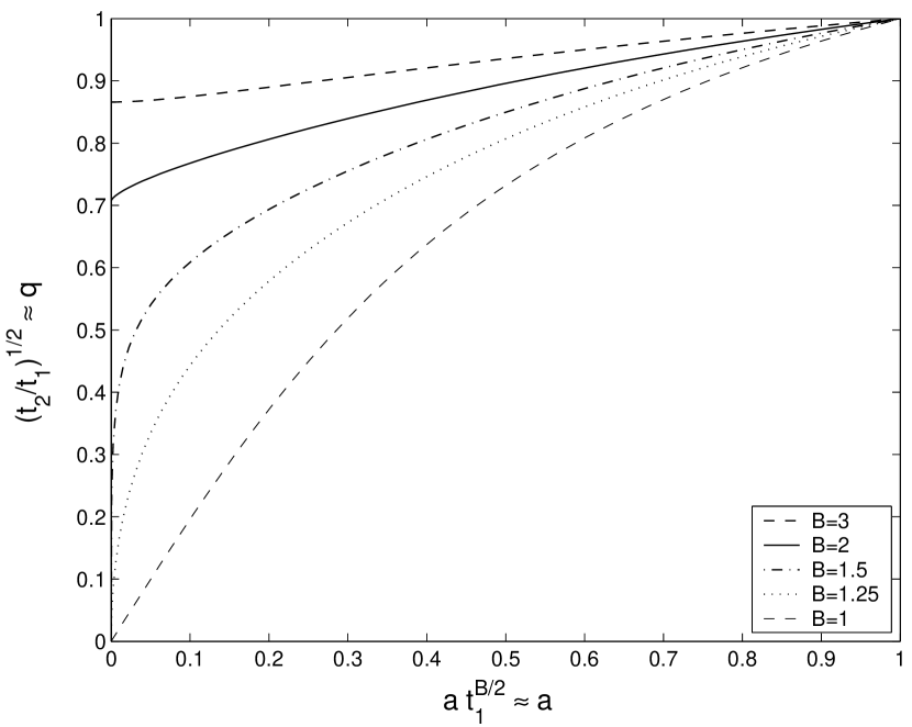
Figure 3: The regions of parameter space in which the tangential caustic has naked cusps are those which lie below the curves plotted. They grow as $B$ increases. The values of $t_{1}$ and $t_{2}$ depend on the shear. The approximations in the labels are those for negligible shear. The radial caustic balloons in size as $a\to 0$ for $B<2$, as predicted by equation (A7).

3.2 Magnifications of Pairs of Images

Changing the variable in the contour integral (14) for the magnification to $t$ gives

$$\sum_{{\rm images}}\mu_{i}p_{i}={q^{2}B\over 2\pi{\rm i}}\oint_{\cal C}{dt\over t}{P^{2}-|Q|^{2}\over(1-a^{2}t^{B})K}.$$ (25)

We write the denominator term as

$$(1-a^{2}t^{B})K={\hat{K}}_{1}+K_{2},$$ (26)

where we have labelled its two parts as

$${\hat{K}}_{1} = -(1-a^{2}t^{B})(P^{2}-|Q|^{2})^{2}=-(1-a^{2}t^{B})(t\!-\!t_{1})^{2}(t\!-\!t_{2})^{2},$$

$$K_{2} = t^{B}(P\zeta-Q{\bar{\zeta}})(P{\bar{\zeta}}-\bar{Q}\zeta).$$ (27)

The component $K_{2}$ is the same as in Paper I, whereas ${\hat{K}}_{1}$ differs from the $K_{1}=-(t-t_{1})^{2}(t-t_{2})^{2}$ of Paper I only through its extra $(1-a^{2}t^{B})$ factor, which is unity when there is no core.

In Paper I, we were interested primarily in sums over the four bright images. However, the contour integral (25), like the corresponding result in equation (23) of Paper I, applies equally well to any subset of the images provided that the contour ${\cal C}$ is chosen to enclose only the zeros of $(1-a^{2}t^{B})K$ which correspond to that subset. If $a<t_{2}^{-B/2}$ for instance, we define a contour ${\cal C}_{2}$ to be a simple closed contour in the complex $t$–plane which encircles the two direct images of even parity. These approach $t=t_{2}$ as $|\zeta|\to 0$, and so the contour ${\cal C}_{2}$ also encloses $t_{2}$ which lies in between, but it excludes all the other images, as well as $t=0$, $t=t_{1}$, $t=a^{-2/B}$ and any complex zeros of $(1-a^{2}t^{B})$. Then, we obtain the formula

$$\sum\limits_{{\hbox{\eightrm{2 direct}}}\atop{\hbox{\eightrm{images}}}}\mu_{i}p_{i}=\sum\limits_{{\hbox{\eightrm{2 direct}}}\atop{\hbox{\eightrm{images}}}}\mu_{i}={-q^{2}B\over 2\pi{\rm i}}\oint\nolimits_{{\cal C}_{2}}{dt\over t(t-t_{1})(t-t_{2})(1-a^{2}t^{B})\left(1+{K_{2}\over{\hat{K}}_{1}}\right)}.$$ (28)

We require that ${\cal C}_{2}$ keep a finite distance from $t_{1}$, $t_{2}$, and every zero of $(1-a^{2}t^{B})$. Then, with $|t|$ bounded above, and $|t-t_{1}|$, $|t-t_{2}|$, and $|1-a^{2}t^{B}|$ bounded from below, it follows that

$$\left|{K_{2}\over{\hat{K}}_{1}}\right| = \left|{t^{B}\over 1-a^{2}t^{B}}\right|\left|{|\lambda|^{2}\over(t-t_{1})^{2}}+{|\nu|^{2}\over(t-t_{2})^{2}}\right|$$ (29)

$$\leq \left|{t^{B}\over 1-a^{2}t^{B}}\right|\left[{|\lambda|^{2}\over|t-t_{1}|^{2}}+{|\nu|^{2}\over|t-t_{2}|^{2}}\right],$$

and hence $|{K_{2}/{\hat{K}}_{1}}|<1$ on ${\cal C}_{2}$ for sufficiently small $|\zeta|$. We have here used the result

$$(P\zeta-Q{\bar{\zeta}})(P{\bar{\zeta}}-\bar{Q}\zeta)=[\lambda(t_{2}-t)+\nu(t_{1}-t)][\bar{\lambda}(t_{2}-t)+\bar{\nu}(t_{1}-t)]=|\lambda|^{2}(t_{2}-t)^{2}+|\nu|^{2}(t_{1}-t)^{2},$$ (30)

where $\lambda$ and $\nu$ are the following two linear combinations of the complex source coordinates

$$\lambda={1\over 2}\left(\zeta+{Q{\bar{\zeta}}\over|Q|}\right),\qquad\nu={1\over 2}\left(\zeta-{Q{\bar{\zeta}}\over|Q|}\right),$$ (31)

which have the property $|\lambda|^{2}+|\nu|^{2}=|\zeta|^{2}$. With $|{K_{2}/{\hat{K}}_{1}}|<1$, we can now expand the $(1+K_{2}/{\hat{K}}_{1})^{-1}$ term in the integral (28) as a geometric series to get

$$\sum\limits_{{\hbox{\eightrm{2 direct}}}\atop{\hbox{\eightrm{images}}}}\mu_{i}p_{i} = {-q^{2}B\over 2\pi{\rm i}}\oint\nolimits_{{\cal C}_{2}}{dt\over t(t-t_{1})(t-t_{2})(1-a^{2}t^{B})}$$ (32)

$$-{q^{2}B\over 2\pi{\rm i}}\sum\limits^{\infty}_{j=1}\oint\nolimits_{{\cal C}_{2}}{t^{Bj-1}[|\lambda|^{2}(t-t_{2})^{2}+|\nu|^{2}(t-t_{1})^{2}]^{j}\over(t-t_{1})^{2j+1}(t-t_{2})^{2j+1}(1-a^{2}t^{B})^{j+1}}dt.$$

The restrictions that we imposed earlier on ${\cal C}_{2}$ guarantee that this series converges for sufficiently small $|\zeta|$. Every integral in it can be evaluated from its residue at $t=t_{2}$ alone because that is the only singularity within the contour ${\cal C}_{2}$. The leading order term is the residue of the simple pole at $t=t_{2}$, which is positive because both parities are even. The full expansion for the sum of the two magnifications is

$$\sum\limits_{{\hbox{\eightrm{2 direct}}}\atop{\hbox{\eightrm{images}}}}\mu_{i}={q^{2}B\over 2|Q|t_{2}(1-a^{2}t^{B}_{2})}+C_{2}(t_{1},t_{2},a^{2};\lambda,\nu).$$ (33)

Here, $C_{2}$ is a correction term which vanishes if the source is exactly aligned with the center of the lensing galaxy. More generally, it takes the form:

$$C_{2}(t_{1},t_{2},a^{2};\lambda,\nu)=q^{2}B\sum\limits^{\infty}_{j=1}\sum\limits^{j}_{m=0}{j\choose m}|\lambda|^{2m}|\nu|^{2j-2m}R_{2}(t_{1},t_{2},a^{2};j,2m,2j-2m),$$

where we have defined

$$R_{2}(t_{1},t_{2},a^{2};j,\ell,k)=-{1\over 2\pi{\rm i}}\oint\nolimits_{{\cal C}_{2}}{t^{Bj-1}dt\over(t-t_{1})^{\ell+1}(t-t_{2})^{k+1}(1-a^{2}t^{B})^{j+1}}.$$ (34)

In fact, we can obtain closed form expressions for all of these integrals without any further residue calculus by simple partial differentiation because

$$R_{2}(t_{1},t_{2},a^{2};j,\ell,k) = {1\over k!}{\partial^{k}\over\partial t^{k}_{2}}R_{2}(t_{1},t_{2},a^{2};j,\ell,0)$$

$$= -{1\over k!}{\partial^{k}\over\partial t^{k}_{2}}\left[{1\over(t_{2}-t_{1})^{\ell+1}}{t_{2}^{Bj-1}\over(1-a^{2}t^{B}_{2})^{j}}\right].$$

If the conditions for quintuple imaging are satisfied, then there is a pair of inverted images which approach $t=t_{1}$ as $|\zeta|\to 0$. We can perform a similar analysis for a simple closed contour ${\cal C}_{1}$ in the complex $t$-plane which encloses the images and $t_{1}$, but not $t=0$, $t=t_{2}$, $t=a^{-2/B}$ or any complex zero of $(1-a^{2}t^{B})$. The result is that

$$\sum\limits_{{\hbox{\eightrm{2 inverted}}}\atop{\hbox{\eightrm{images}}}}\mu_{i}p_{i}=-\sum\limits_{{\hbox{\eightrm{2 inverted}}}\atop{\hbox{\eightrm{images}}}}\mu_{i}={-q^{2}B\over 2|Q|t_{1}(1-a^{2}t^{B}_{1})}+C_{1}(t_{1},t_{2},a^{2};\lambda,\nu),$$ (36)

where the correction term $C_{1}$ is

$$C_{1}(t_{1},t_{2},a^{2};\lambda,\nu)=q^{2}B\sum\limits^{\infty}_{j=1}\sum\limits^{j}_{m=0}{j\choose m}|\lambda|^{2m}|\nu|^{2j-2m}R_{1}(t_{1},t_{2},a^{2};j,2m,2j-2m).$$ (37)

Here, we have defined

$$R_{1}(t_{1},t_{2},a^{2};j,\ell,k) = -{1\over 2\pi i}\oint\nolimits_{{\cal C}_{1}}{t^{Bj-1}dt\over(t-t_{1})^{\ell+1}(t-t_{2})^{k+1}(1-a^{2}t^{B})^{j+1}}$$

$$= {1\over\ell!}{\partial^{\ell}\over\partial t^{\ell}_{1}}R_{1}(t_{1},t_{2},a^{2};j,0,k)$$

$$= -{1\over\ell!}{\partial^{\ell}\over\partial t^{\ell}_{1}}\left[{1\over(t_{1}-t_{2})^{k+1}}{t^{Bj-1}_{1}\over(1-a^{2}t^{B}_{1})^{j}}\right]$$

$$= R_{2}(t_{2},t_{1},a^{2};j,k,\ell).$$

In fact, the coefficients $R_{1}(t_{1},t_{2},a^{2};j,\ell,k)$ and $R_{2}(t_{1},t_{2},a^{2};j,\ell,k)$ can be expressed as finite sums, as is demonstrated in Appendix B.

Neither series (33) nor (36) remains convergent at the tangential caustic where one of the direct and one of the inverted images merge; the magnifications of the merging images become infinite and one cannot then construct the ${\cal C}_{1}$ and ${\cal C}_{2}$ contours. However, the sum of series (33) and (36) can remain convergent at the tangential caustic because the infinities of the signed magnifications of the two merging images cancel. The series (36) ceases to converge at the radial caustic where an inverted and a doubly inverted image merge, but the series (33) for the direct images converges there if, as in Fig. 2a, it lies inside the tangential caustic.

Let us note some interesting special cases of the preceding formulae. In the scale-free limit ($a=0$) when $B=1$ or $B=2$, then remarkably the correction terms have the property that $C_{1}-C_{2}\equiv 0$. As first discovered by Witt & Mao (2000; see also Paper I), the sum of the four signed magnifications is then an invariant completely independent of the source position

$$\sum\limits_{{\hbox{\eightrm{4 images}}}}\mu_{i}p_{i}=\frac{B}{1-\gamma_{1}^{2}-\gamma_{2}^{2}}.$$ (39)

Even though this result is not exact for other values of $B$, it is often an extremely good approximation. If the core radius is non-zero, then the sum of the signed magnifications becomes

$$\sum\limits_{{\hbox{\eightrm{4 images}}}}\mu_{i}p_{i}\approx\frac{B}{(1-\gamma_{1}^{2}-\gamma_{2}^{2})(1-a^{2}t_{1}^{B})(1-a^{2}t_{2}^{B})}\left[1-{a^{2}(t_{1}^{B+1}-t_{2}^{B+1})\over t_{1}-t_{2}}\right],$$ (40)

and this approximation remains remarkably accurate inside the radial caustic. An example is the cored isothermal lens of Fig. 2b. The sum of the four signed magnifications is constant to within tenths of one percent over all of the region inside the tangential caustic except very close to the cusps. However, the smallness of the dependence of that sum on the source position is due to a near-cancellation of the correction terms in the two image sums. Fig. 4 shows how much the sum of the magnifications of the two direct images varies over the same region. Numerically, the leading coefficients in expansion (3.2) for $C_{2}$ are $R_{2}(t_{1},t_{2},a^{2};1,2,0)=13.77$ and $R_{2}(t_{1},t_{2},a^{2};1,0,2)=21.64$. The sums $R_{1}+R_{2}$ for the same sets of indices are -0.01. Though numerical values vary, $R_{1}+R_{2}$ is typically at least two orders of magnitude less than $R_{2}$ for lenses with small cores and with an inner tangential caustic. In Section B.3, we show how near-cancellation can occur more generally from the contour integral formula (14), and is not a peculiarity of power-law galaxies. However, this behavior is not universal. The sum of the four signed magnifications has large variations over the region inside the inner radial caustic of Fig. 2a, while the sum of the magnifications of the two direct images changes little in the middle third of that region. That middle third lies well inside the tangential caustic at which the direct image sum becomes large.

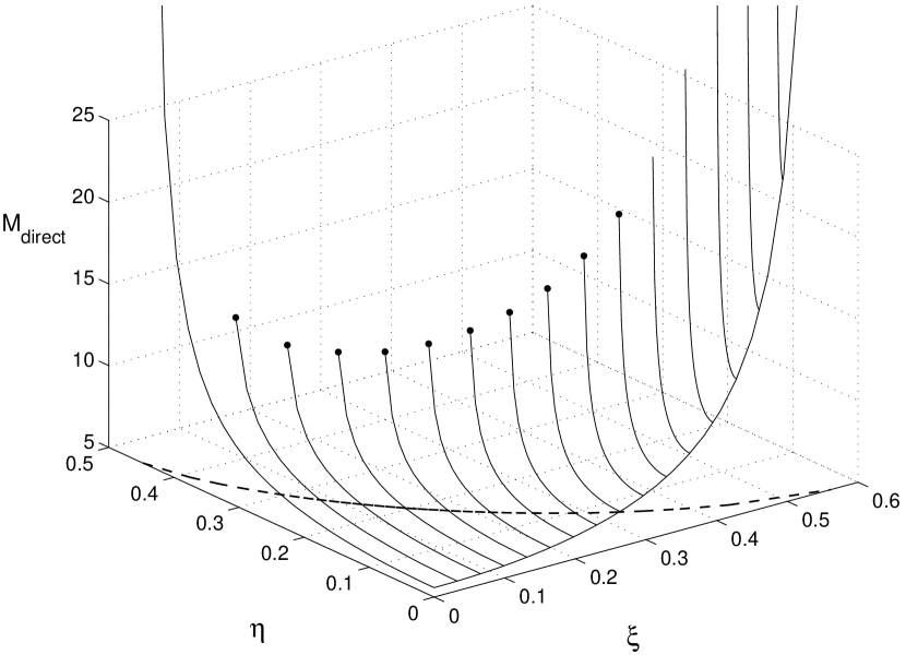
Figure 4: The surface given by the sum of the magnifications of the two direct images for $B=2$, $q=0.8$, $a=0.1$, $\gamma_{1}=\gamma_{2}=0$ over the first quadrant of the $(\xi,\eta)$-plane inside the tangential caustic. That caustic is drawn as the dashed curve on the base of the plot. The full curves are the intersection of the surface with the planes $\eta=0$, and evenly spaced planes $\xi={\rm const}$. The filled circles denote the points at which $\eta$ is $0.96$ of its value at the caustic. Curves which do not end with filled circles exceed 25 before getting that close to the caustic.

The separate sums of the pairs contain more information than their signed combination. Physically speaking, it is the total magnification (that is, the sum of the magnifications) which is more interesting, but this varies considerably with source position. The minimum magnification $A_{\rm min}$ in the scale-free limit $(a=0)$ is

$$A_{\rm min}=\sum\limits_{{\hbox{\eightrm{4 images}}}}\mu_{i}={B\over 1-\gamma_{1}^{2}-\gamma_{2}^{2}}{P_{0}\over|Q|}$$ (41)

This corresponds to the case when the source is aligned with the center of the lensing galaxy. It is a good approximation only when the source offset is small. For non-zero core radius, it becomes

$$A_{\rm min}=\sum\limits_{{\hbox{\eightrm{4 images}}}}\mu_{i}={B\over 1-\gamma_{1}^{2}-\gamma_{2}^{2}}{1\over 2|Q|}\left[{t_{2}\over 1-a^{2}t_{1}^{B}}+{t_{1}\over 1-a^{2}t_{2}^{B}}\right].$$ (42)

In the next section, we discuss another nearly constant four-image sum which reduces to the sum of the unsigned magnifications when the source is aligned with the center of the lensing galaxy.

3.3 Configuration Moments

The contour integral method can also be used to calculate configuration moments, that is, sums over the images of products of the signed magnifications with position coordinates. Those sums are obtained by adding the complex position coordinates from (7) to the sum (14) to obtain

$$\sum_{{\rm images}}\mu_{i}p_{i}z_{i}^{m}{\bar{z}}_{i}^{n}={-q^{2}\over 2\pi{\rm i}}\oint_{\cal C}{d\tau\over\tau}{(P\zeta-Q{\bar{\zeta}})^{m}(P{\bar{\zeta}}-{\bar{Q}}\zeta)^{n}\over K(\tau;\zeta,{\bar{\zeta}})(P^{2}-|Q|^{2})^{m+n-1}}.$$ (43)

We expand for moments in the same manner as for the magnifications, with the result that

$$\sum\limits_{{\hbox{\eightrm{2 direct}}}\atop{\hbox{\eightrm{images}}}}\mu_{i}z^{m}_{i}\mathop{\bar{z}}\nolimits^{n}_{i}={-qB^{2}\over 2\pi i}\sum\limits^{\infty}_{j=0}\oint\nolimits_{{\cal C}_{2}}{t^{Bj-1}[\lambda(t_{2}-t)+\nu(t_{1}-t)]^{m+j}[\mathop{\bar{\lambda}}\nolimits(t_{2}-t)+\mathop{\bar{\nu}}\nolimits(t_{1}-t)]^{n+j}dt\over[(t-t_{1})(t-t_{2})]^{2j+m+n+1}(1-a^{2}t^{B})^{j+1}}.$$ (44)

After the two numerator factors are expanded binomially, we see that every integral is of the same form as (34), and so, provided $m+j\geq 0$ and $n+j\geq 0$, we obtain

$$\sum\limits_{{\hbox{\eightrm{2 direct}}}\atop{\hbox{\eightrm{images}}}}\!\!\!\!\!\! \mu_{i}z^{m}_{i}\mathop{\bar{z}}\nolimits^{n}_{i}=(-1)^{m+n}q^{2}B\sum\limits^{\infty}_{j=0}\sum\limits^{2j+m+n}_{\ell=0}R_{2}(t_{1},t_{2},a^{2};j,\ell,2j+m+n-\ell)$$ (45)

$$\times\sum\limits^{\min(\ell,m+j)}_{k=\max(0,\ell-n-j)}{m+j\choose k}{n+j\choose\ell-k}\lambda^{k}\mathop{\bar{\lambda}}\nolimits^{\ell-k}\nu^{m+j-k}\mathop{\bar{\nu}}\nolimits^{n+j+k-\ell}.$$

The corresponding sum for the indirect pair is

$$\sum\limits_{{\hbox{\eightrm{2 inverted}}}\atop{\hbox{\eightrm{images}}}}\!\!\!\!\!\! \mu_{i}z^{m}_{i}\mathop{\bar{z}}\nolimits^{n}_{i}=(-1)^{m+n+1}q^{2}B\sum\limits^{\infty}_{j=0}\sum\limits^{2j+m+n}_{\ell=0}R_{1}(t_{1},t_{2},a^{2};j,\ell,2j+m+n-\ell)$$ (46)

$$\times\sum\limits^{\min(\ell,m+j)}_{k=\max(0,\ell-n-j)}{m+j\choose k}{n+j\choose\ell-k}\lambda^{k}\mathop{\bar{\lambda}}\nolimits^{\ell-k}\nu^{m+j-k}\mathop{\bar{\nu}}\nolimits^{n+j+k-\ell}.$$

In either case the same $R_{1}$ and $R_{2}$ functions as arise with the magnifications, and which are evaluated in Appendix B, are all that is needed.

Whereas the present paper is mostly concerned with magnifications, our modeling in Paper I made use of configuration moments too. The analysis of this paper, and especially that of Appendix Section B.3, shows that four-image sums of moments may also be far more uniform than the separate sums (45) and (46) because of cancellations. However it is possible to mitigate the cancellations which arise from signed magnifications by using specially contrived configuration moments. As an example, consider the zeroth order $m=1$, $n=-1$ moment [see eqn. (48) of Paper I] in which the magnifications are weighted by the complex exponential $e^{2i\Phi}$, where $z=|z|e^{i\Phi}$. The angle $\Phi$ for each image is $\arctan(y_{i}/qx_{i})$This factor exactly compensates for the different signs of the magnifications when the source offset is zero and the two kinds of images lie on perpendicular lines through $O$. We obtain the $j=0$ terms directly from the integral (44) and its pair because the binomial expansions used to obtain equations (46) and (45) are not valid when $n+j<0$. This gives us two $R(t_{1},t_{2},a^{2};0,0,0)$ integrals whose sum gives

$$\sum\limits_{{\hbox{\eightrm{4 images}}}}\mu_{i}p_{i}e^{2i\Phi_{i}}\approx{-B\over(1-\gamma_{1}^{2}-\gamma_{2}^{2})}{1\over 2{\bar{Q}}}\left[{t_{2}\over 1-a^{2}t_{1}^{B}}+{t_{1}\over 1-a^{2}t_{2}^{B}}\right],$$ (47)

because $\lambda/\mathop{\bar{\lambda}}\nolimits=-\nu/\mathop{\bar{\nu}}\nolimits=Q/|Q|$. The sum (47) is minus the sum in equation (42) when there is no off-axis shear and $Q$ is real because $e^{2i\Phi}=1$ on the major $x$-axis where the inverted images initially lie and $e^{2i\Phi}=-1$ on the minor $y$-axis. Off-axis shear rotates the configuration and $\bar{Q}/|Q|$ is then the complex factor which makes $\sum\limits_{{\hbox{\eightrm{4 images}}}}\mu_{i}p_{i}(\bar{Q}e^{2i\Phi}/|Q|)$ real. This four-image sum can remain nearly constant as the source offset changes because the changing angular positions of the images counteracts their changing magnitudes. For the cored isothermal lens for which Fig. 2b and Fig. 4 are plotted for example, the $m=1$, $n=-1$ moment of equation (47) displays the same near constancy over the region inside the tangential caustic as does the sum of the four signed magnifications. Estimates of $q$ and the orientation of the lens must be combined with observed positions to evaluate the sum in (47), but the result should be real when multiplied by $\bar{Q}/|Q|$.

3.4 The Magnification of the Central Image

There is no fifth central image in the absence of a core for $B\leq 2$. When there is a core, the central image is given by the root of the imaging equation (26) for which $t\to a^{-2/B}$ and $\tau\to 0$ as $|\zeta|\to 0$. We can obtain formulae for its signed magnification involving another set of $R$-functions, defined by

$$R_{a}(t_{1},t_{2},a^{2};j,\ell,k)={-1\over 2\pi i}\oint\nolimits_{{\cal C}_{a}}{t^{Bj-1}dt\over(t-t_{1})^{\ell+1}(t-t_{2})^{k+1}(1-a^{2}t^{B})^{j+1}}$$ (48)

where ${\cal C}_{a}$ is a loop enclosing $t=a^{-2/B}$ but not $t_{1}$ or $t_{2}$ or $0$ or any other zeros of $(1-a^{2}t^{B})$. These functions can be calculated by evaluating residues at $t=a^{-2/B}$. This is a simple pole when $j=0$, and we then get

$$R_{a}(t_{1},t_{2},a^{2};0,\ell,k)={a^{2(\ell+k+2)/B}\over B[1-a^{2/B}t_{1}]^{\ell+1}[1-a^{2/B}t_{2}]^{k+1}}.$$ (49)

The signed magnification of the central image is given by

$$\mu_{a}p={q^{2}a^{4/B}\over[1-a^{2/B}t_{1}][1-a^{2/B}t_{2}]}+C_{a}(t_{1},t_{2},a^{2};\lambda,\nu).$$ (50)

where the correction term $C_{a}(t_{1},t_{2},a^{2};\lambda,\nu)$ has the form

$$C_{a}(t_{1},t_{2},a^{2};\lambda,\nu)=q^{2}B\sum\limits^{\infty}_{j=1}\sum\limits^{j}_{m=0}{j\choose m}|\lambda|^{2m}|\nu|^{2j-2m}R_{a}(t_{1},t_{2},a^{2};j,2m,2j-2m).$$ (51)

The lowest order term in (50) is positive if $a^{-2/B}>t_{1}$ when this image is doubly inverted, negative if $t_{1}>a^{-2/B}>t_{2}$ and the image is simply inverted, and positive if $t_{2}>a^{-2/B}$ and it is the only and direct image.

When $a$ is small, as in our applications, so that $a^{-2/B}\gg t_{1}$ and the central image occurs for a large value of $t$, equations (50) and (51) can be approximated by

$$\mu_{a}p=\mu_{a}=q^{2}a^{4/B}+q^{2}B\sum\limits^{\infty}_{j=1}|\zeta|^{2j}R_{a}(0,0,a^{2};j,2j,0).$$ (52)

These special cases of integrals (48) can be evaluated by residues (change to $a^{2}t^{B}-1$ as integration variable) and give a series expansion for the magnification of the central image as

$$\mu_{a}=q^{2}a^{4/B}\left[1+\sum\limits^{\infty}_{j=1}\alpha_{j}(|\zeta|^{2}a^{2(2-B)/B})^{j}\right],\quad\alpha_{j}={\Gamma\left[{2(j+1)\over B}+1\right]\over j!\Gamma\left[{2(j+1)\over B}+1-j\right]}.$$ (53)

The series is especially simple for $B=2$ when it is binomial and gives

$$\mu_{a}={q^{2}a^{2}\over(1-|\zeta|^{2})^{2}}.$$ (54)

There are also two cases for which the series is hypergeometric and can be summed explicitly. They are $B=1$, for which

$$\mu_{a}={4q^{2}a^{4}\over\sqrt{1-4|\zeta|^{2}a^{2}}[1+\sqrt{1-4|\zeta|^{2}a^{2}}]^{2}},$$ (55)

and $B=4$, for which

$$\mu_{a}=q^{2}a\left[{|\zeta|^{2}\over a}+{1+|\zeta|^{4}/2a^{2}\over\sqrt{1+|\zeta|^{4}/4a^{2}}}\right].$$ (56)

The reason for the simplifications is that they are most easily obtained directly from the basic magnification formula (25) after its integrand is approximated for large $t$ to give

$$\mu_{a}={q^{2}B\over 2\pi i}\oint\nolimits_{{\cal C}_{a}}{dt\over t^{3}[t^{B-2}|\zeta|^{2}-1+a^{2}t^{B}]}.$$ (57)

The root for the central image and its residue can be calculated directly without any need for series expansion for the three special values of $B$. More generally, series expansion is needed. This analysis makes it clear that the basic requirement for the approximation (53) to be valid is that $t$ be large at the central image.

It is evident that the series (53) shows $\mu_{a}$ to be an increasing function of $|\zeta|^{2}a^{2(2-B)/B}$ for $B\leq 2$ because all its coefficients $\alpha_{j}$ are then positive. Numerical evaluation, as in Fig. 5, shows that $\mu_{a}$ remains an increasing function for larger $B$. Those plots extend to $96\%$ of the radius of convergence. The series converge for

$$|\zeta|^{2}<\left({B\over 2}\right)a^{2(B-2)/B}\left|{B\over 2}-1\right|^{(2-B)/B},$$ (58)

as follows from using Stirling’s formula to approximate the gamma functions and standard convergence tests. Hence the range of usefulness of the series depends considerably on the value of $B$. For $B\leq 2$ and $a$ small, the radius of convergence is large, and the series converges out to the radial caustic as approximated by equation (A7). The magnification of course becomes large as the caustic, at $|\zeta|=1$ for $B=2$ and $|\zeta|=1/2a$ for $B=1$, is approached. For $B>2$ on the other hand, the radius of convergence is caused by the breakdown of the approximation that the central image occurs for large $t$ and, as with equation (56), $\mu_{a}$ remains finite as the condition (58) is violated. That radius of convergence in $|\zeta|$ is proportional to the positive power $a^{1-2/B}$. Consequently, the approximation (53) is useful for only a small part of the region within the radial caustic when the core radius $a$ is small, and $\mu_{a}$, which is growing with source offset on a short length-scale, can continue to become considerably larger before the radial caustic is approached.

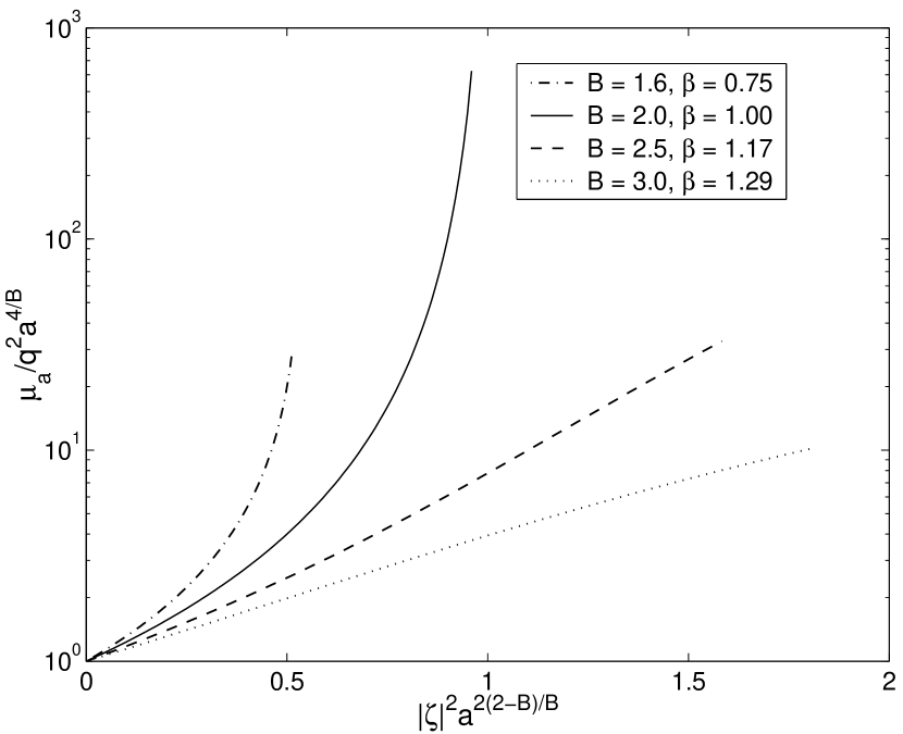
Figure 5: Sums of the series (53) for the scaled magnification of the central image as functions of its scaled argument out to $96\%$ of their radii of convergence. Those radii vary with $B$ as in equation (58). The location of the radius of convergence approximates the radial caustic for the top two curves with $B\leq 2$. The near-linear growth with increasing source offset of the lower two curves for $B>2$ is a little less than, but growing towards, the $B>2$ estimate $|\zeta|^{4/(B-2)}$ of equation (51) of Paper I.

Numerical tests shows that the approximation (53) works well where the theory predicts that it will; over much of the region within the radial caustic for $B\leq 2$, but only in limited central regions for $B>2$. It underestimates $\mu_{a}$ because of the neglect of denominator terms such as those at the leading order in equation (50). That underestimate can be by 10 % or more for $a=0.1$, but accuracy increases substantially for smaller $a$.

Figure 6: The percentage of quintuplets with a visible central image is plotted against the slope of the surface density. If the model is nearly singular, then $2/B>1$ for cusps steeper than isothermal, while $2/B<1$ for cusps shallower than isothermal. The four panels show results for different values of the core radius $a$. There is no fifth image when $a=0$ and $2/B\geq 1$. In each panel, the full line denotes $q=0.7$, the dotted line $q=0.8$ and the dashed line $q=0.9$ models. The threshold is $1\%$.

Figure 7: The percentage of core triplets with a visible central image is plotted against the slope of the surface density. The four panels show results for different values of the core radius $a$. In each panel, the full line denotes $q=0.7$, the dotted line $q=0.8$ and the dashed line $q=0.9$ models. The threshold is $1\%$.

Figure 8: The percentage of naked cusp triplets with a visible central image is plotted against the slope of the surface density. The two panels show results for different values of the core radius $a$. In each panel, the full line denotes $q=0.7$, the dotted line $q=0.8$ and the dashed line $q=0.9$ models. The threshold is $1\%$.

4 Application: The Missing Central Images

Here, we study the problem of missing central images from the standpoint of the structure of the lensing galaxy. In optical lenses, the experimental constraint is weak, as any central image can be masked by emission from the lensing galaxy. Radio-loud lenses provide much stronger constraints, as they have typically been probed with high dynamic range radio maps. The Cosmic Lens All-Sky Survey (CLASS) is the largest statistically homogeneous search for gravitational lenses (e.g., Myers 1999). The survey sample contains $\sim 10^{4}$ flat-spectrum radio sources. In the best cases, such as B0218+357 (Biggs et al. 1999) and B1030+074 (Xanthopoulos et al. 1998), the magnification ratio of the faintest to the brightest image $r$ is constrained to $\mathrel{\hbox to0.0pt{\lower 3.0pt\hbox{$\sim$}\hss}\raise 2.0pt\hbox{$<$}}0.1\%$ from the absence of a detectable central image in the map. As a typical detection limit in the below calculations, we adopt $r\approx 1\%$ for central images. This is appropriate for radio lenses, but not for optical lenses.

We perform Monte Carlo simulations using the power-law galaxies (18). Sources are placed randomly within the outermost caustic for choices of $\beta$, $q$ and core radius $a$. The imaging equation (22) is solved numerically to find the roots $t$ of the images. We then evaluate the magnifications using (13), and work out the ratio of the brightest to the faintest image. Repeating this many times gives us the raw probabilities of observing a central image.

Figs 6-8 show the probability of observing a central image as a function of the slope of the projected density ($2/B=2-\beta$) for the case of the quintuplets, the core triplets and the naked cusp triplets respectively. The panels show how the raw probabilities depend on the core radius $a$, while the different lines in each panel show different flattenings. The models have a singular density profile if $a=0$, and are very nearly singular when $a$ is small. We describe the parameter $2/B$ as the slope index, as it controls the fall-off of the projected density. For the isothermal cusp, $2/B=1$ and so the projected density $\kappa\sim{\rm distance}^{-1}$. Models steeper than isothermal have $2/B>1$, models shallower than isothermal have $2/B<1$.

There are a number of things to notice in Fig. 6. As the core radius $a$ is diminished, the régime in which the central image is visible shrinks. Visible central images occur only for $B>2$ when the central image is stronger as the simple estimate $\mu_{a}\approx q^{2}a^{4/B}$ from §3.4 predicts. The full curves for the flattened ($q=.7$) models lie above the dashed curves for the rounder ($q=.9$) models. This is due to a stronger dimming of the brightest image with increasing flattening which outpaces the dimming of the central image. All magnifications share a $q^{2}$-dependence which comes from the basic magnification formula (25). The brightest image is direct for vanishing shear and zero source offset, and has magnification $\mu_{1}\approx q^{2}B/(4|Q|t_{2})=B/2(1-q^{2})$. Hence we estimate the ratio of the central image to the brightest image at zero source offset to be $\mu_{a}/\mu_{1}\approx 2q^{2}(1-q^{2})Ba^{4/B}$. This ratio increases with increasing flattening. For small $a$, the magnification of the central image does not vary greatly with increasing source offset within the quintuplet region for $B\leq 2$. This region inside the tangential caustic is but a small part of that within the radial caustic, and hence the abscissa of Fig. 5 varies little. Conversely, the brightest image strengthens considerably with increasing source offset as it gets closer to the tangential caustic. The result is that the ratio $\mu_{a}/\mu_{1}$ of central to brightest magnifications decreases with increasing source offset for $B\leq 2$. For $B>2$ on the other hand, $\mu_{a}$ grows so strongly across the quintuplet region that it can outpace the growth of $\mu_{1}$. The net result is that the flatter the potential, and the larger the core radius, then the greater is the likelihood that the central image is bright enough to be visible.

Fig. 7 shows the raw probability of observing a central image for core triplets. The behavior of the curves as a function of slope index $2/B$ has the following explanation. If $2/B$ is too large, then the central image is highly demagnified and so the raw probability is vanishingly small. As the slope index $2/B$ diminishes, the central image becomes brighter and the probability rises quickly to $100\%$. The brightest image is generally the remaining direct one. It dims with increasing source offset whereas the central image brightens. The tangential caustic also grows in size as $q$ decreases for constant slope index. That is the main reason why central images are more visible with increased flattening for $B>2$; the average source offset in the core triplet region between the tangential and radial caustics is then larger, and hence $\mu_{a}$ is significantly larger. As $2/B$ decreases further, the astroidal tangential caustic grows, and the area in the source plane generating core triplets diminishes and eventually vanishes, as the tangential caustic becomes larger than the radial caustic as in Fig. 2c. The smaller $q$ is, the sooner this happens and, as Fig. 7 shows, the size of the core has little effect on the stage at which the core triplet region disappears. The second and third terms of the inequality (24) become equal at that stage and, in the absence of shear, $2/B$ is then $(1-q^{2})/(1-a^{2})$ (See Appendix A). If the core radius $a\mathrel{\hbox to0.0pt{\lower 3.0pt\hbox{$\sim$}\hss}\raise 2.0pt\hbox{$>$}}0.01$, then even models steeper than isothermal ($\beta<1$) can provide observable central images. For smaller core radii ($a<.01$), the visible central images are confined to models less steep than isothermal. Notice that the constraints on the maximum possible steepness of the lensing potential provided by the missing image are stronger for doublets than quadruplets once $a\mathrel{\hbox to0.0pt{\lower 3.0pt\hbox{$\sim$}\hss}\raise 2.0pt\hbox{$<$}}.01$. For small core radii, the fifth image in quintuplet systems is significantly more demagnified than the third image in triplet systems. However, for larger core radii, it is the quadruplets that provide the stronger restriction.

Fig. 8 shows the raw probability of observing a central image for naked cusp triplets. Naked cusps are much less abundant for elliptic potentials as opposed to elliptic densities (Kassiola & Kovner 1993). Almost as soon as naked cusps appear, all three images are of roughly similar brightness and they are all detectable. Hence, the raw probability of observing a central image shows a swift transition from nearly $0\%$ to nearly $100\%$ as soon as naked cups become possible. The Monte Carlo results are consistent with the transitions given in Fig. 3. Equations (A) predict that the transitions occur at the values $2/B=0.565,\;0.913,\;1.157,$ for $a=0.1$ and $2/B=0.542,\;0.850,\;1.004,$ for $a=10^{-5}$. There are no strong observational candidates for naked cusp triplets, and so we must conclude that Fig. 8 sets a firm lower limit on the slope index $2/B$. This must be larger than the critical value which permits naked cusps (given in Fig. 3), otherwise naked cusps would be common.

To compare with data from surveys, we must allow for the amplification bias. Lens systems with a high total magnification $\mu$ are preferentially included in a flux-limited survey (e.g., Turner 1980, Turner, Ostriker & Gott 1984). The flux distribution of the sources in CLASS is well described by $dN/dS\propto S^{-2.1}$, where $N$ is the number of sources with flux greater than $S$ (Rusin & Tegmark 2001). For a flux limited sample, the probabilities that take into account amplification bias are

$$P=\int_{\cal A}d\xi d\eta\left[\mu(\xi,\eta)\right]^{1.1}$$ (59)

where ${\cal A}$ denotes the area enclosed by the caustics in the source plane for which the central image passes the threshold (e.g., Rusin & Ma 2001). Fig. 9 is the analogue of Fig. 7 when amplification bias is taken into account. Only the rightmost branch of the curve is plotted, as this is the most relevant for constraining the core size and the slope index. Notice that the effects of the amplification bias cause only slight changes in the shapes of the curves. Once the core radius falls below $a\approx 0.01$, then irrespective of the flattening, the lensing potential is constrained to be at least as steep as isothermal to ensure that the fraction of triplets with an observable central image remains low. As Fig. 10 shows, this conclusion remains valid even in the presence of shear. Shear has little direct effect on the magnitude of the central image as equation (53), which is independent of shear, predicts. However, shears of the order of 0.1 cause the inner tangential caustic to grow significantly in size for the $2/B$ values at which the curves of Fig. 10 rise sharply, while the radial caustic merely tilts a little. The greater visibility of the central image is again because the average source offset in the diminished core triplet region has become larger, now as a result of shear. The total shear produced by internal misalignments, large-scale structure and neighboring galaxies is typically constrained by $|\gamma|\mathrel{\hbox to0.0pt{\lower 3.0pt\hbox{$\sim$}\hss}\raise 2.0pt\hbox{$<$}}0.3$.

Figure 9: The percentage of triplets with a visible central image is plotted against the slope of the surface density. This figure incorporates the amplification bias, i.e., the tendency of high magnification configurations to be preferentially included in a flux-limited sample. The threshold is $1\%$. The increase of visibility with increasing flattening is now due primarily to the increasing size of the inner tangential caustic, which subtracts an area of weaker central images from the triplet region.

Figure 10: This figure shows the effects of external shear. For models with $a=0.01$, $q=0.8$, the percentage of triplets with a visible central image is shown for a range of values of the shear components. The threshold is $1\%$.

Figure 11: The percentage of triplets with a visible central image is plotted against the threshold (expressed as a percentage). The effects of amplification bias are included. The four panels show results for different slope indices ($0.75,1.0,1.25$ and $1.5$). In each panel, the full line denotes $q=0.7$, the dotted line $q=0.8$ and the dashed line $q=0.9$ models. The core radius $a=0.01$.

What restriction is implied on the core radius $a$ from the data on radio lenses? The CLASS survey found no triples, but 7 doublets. There is perhaps only 1 definite triple system (APM08279+5255) out of a total of $\sim 50$ doublets and triplets on Pospieszalka et al.’s gravitational lensing database (which contains both radio and optical lenses). So, the probability of detecting a triple with an observable central image is certainly very low. In this paper, we take it to be $\mathrel{\hbox to0.0pt{\lower 3.0pt\hbox{$\sim$}\hss}\raise 2.0pt\hbox{$<$}}2\%$ for radio lenses (i.e., at the $1\%$ threshold). Using Fig. 9, the top left panel showing curves for $a=0.1$ suggests that detectable central images are common for isothermal (or nearly so) galaxies. The smallest core radius $a$ seemingly compatible with the missing central images is $a\approx 0.01$ if the galaxy is isothermal. At a typical lens redshift of $z_{\rm l}\approx 0.5$ and a typical source redshift $z_{\rm s}\approx 2.5$, this corresponds to a physical size of $\approx 50$ pc (using formula (11) of Young et al. (1980) and formula (2.4) of Wallington & Narayan (1993)). The result holds good for a flat, matter-dominated Friedman-Robertson-Walker universe with a Hubble constant $H_{0}=75\,{\rm kms}^{-1}{\rm Mpc}^{-1}$. Suppose instead we use the currently popular cosmological model in which $\sim 70\%$ of the mean energy density required to make space flat is in the form of material for which gravity acts repulsively and the remaining $\sim 30\%$ is carried by collisionless massive particles of some type. Then the physical size of the core radii of isothermal galaxies is $\approx 70$ pc. These results are good for $2/B=1$. From the top right panel of Fig. 9, the dimensionless core radius can be increased to $a\approx 0.05$ if the galaxy has a larger slope index (say $2/B\approx 1.3$, which we will argue shortly is appropriate for giant ellipticals). In the same two cosmological models and with the same assumptions as to typical source and lens redshifts, this gives physical sizes of the core radius of $\approx 260$ pc and $\approx 350$ pc respectively, consistent with almost all the central images being absent.

Most of the optical depth to strong lensing resides in giant elliptical galaxies. Faber et al. (1997) analyse Hubble Space Telescope surface photometry of nearby ellipticals. They provide convincing evidence that giant elliptical galaxies have cuspy cores with steep outer power-law profiles and shallow inner profiles separated by a break radius. This is in contrast to low luminosity ellipticals, which have power-law surface brightness profiles. There are 26 giant ellipticals with cuspy cores presented in Table 2 of Faber et al. The mean value of the asymptotic outer slope of the surface brightness is $1.28$ with a standard deviation of $0.21$. This corresponds to the slope index or $2/B$ in the notation of this paper. The mean break radius is $330$ pc, which corresponds to only a few tens of millarcseconds at a typical lens redshift of $z_{\rm l}\approx 0.5$. The bright images of strong lenses are therefore probing the steep outer part of the cuspy core profile. The light profile is much steeper than isothermal; however, the projected mass may be less steep depending on the distribution of dark matter. Central images are absent because break radii are small in cuspy core galaxies and so the steep slope continues to small radii. In fact, only 2 out of the 26 galaxies listed by Faber et al. (1997) have a sufficiently shallow profile for the central image to stand any chance of being visible at the $1\%$ threshold. This provides an explanation of why most central images are unobservable at the current thresholds.

Other than a central black hole, there is little evidence for dark matter inside the inner 10 kpc of early-type galaxies that cannot be simply assigned to the stellar mass (e.g., Gerhard et al. 2001). Beyond 10 kpc or so, there probably is dark matter, although there are few hard facts on its distribution in ellipticals because of the absence of tracers at large radii. The dynamical evidence refers to the mass within spheres, whereas lensing is concerned with the mass within cylinders. Dark matter at large radii may alter the slope of the projected mass distribution in the inner few kpc. However, provided the slope remains isothermal or steeper and the break radius remains small, then the central image remains unobservable.

Fig. 11 shows the percentage of triplets with a visible central image as a function of the threshold for four different slope indices. Notice that for models with slopes steeper than isothermal, flattening typically makes the central image less visible, the reverse of the case when the slope is weak. The latter case shows the same trends as in the $a=0.01$ panel of Fig. 7. The radial caustic is large when $B<2$ and the tangential caustic occupies a much smaller part of the space within it. Both $\mu_{a}$ and $\mu_{1}$ now decrease as $q$ decreases, but $\mu_{a}$ decreases faster to make the central image less visible. Fig. 11 shows us that the fraction of detectable images is a strong function of the threshold. It enables us to predict the threshold required to find the missing central images. Using the third panel of Fig. 11 as typical of the outer parts of cuspy core profiles, we see that the threshold has to be $\sim 0.001\%$ for the central image to be detectable in half the triplet systems. Even the most sensitive CLASS radio map (for B0218+357) probes only to a threshold of $0.05\%$, so this provides an explanation of why the central images have so far remained missing despite deeper searches.

5 Conclusions

We have shown how contour integration can ease the evaluation of the magnifications of images. This work extends the ideas presented in Hunter & Evans (2001) in two significant ways. First, our earlier analysis was restricted to scale-free power-law potentials. We have now generalized it to cover all elliptically stratified potentials. Second, we have obtained separate formulas for sums of the two direct images, for sums of the two inverted images, and for the magnification of the central image. Previously, we found only formulas for sums over all four images weighted with the signed magnifications. Our detailed applications are to power-law galaxies with cores. We have shown that the caustics are then always simple closed curves, and have given conditions for each of the four different caustic configurations. We have found an approximation for the magnitude of the central image which applies throughout the region inside the large outer radial caustic when the core is small and the slope index $2/B\leq 1$. For small cores and weaker cusps, that approximation is directly useful only in a smaller inner region, but shows the magnitude of the central image to grow on a short length scale. We find that, for power-law lenses with small cores and an inner tangential caustic, the sums over separate pairs vary considerably with the image positions while the signed sums over all four images are generally remarkably uniform. That near-uniformity is a consequence of large cancellations between terms which vary with the position of the source. Hence uncertainties in the magnification can have major effects on estimates of those four image sums. This lessens their usefulness for the modeling of lenses as proposed by Witt & Mao (2000) and as used also by us in our Paper I. We have shown that similar large cancellations can arise with any elliptically stratified potential, and not just power-laws. Hence, they will occur also with elliptically stratified densities in the limit of low eccentricity, and perhaps more generally, though this needs to be verified.

As an application, we have examined the constraints implied by the missing central images of triplet and quintuplet systems. There is only one convincing example of a gravitational lens system with a central image, namely the triplet of the ultraluminous quasar APM08279+5255. However, there are a total of $\sim 50$ doublets known. Although this is a heterogeneous sample, discovered by different observers using different techniques in different wavebands, nonethless the probability of detecting central images does seem to be very low. We take a central image as observable if the magnification ratio of the faintest to the brightest image is $\mathrel{\hbox to0.0pt{\lower 3.0pt\hbox{$\sim$}\hss}\raise 2.0pt\hbox{$>$}}1\%$ (although some of the lens systems studied with the highest sensitivity by CLASS do go deeper). A rough summary of the observations is that the probability of observing a central image for a triplet is $\mathrel{\hbox to0.0pt{\lower 3.0pt\hbox{$\sim$}\hss}\raise 2.0pt\hbox{$<$}}2\%$. The absence of central images is understandable if the mass distribution in the lensing galaxy population is nearly cusped, and the cusp is isothermal or stronger. For typical source and lens redshifts, the size of the core radius $a$ must be $\mathrel{\hbox to0.0pt{\lower 3.0pt\hbox{$\sim$}\hss}\raise 2.0pt\hbox{$<$}}300$ pc. The slope of the gravitational potential $\beta$ must be $\mathrel{\hbox to0.0pt{\lower 3.0pt\hbox{$\sim$}\hss}\raise 2.0pt\hbox{$<$}}1$.

Most of the optical depth to strong lensing resides in the most massive galaxies, namely giant ellipticals. We know from high resolution imaging of nearby giant ellipticals that they typically have cuspy cores with $\beta\approx 0.7$ or $2/B\approx 1.3$ outside the break radius of a few hundred parsecs (Faber et al. 1997). The break radius corresponds to only a few tens of millarcseconds at a typical lens redshift. Hence, strong lensing is primarily probing the steep outer part of the cuspy core profile. This is much steeper than isothermal, as the surface density is falling typically like $r^{-1.3}$. The cuspy cores by themselves can provide the explanation of the missing central images. Dark matter at large radii may alter the slope of the projected mass distribution in the inner few kpc. However, provided the slope remains isothermal or steeper and the break radius remains small, then the central image remains unobservable. The ratio of the faintest to the brightest image in cuspy core profiles is typically $\sim 0.001\%$. Even the most sensitive radio maps available probe only to a threshold of $0.05\%$, so this explains why the central images have so far remained missing despite deeper searches. The sensitivity of the searches must be increased by a factor of $\sim 50$ to find them.

Appendix A Caustics

In this Appendix, we show that the power-law galaxies with cores in the presence of external shear give rise to either one, three or five images, depending on the position of the source and the extent of the core radius. A point-like source is never lensed into more than five images. The caustics are simple closed curves and there is exactly one point on a caustic in each radial direction from the center of the lens. The models differ from elliptically stratified density distributions. For these, Witt & Mao (2000) and Keeton, Mao & Witt (2000) showed that external shear can cause butterfly and swallowtail cusps to develop on the caustics and so sextuple imaging and higher does occur.

The caustics are curves in the source plane on which the imaging equation (26) has double roots. The partial derivative of the imaging equation with respect to $t$ vanishes at a double root and hence we find caustics from the common solutions of the two equations

$$t^{B}[L(t)-a^{2}K_{1}(t)]=-K_{1}(t),$$ (A1)

$$Bt^{B-1}[L(t)-a^{2}K_{1}(t)]+t^{B}[L^{\prime}(t)-a^{2}K_{1}^{\prime}(t)]=-K_{1}^{\prime}(t).$$ (A2)

Here, we have introduced the functions

$$K_{1}(t)=-(t-t_{1})^{2}(t-t_{2})^{2},\qquad L(t)=[(P_{0}-t)\zeta-Q{\bar{\zeta}}][(P_{0}-t){\bar{\zeta}}-{\bar{Q}}\zeta].$$ (A3)

Dividing the two sides of equations (A1) and (A2) gives a sextic polynomial in $t$, whose coefficients involve $\zeta$. Alternatively, we can solve for $L(t)$ and $L^{\prime}(t)$ and divide the results to obtain a non-polynomial equation, but one which is independent of $|\zeta|$ and depends only on the angular argument $\phi$ of $\zeta$. This equation is

$${B\over t} = (1-a^{2}t^{B})\left[{K_{1}^{\prime}(t)\over K_{1}(t)}-{L^{\prime}(t)\over L(t)}\right],$$ (A4)

$$= (1-a^{2}t^{B})\left[{-2P^{3}\!+\!6P^{2}|Q|\cos\theta\!-\!6P|Q|^{2}\!+\!2|Q|^{3}\cos\theta\over(P^{2}\!-\!|Q|^{2})(P^{2}\!+\!|Q|^{2}\!-\!2P|Q|\cos\theta)}\right].$$

As $a\rightarrow 0$, it reduces to equation (A2) of Paper I. It contains the complex angle $\theta$ defined by $Q\mathop{\bar{\zeta}}\nolimits/\zeta=|Q|e^{i\theta}$ rather than $\phi$. We find caustics by searching for roots for $t$ along each angular direction in the source plane. Once $t$ is known, $|\zeta|$ follows from equation (A1). In general, this search must be done numerically, but one can deduce from the graph of the term in square brackets (which has vertical asymptotes at $t=t_{1}$ and $t_{2}$ and is plotted in Figure 7 of Paper I) and the extra $(1-a^{2}t^{B})$ factor, that there will always be a root in $(t_{2},t_{1})$ for a point on the tangential caustic if $a<t^{-B/2}_{2}$, and another in $(t_{1},a^{-2/B})$ for a point on the radial caustic if $a<t^{-B/2}_{1}$. There are four special directions for which points on the caustics can be found explicitly. They are directions in which $Qe^{-2i\phi}$ is real, and we now consider them in turn.

When $Qe^{-2i\phi}=|Q|$ and $\cos\theta=1$, then $t=t_{2}$ at which $P=|Q|$ is a triple root of equation (A4). It gives a cusp at $|\zeta|=2|Q|t^{-B/2}_{2}\sqrt{1-a^{2}t^{B}_{2}}$ on the tangential caustic provided $a<t^{-B/2}_{2}$. The other solution of equation (A4) is the root of $B(t-t_{1})=2t(1-a^{2}t^{B})$ in $(t_{1},a^{-2/B})$ for $a<t^{-B/2}_{1}$, which gives a point on the radial caustic. The $t=t_{2}$ cusps on the tangential caustic are naked if their value of $|\zeta|=2|Q|t^{-B/2}_{2}\sqrt{1-a^{2}t^{B}_{2}}$ exceeds the value of $|\zeta|$ for the fourth root for $t$ of equation (A4). That value is given by equation (A1) evaluated for that root. The root cannot be found explicitly when $a\not=0$. Hence the marginal cases shown in Fig. 3 are found numerically by eliminating $t/t_{1}$ between the equations

$$B(t-t_{1}) = 2t(1-a^{2}t^{B})$$

$$t^{B}(1-a^{2}t^{B}_{2})(t_{1}-t_{2})^{2} = t^{B}_{2}(1-a^{2}t^{B})(t-t_{1})^{2},$$ (A5)

and solving for $t_{2}/t_{1}$ for given $B$ and $a^{2}t^{B}_{1}$. The second of equations (A) comes from equating the two values for $|\zeta|^{2}$. We can solve for $t$ explicitly in the coreless $a=0$ case, to give the condition

$$\frac{t_{1}}{t_{2}}>1+\frac{2}{B}\left[\frac{(B-2)t_{2}}{Bt_{1}}\right]^{(B-2)/2},$$ (A6)

for naked cusps.

The other special directions are those for which $Qe^{-2i\phi}=-|Q|$ and $\cos\theta=-1$. Then $t=t_{1}$ at which $P=-|Q|$ is a triple root of (A4), and gives a cusp point on a caustic at $|\zeta|=2|Q|t^{-B/2}_{1}\sqrt{1-a^{2}t^{B}_{1}}$ provided $a<t^{-B/2}_{1}$. The other solution of equation (A4) satisfies $B(t-t_{2})=2t(1-a^{2}t^{B})$. Such a solution exists provided $t_{2}<a^{-2/B}$. It gives a point on the radial or tangential caustic according to whether it is greater or less than $t_{1}$. The $t=t_{1}$ cusp is on the tangential caustic in the first case, and on the radial caustic in the second, giving condition (24) as that for which the double lips configuration occurs. Double lips occur because the $t=t_{1}$ cusp always lies on whichever is the inner caustic in this special direction; its $|\zeta|$ value never exceeds that for the other root of equation (A4). The two $t$ and $|\zeta|$ values are equal only when $t=t_{1}$ is a quadruple root of equation (A4) and then $B(t_{1}-t_{2})=2t_{1}(1-a^{2}t_{1}^{B})$. This latter case is the transitional one in which the two caustics share a cusp and coincide locally, and marks the stage at which the region for core triplets has shrunk to zero.

A simple analytical approximation for the radial caustic can be found for $a$ small and $B\leq 2$. This caustic, which does not exist for $a=0$, is large. It is found by looking for large roots of equations (A1) and (A2) for $t$, and approximating $K_{1}$ by $-t^{4}$ and $L$ by $t^{2}|\zeta|^{2}$. Eliminating $t$ then gives the approximation

$$|\zeta|^{2}=\xi^{2}+q^{2}\eta^{2}={B\over 2}\left[{2-B\over 2a^{2}}\right]^{(2-B)/B}[1+O(a^{2/B})].$$ (A7)

Hence the radial caustic is approximately an ellipse elongated in the $\eta$-direction, as in Figs. 2b and d. The reason why those two ellipses for $a=0.1$ are not well described by equation (A7) is that its limit of $\xi^{2}+q^{2}\eta^{2}=1$ is not accurate in the marginal case of $B=2$ until $a\ll 1$. A more accurate formula for the radial caustic for $B=2$ is

$$\xi^{2}+q^{2}\eta^{2}=1-3a^{2/3}\left[(1+\gamma_{1})\xi^{2}+2q\gamma_{2}\xi\eta+q^{4}(1-\gamma_{1})\eta^{2}\right]^{2/3}+O(a^{4/3}).$$ (A8)

We showed in Paper I, by an analysis of the quartic obtained when $a=0$ so there is no complicating $t^{B}$ power in equation (A4), that there is never more than one root in $(t_{2},t_{1})$ and one in $(t_{1},\infty)$. The additional $(1-a^{2}t^{B})$ factor now present has only a small effect at finite $t$ when $a$ is small. However, it does ensure that equation (A4) always has a root in $(t_{1},a^{-2/B})$ when this interval exists, which is not the case when $a=0$ if $B\leq 2$. If more roots are to occur at larger values of $a$, there must be transitional cases at which the pair of equations (A1) and (A2) have a multiple root. We show next, using the sextic derived from those equations by eliminating the $t^{B}$ terms, that this cannot be, and hence that the cases listed in the previous paragraph are the only ones possible.

To study the roots for $t$ in $t>t_{1}$, we work with the variable $\sigma=(t-t_{1})/|Q|$, for which the sextic is:

$${a^{2}B|Q|^{2}\over|\zeta|^{2}}\!\!\!\!\!\! \sigma^{3}(\sigma^{3}+6\sigma^{2}+12\sigma+8)+(B-2)\sigma^{4}+2[(B-2)(2+\cos\theta)$$

$$-(p_{0}+\cos\theta)]\sigma^{3}+2(1+\cos\theta)[3(B-p_{0}-3)\sigma^{2}$$

$$+2(B-3p_{0}-5)\sigma-4(1+p_{0})]=0,$$

where $p_{0}=P_{0}/|Q|>1$. We let $C_{n}$ denote the coefficient of $\sigma^{n}$ and apply Descartes’ rule of signs (Henrici 1974) which shows that there is just one positive root for $\sigma$ when there is a single sign change in the coefficient sequence $(C_{6},C_{5},C_{4},C_{3},C_{2},C_{1},C_{0})$. We take $(1\pm\cos\theta)>0$ because the equations simplify in the special cases for which $\cos\theta=\pm 1$ as discussed earlier and look for possible sign changes in the coefficient sequence. For $B>2$, $C_{6}$, $C_{5}$, and $C_{4}$ are positive and $C_{0}$ is negative. Also $C_{2}>C_{1}$ as in Paper I, and $C_{3}>0$ if $C_{2}\geq 0$. For $B=2$, $C_{6}$, $C_{5}$, and $C_{4}$ are positive, while $C_{2}$, $C_{1}$, and $C_{0}$ are negative. For $B<2$, $C_{6}$ and $C_{5}$ are positive, $C_{2}$, $C_{1}$, and $C_{0}$ are negative, and $C_{4}>C_{3}$. In each case, only one sign change can and does occur.

To show that there is just a single root in $t_{2}<t<t_{1}$, we re-express the sextic in the variable $\tau=(t-t_{2})/(t_{1}-t)$ which runs from 0 to $\infty$. It is then

$${8a^{2}B|Q|^{2}\tau^{3}\over|\zeta|^{2}}+(1+2\tau+\tau^{2})(c_{4}\tau^{4}+c_{3}\tau^{3}+c_{1}\tau+c_{0})=0,$$ (A10)

where $c_{4}>0$, $c_{3}>0$, $c_{1}$, and $c_{0}<0$ are the coefficients of equation (A4) of Paper I. Labelling this sextic as $C_{6}\tau^{6}+C_{5}\tau^{5}+C_{4}\tau^{4}+C_{3}\tau^{3}+C_{2}\tau^{2}+C_{1}\tau+C_{0}=0$, one finds that $C_{6}$, $C_{5}$, and $C_{4}$ are always positive and $C_{0}$ always negative. For $B>2$, $C_{2}>C_{1}$ and $C_{3}>0$ if $C_{2}\geq 0$. For $B\leq 2$, $C_{2}$ and $C_{1}$ are both negative. In either case, there is exactly one sign change in the coefficient sequence, and therefore exactly one root for $t$ in $(t_{2},t_{1})$.

Appendix B Evaluation of the $R$ Coefficients

In this Appendix, we show how to evaluate the coefficients $R_{1}(t_{1},t_{2},a^{2};j,\ell,k)$ and $R_{2}(t_{1},t_{2},a^{2};j,\ell,k)$ of the powers $|\lambda|^{\ell}|\nu|^{k}$ introduced in Section 3. They can always be expressed as finite sums. We consider first the scale-free case for which we give compact explicit expressions, and then the cored case for which we derive recursive relations. We give explicit expressions for sums of coefficients $R_{1}+R_{2}$ needed for four-image sums in the scale-free case. Then we derive a compact expression for the $R_{1}+R_{2}$ sums valid for any elliptically stratified potential, and discuss its consequences.

B.1 Scale-free Case

Compact representations for the $R_{1}$ and $R_{2}$ terms can be derived for the coreless $a=0$ case by partial differentiation using Leibniz’s rule. We find:

$$R_{1}(t_{1},t_{2},0;j,\ell,k) = -{1\over\ell!}{\partial^{\ell}\over\partial t^{\ell}_{1}}\left[{t_{1}^{Bj-1}\over(t_{1}-t_{2})^{k+1}}\right]$$ (B1)

$$= \sum\limits^{\ell}_{m=0}{jB-1\choose m}{t_{1}^{Bj-1-m}\over(\ell-m)!}{(-1)^{\ell-m-1}(\ell+k-m)!\over k!(t_{1}-t_{2})^{\ell+k+1-m}}.$$

This sum of $(\ell+1)$ terms can be written as the terminating hypergeometric series

$$R_{1}(t_{1},t_{2},0;j,\ell,k)={(-1)^{\ell+1}t^{Bj-1}_{1}\over(t_{1}-t_{2})^{\ell+k+1}}{\ell+k\choose\ell}\;_{2}F_{1}\left(-\ell,1-jB;-k-\ell;1-{t_{2}\over t_{1}}\right),$$ (B2)

with the proviso that, when $k=0$ and the hypergeometric series becomes a geometric one, only the first $(\ell+1)$ terms of that series are to be used. A similar expression for $R_{2}$ can be found from it by using the transformation relation in eq (3.2). It is

$$R_{2}(t_{1},t_{2},0;j,\ell,k)={(-1)^{\ell}t^{Bj-1}_{2}\over(t_{1}-t_{2})^{\ell+k+1}}{\ell+k\choose\ell}\;_{2}F_{1}\left(-k,1-jB;-k-\ell;1-{t_{1}\over t_{2}}\right).$$ (B3)

In obtaining separate formulae for the two pairs of bright images rather than for all four, the present work extends that of Paper I for the coreless $a=0$ case. We showed there that the coefficients for the sums of four images can all be expressed in terms of hypergeometric functions; that is we showed that

$$R_{1}(t_{1},t_{2},0;j,\ell,k) + R_{2}(t_{1},t_{2},0;j,\ell,k)={-1\over(\ell+k+1)!}$$ (B4)

$$\times \prod\limits^{k+\ell+1}_{s=1}(jB-s){t^{jB-k-1}_{2}\over t^{\ell+1}_{1}}\;_{2}F_{1}\left(\ell+1,jB;\ell+k+2;1-{t_{2}\over t_{1}}\right).$$

We also showed in Appendix C of Paper I that the infinite hypergeometric series (B4) can be represented as the sum of the two finite components (B2) and (B3). We did not appreciate the significance of the two separate components as two-image sums. We did warn of the tendency of the separate $R_{1}$ and $R_{2}$ components to cancel for small $(1-t_{2}/t_{1})$, and that their sum could be computed more easily using the rapidly convergent infinite series (B4). A simple instance of this is the $\ell=0$ case for which

$$R_{1}(t_{1},t_{2},0;j,0,k) = {-t^{Bj-1}_{1}\over(t_{1}-t_{2})^{k+1}},$$

$$R_{2}(t_{1},t_{2},0;j,0,k) = {t^{Bj-1}_{2}\over(t_{1}-t_{2})^{k+1}}\sum\limits^{k}_{s=0}{jB-1\choose s}\left({t_{1}\over t_{2}}-1\right)^{s}.$$

The sum here for $R_{2}$ consists of the first $(k+1)$ terms in the infinite binomial expansion of $(t_{1}/t_{2})^{Bj-1}$ in powers of $(1-t_{1}/t_{2})$; and hence the first $(k+1)$ terms in the expansion of $-R_{1}$. Another instance occurs when $B=1$ or $B=2$. Then $R_{1}+R_{2}\equiv 0$ for $j>0$ with the result that the sum of the four signed magnifications are then independent of the position of the source (Witt & Mao 2000; see also Paper I). These examples are simple instances of the large cancellations which can occur when contributions of the direct and the inverted image pairs, weighted with the signed magnifications, are combined.

B.2 Cored Case

The idea is to use Leibniz’s rule to evaluate

$$R_{1}(t_{1},t_{2},a^{2};j,\ell,k)=-{1\over\ell!}{\partial^{\ell}\over\partial t^{\ell}_{1}}\left[{1\over(t_{1}-t_{2})^{k+1}}{t^{Bj-1}_{1}\over(1-a^{2}t^{B}_{1})^{j}}\right].$$ (B5)

The general derivative of the second factor is of the form

$${\partial^{m}\over\partial t^{m}_{1}}\left[{t^{Bj-1}_{1}\over(1-a^{2}t^{B}_{1})^{j}}\right]={t^{Bj-m-1}_{1}\over(1-a^{2}t^{B}_{1})^{j}}\sum\limits^{m}_{n=0}\alpha_{m,n}\left[{a^{2}t^{B}_{1}\over(1-a^{2}t^{B}_{1})}\right]^{n},$$ (B6)

where the coefficients $\alpha_{m,n}$, $m\geq n\geq 0$, can be found iteratively from the relation

$$\alpha_{m,n}=[B(j+n)-m]\alpha_{m-1,n}+B(j+n-1)\alpha_{m-1,n-1},\qquad\alpha_{0,0}=1.$$ (B7)

Use of Leibniz’s rule then gives

$$R_{1}(t_{1},t_{2},a^{2};j,\ell,k) = {(-1)^{\ell+1}t^{Bj-1}_{1}\over k!(t_{1}-t_{2})^{\ell+k+1}(1-a^{2}t^{B}_{1})^{j}}$$

$$\times \sum\limits^{\ell}_{m=0}{(\ell+k-m)!\over m!(\ell-m)!}\left({t_{2}\over t_{1}}-1\right)^{m}\sum\limits^{m}_{n=0}\alpha_{m,n}\left[{a^{2}t^{B}_{1}\over 1-a^{2}t^{B}_{1}}\right]^{n}.$$

In an analogous manner, we find;

$$R_{2}(t_{1},t_{2},a^{2};j,\ell,k) = {(-1)^{\ell}t^{Bj-1}_{2}\over\ell!(t_{1}-t_{2})^{\ell+k+1}(1-a^{2}t^{B}_{2})^{j}}$$

$$\times \sum\limits^{k}_{m=0}{(\ell+k-m)!\over m!(k-m)!}\left({t_{1}\over t_{2}}-1\right)^{m}\sum\limits^{m}_{n=0}\alpha_{m,n}\left[{a^{2}t^{B}_{2}\over 1-a^{2}t^{B}_{2}}\right]^{n}.$$

The only $\alpha$’s for which it is simple to derive explicit expressions are

$$\alpha_{n,0}=\prod\limits^{n}_{s=1}(Bj-s),\qquad\alpha_{n,n}={B^{n}(j+n-1)!\over(j-1)!}.$$ (B10)

The first set are the only ones that appear in the $a=0$ case when the double sums (B.2) and (B.2) reduce to the hypergeometric sums (B2) and (B3) respectively.

B.3 Coefficient sums

We begin by rewriting equation (34) for $R_{2}$ as

$$R_{2}(t_{1},t_{2},a^{2};j,\ell,k)=\frac{1}{\ell!k!}\frac{\partial^{\ell}}{\partial t^{\ell}_{1}}\frac{\partial^{k}}{\partial t^{k}_{2}}\left[-\frac{1}{2\pi i}\oint\nolimits_{{\cal C}_{2}}\frac{G(t)\,dt}{(t-t_{1})(t-t_{2})}\right].$$ (B11)

The choice $G(t)=t^{Bj-1}/(1-a^{2}t^{B})^{j}$ is needed for equation (34), but a similar equation with a different $G$ will arise for some other elliptically stratified potential $\psi(\tau)$ with $t=2\psi^{\prime}(\tau)$. We again choose ${\cal C}_{2}$ to be a contour which encloses $t=t_{2}$ but not $t$ or any singularity of $G$. Then a residue calculation gives

$$-\frac{1}{2\pi i}\oint\nolimits_{{\cal C}_{2}}\frac{G(t)\,dt}{(t-t_{1})(t-t_{2})}=\frac{G(t_{2})}{t_{1}-t_{2}}.$$ (B12)

There is a similar relation

$$R_{1}(t_{1},t_{2},a^{2};j,\ell,k)=\frac{1}{\ell!k!}\frac{\partial^{\ell}}{\partial t^{\ell}_{1}}\frac{\partial^{k}}{\partial t^{k}_{2}}\left[-\frac{1}{2\pi i}\oint\nolimits_{{\cal C}_{1}}\frac{G(t)\,dt}{(t-t_{1})(t-t_{2})}\right],$$ (B13)

for the $R_{1}$ coefficient. When we evaluate its integral by residues, and combine the results, we obtain

$$R_{1}+R_{2}=-\frac{1}{\ell!k!}\frac{\partial^{\ell}}{\partial t^{\ell}_{1}}\frac{\partial^{k}}{\partial t^{k}_{2}}G[t_{1},t_{2}]=-G[t_{1},\ldots t_{1},t_{2},\ldots t_{2}].$$ (B14)

Here

$$G[t_{1},t_{2}]=\frac{G(t_{1})-G(t_{2})}{t_{1}-t_{2}},$$ (B15)

is a simple divided difference, while $G[t_{1},\ldots t_{1},t_{2},\ldots t_{2}]$ has $t_{1}$ repeated $(\ell+1)$ times and $t_{2}$ repeated $(k+1)$ times, and is a divided difference of order $(\ell+k+1)$ (Milne-Thomson 1960, chap. 1).

The significance of formula (B14) is as follows. Divided differences are well-behaved when $(t_{1}-t_{2})$ becomes small. More specifically, a mean value theorem shows that

$$R_{1}+R_{2}=-G[t_{1},\ldots t_{1},t_{2},\ldots t_{2}]=-\frac{G^{(\ell+k+1)}(\bar{t})}{(\ell+k+1)!},$$ (B16)

where $\bar{t}$, at which the $(\ell+k+1)$th derivative of $G$ is evaluated, is some value of $t$ in the interval $(t_{2},t_{1})$. Thus, when the axis ratio $q$ is close to 1 so that $(t_{1}-t_{2})$ is small, while the function $G$ varies smoothly in $(t_{2},t_{1})$ as in Section B.1, then both $R_{1}$ and $R_{2}$ become very large when $(t_{1}-t_{2})$ is small because both contain negative powers up to and including $(t_{1}-t_{2})^{-\ell-k-1}$, while their sum varies little. But this is not the case with the lensing potential of Fig. 2a. Then $a$ is large and the negative $(1-a^{2}t^{B})^{j}$ powers cause the derivatives of $G$ to be large, so that $R_{1}+R_{2}$ is then also large.

References

- Alcock et al. (1997) Alcock C. et al. 1997, ApJ, 486, 697
- Biggs et al. (1999) Biggs A.D., Browne I.W.A., Helbig P., Koopmans L.V.E., Wilkinson P.N., Perley R.A. 1999, MNRAS, 304, 349
- Blandford & Kochanek (1987) Blandford R., Kochanek C.S., 1987, ApJ, 321, 658
- Bourassa & Kantowski (1975) Bourassa R.R., Kantowski R., 1975, ApJ, 195, 13
- Bourassa, Kantowski & Norton (1973) Bourassa R.R., Kantowski R., Norton T.D., 1973, ApJ, 185, 747
- Chen & Hewitt (1993) Chen G.H., Hewitt J.N., 1993, AJ, 106, 1719
- Evans (1993) Evans N.W., 1993, MNRAS, 260, 191
- Evans (1994) Evans N.W., 1994, MNRAS, 267, 333
- Evans & de Zeeuw (1994) Evans N.W., de Zeeuw P.T., 1994, MNRAS, 271, 202
- Evans & Wilkinson (1998) Evans N.W., Wilkinson M.I., 1998, MNRAS, 296, 800
- Faber et al. (1997) Faber S.M., et al. 1997, AJ, 114, 1771
- Gerhard et al. (2001) Gerhard O.E., Kronawitter A., Saglia R.P., Bender R. 2001, ApJ, 121, 1936
- Henrici (1974) Henrici P., 1974, Applied and Computational Complex Analysis, Volume 1 (John Wiley: New York)
- Hunter & Evans (2001) Hunter C., Evans N.W., 2001, ApJ, 554, 1227 (Paper I)
- Ibata & Lewis (1998) Ibata R.A., Lewis G.F. 1998, ApJ, 500, 575
- Ibata et al. (1999) Ibata R.A., Lewis G.F., Irwin M.J., Lehár J., Totten E.J. 1999, AJ, 118, 1922
- Kassiola & Kovner (1993) Kassiola A., Kovner I., 1993, ApJ, 417, 450
- Keeton, Mao & Witt (2000) Keeton C.R., Mao S., Witt H.J., 2000, ApJ, 537, 697
- Mao, Witt & Koopmans (2001) Mao S., Witt H.J., Koopmans L.V.E., 2001, MNRAS, 323, 301
- Milne-Thomson (1960) Milne-Thomson L.M., 1960, The Calculus of Finite Differences (St. Martin’s Press: New York)
- (21) Myers S.T., 1999, Proc. Natl. Acad. Sci., 96, 4236
- Narayan, Blandford, Nityananda (1984) Narayan R., Blandford R., Nityananda R. 1984, Nature, 310, 112
- Pop (1999) Pospieszalka A., et al. 1999, in “Gravitational Lensing: Recent Progress and Future Goals”, eds T.G. Brainerd, C.S. Kochanek, ASP Conf. Ser., in press
- (24) Rhie S.H., 1997, ApJ, 484, 63
- Rusin & Ma (2001) Rusin D., Ma C.P., 2001, ApJ, 549, L33
- Rusin & Tegmark (2001) Rusin D., Tegmark M., 2001, ApJ, 553, 709
- Schneider, Ehlers & Falco (1992) Schneider P., Ehlers J., Falco E.E., 1992, Gravitational Lenses (Springer-Verlag, New York)
- Turner (1980) Turner E.L. 1980, ApJ, 242, L135
- Turner, Ostriker & Gott (1984) Turner E.L., Ostriker J.P., Gott J.R. 1984, ApJ, 284, 1
- van der Marel (1994) van der Marel R.P., Evans N.W., Rix H.-W., White S.D.M., de Zeeuw P.T., 1994, MNRAS, 271, 99
- (31) Wallington S., Narayan R., 1993, ApJ, 403, 517
- Witt (1990) Witt H.J., 1990, A&A, 236, 311
- Witt (1996) Witt H.J., 1996, ApJ, 472, L1
- Witt & Mao (1997) Witt H.J., Mao S., 1997, MNRAS, 291, 211
- Witt & Mao (2000) Witt H.J., Mao S., 2000, MNRAS, 311, 689
- Xanthopoulos et al. (1998) Xanthopoulos E., et al. 1998, MNRAS, 300, 649
- Young et al. (1980) Young P., Gunn J.E., Kristian J., Oke J.B., Westphal J.A., ApJ, 241, 507