The Detectability of Orphan Afterglows

Abstract

The realization that GRBs release a constant amount of energy implies that the post jet-break afterglow evolution would be largely universal. For a given redshift all afterglows should be detected up to a fixed observer angle. We estimate the observed magnitude and the implied detectability of orphan afterglows. We show that for reasonable limiting magnitudes ($m_{lim}=25$) orphan afterglows would typically be detected from small ($\sim 10^{\circ}$) angles away from the GRB jet axis. A detected orphan afterglow would generally correspond to a “near-miss” of the GRB whose jet was pointing just slightly away from us. With our most optimistic parameters we expect that 15 orphan afterglows will be recorded in the SDSS and 35 transients will be recorded in a dedicated 2m class telescope operating full time for a year in an orphan afterglow search. The rate is smaller by a factor of 15 for our “canonical” parameters. We show that for a given facility an optimal survey should be shallower, covering larger area rather than deeper. The limiting magnitude should not be, however, lower than $\sim$ 23rd as in this case more transients from on-axis GRBs will be discovered than orphan afterglows. About 15% of the transients could be discovered with a second exposure of the same area provided that it follows after 3, 4 and 8 days for $m_{lim}=23$, 25 and 27.

-

1 Introduction

The realization that GRBs are beamed with rather narrow opening angles, while the following afterglow could be observed over a wider angular range, led immediately to the search for orphan afterglows: afterglows which are not associated with observed prompt GRB emission. Rhoads (1997) was the first to suggest that observations of orphan afterglows would enable us to estimate the opening angles and the true rate of GRBs. An expanding jet with an opening angle $\theta_{j}$, behaves, as long as its Lorentz factor $\gamma>\theta_{j}^{-1}$, as if it is a part of a spherical shell (Piran, 1994). As it slows down and reaches $\gamma\approx\theta_{j}^{-1}$ the jet quickly expands laterally (Rhoads, 1999) producing a pronounced break in its light curve. As time progresses it can be observed over wider and wider observing angles, $\theta_{obs}$. Dalal et al. (2002) have pointed out that as the post jet-break afterglow light curves decay quickly, most orphan afterglows will be dim and hence undetectable. They also suggest that the maximal observing angle, $\theta_{max}$, of an orphan afterglow will be a constant factor times $\theta_{j}$. Hence the ratio of observed orphan afterglows, $R_{orph}^{obs}$, to that of GRBs, $R_{GRB}^{obs}$, will not tell us much about the opening angles of GRBs and the true rate of GRBs, $R_{GRB}^{true}$.

The observation that GRBs have a constant amount of total energy (Piran et al, 2001; Panaitescu and Kumar 2001; Frail et al., 2001) and that the observed variability in the apparent luminosity arises mostly from variation in the jet opening angles leads to a remarkable result: The post jet-break afterglow light curve is universal (Granot et al., 2002). We calculate this universal post jet-break light curve, using both first principle considerations and a calibration from the observed afterglows of GRB990510 (Harrison et al., 1999; Staneck et al., 1999), and GRB000926 (Harrison et al., 2001). Using this light curve we estimate the maximal flux at an observing angle $\theta_{obs}$ from the jet axis. Using this flux we estimate the total number of orphan afterglows that can be observed given a limiting magnitude and the distribution of these orphan afterglows as a function of $\theta_{obs}$ and the redshift, $z$.

The assumption that the total energy is constant implies that orphan afterglows will be detected roughly up to a constant observing angle $\theta_{max}$ (which is independent of $\theta_{j}$, for $\theta_{j}<\theta_{max}$). In this case $R_{orph}^{obs}\propto R_{GRB}^{true}$ and can teach us about the distribution of $\theta_{j}$ (Granot et al. 2002).

We describe our analytic model and the phenomenological fits to the observations in §2. We present our estimates for the observed rate of orphan afterglows in §3. We stress that these are idealized optimistic estimates that do not consider various observational obstacles. We do not consider how and whether these transients could be identified as afterglows and distinguished from other transients. In §4 we compare our estimates for the expected rate of orphan afterglows with the capabilities of several surveys.

2 The Model

Consider an adiabatic jet with a total energy $E$ and an initial opening angle $\theta_{j}$. We consider a simple hydrodynamic model for the jet evolution (Rhoads 1999; Sari, Piran & Halpern, 1999). Initially the jet propagates as if it were spherical with an equivalent isotropic energy of $2E/\theta_{j}^{2}$:

$$E=(2\pi/3)\theta_{j}^{2}R^{3}\gamma^{2}nm_{p}c^{2}\ ,$$ (1)

where $n$ is the ambient number density. The spherical phase continues as long as $\gamma>\theta_{j}^{-1}$. At this stage the jet expands sideways relativistically in the local frame, with $\gamma=\theta^{-1}$ and adiabaticity implies that

$$E=(2\pi/3)R^{3}nm_{p}c^{2}\ ,$$ (2)

and the radius of the shock remains constant. Note that the evolution during this phase is independent of $\theta_{j}$, whose only role is to determine the time of the jet break. If $E$ and $n$ do not vary from one burst to another then the light curve during this phase will be universal, depending only on the microscopic parameters (the equipartition parameters, $\epsilon_{B,e}$, and the power law index $p$ of the electrons distribution) of the specific afterglow. During both phases the observed time is given by:

$$t=(1+z)R/4c\gamma^{2}\ .$$ (3)

Equations 2 and 3 yield that the jet break transition takes place at (Sari, Piran & Halpern, 1999):

$$t_{jet}=0.7(1+z)(E_{51}/n_{0})^{1/3}(\theta_{j}/0.1)^{2}\,{\rm days}\ .$$ (4)

where $Q_{x}$ denotes the value of the quantity $Q$ in units of $10^{x}$ times its (c.g.s) units. Due to relativistic beaming, an observer located at $\theta_{obs}$ outside the initial opening angle of the jet ($\theta_{obs}>\theta_{j}$) will (practically) observe the afterglow emission only at $t_{\theta}$ when $\gamma=\theta_{obs}^{-1}$:

$$t_{\theta}=A(\theta_{obs}/\theta_{j})^{2}t_{jet}\ .$$ (5)

Roughly at $t_{\theta}$ the emission is also maximal. From then on it decays in the same way as for an on-axis observer. The factor $A$ in Eq. 5 is of order unity. The value of A is uncertain and it differs from one model to another. For example, according to model 2 of Granot et. al (2002) $A<1$ (i.e. the peak flux seen by observer at $\theta_{obs}$, is seen before the jet opening angle is $\theta_{obs}$), while $A>1$ according to their model 1. Therefore, lacking a better knowledge we use $A=1$ throughout this paper.

The synchrotron slow cooling light curve for the initial (spherical) phase is given by Sari, Piran & Narayan, (1998) and modified by Granot & Sari (2002). Sari Piran & Halpern (1999) provide temporal scalings for the maximal flux and the synchrotron and cooling frequencies during the modified hydrodynamic evolution after the jet break. Combining both results [using the Granot & Sari (2002) normalization for the fluxes and typical frequencies] we obtain the universal post jet-break light curve. For the optical band which is usually above the typical synchrotron frequency, but can be either above or below the cooling frequency, we find:

$$F_{\nu>\nu_{c}}(t)=460\left[g_{0}(p)/g_{0}(2.2)\right]10^{2.2-p\over 4}\epsilon_{e,-1}^{p-1}\epsilon_{B,-2}^{p-2\over 4}$$

$$n_{0}^{-p-2\over 12}E_{50.7}^{p+2\over 3}t_{days}^{-p}\nu_{14.7}^{-p/2}(1+z)^{p+2\over 2}D_{L28}^{-2}\ \mu{\rm Jy}\ ,$$ (6)

$$F_{\nu<\nu_{c}}(t)=170\left[g_{1}(p)/g_{1}(2.2)\right]10^{2.2-p\over 4}\epsilon_{e,-1}^{p-1}\epsilon_{B,-2}^{p+1\over 4}$$

$$n_{0}^{3-p\over 12}E_{50.7}^{p+3\over 3}t_{days}^{-p}\nu_{14.7}^{(1-p)/2}(1+z)^{p+3\over 2}D_{L28}^{-2}\ \mu{\rm Jy}\ ,$$ (7)

where $D_{L}$ is the luminosity distance and $g_{0}(p)\equiv 10^{-0.56p}(p-0.98)\left[(p-2)/(p-1)\right]^{p-1}$, $g_{1}(p)\equiv 10^{-0.31p}(p-0.04)\left[(p-2)/(p-1)\right]^{p-1}$. The cooling frequency, for which equation 2 and 7 give the same flux is:

$$\nu_{c}=3.62\times 10^{15}\left({p-0.98\over p-0.04}\right)^{2}10^{(2.2-p)/2}$$

$$\epsilon_{B,-2}^{-3/2}n_{0}^{-5/6}E_{50.7}^{-2/3}(1+z)^{-1}\ {\rm Hz}\ .$$ (8)

Note that $\nu_{c}$ does not depends on $\theta_{j}$, and it remains constant in time (after the break).

Using Eq. 5 we obtain the maximal flux that an observer at $\theta_{obs}$ will detect:

$$F_{\nu>\nu_{c}}^{max}(\theta_{obs})=1670\left[g_{0}(p)/g_{0}(2.2)\right]A^{-p}\epsilon_{e,-1}^{p-1}\epsilon_{B,-2}^{p-2\over 4}$$

$$n_{0}^{3p-2\over 12}E_{50.7}^{2/3}\nu_{14.7}^{-p/2}(1+z)^{1-p/2}D_{L28}^{-2}\theta_{obs,-1}^{-2p}\ \mu{\rm Jy}\ ,$$ (9)

$$F_{\nu<\nu_{c}}^{max}(\theta_{obs})=620\left[g_{1}(p)/g_{1}(2.2)\right]A^{-p}\epsilon_{e,-1}^{p-1}\epsilon_{B,-2}^{p+1\over 4}$$

$$n_{0}^{p+1\over 4}E_{50.7}\nu_{14.7}^{(1-p)/2}(1+z)^{(3-p)/2}D_{L28}^{-2}\theta_{obs,-1}^{-2p}\ \mu{\rm Jy}\ .$$ (10)

One notices here a very strong dependence on $\theta_{obs}$. The peak flux drops quickly when the observer moves away from the axis. Note also that this maximal flux is independent of the opening angle of the jet, $\theta_{j}$.

Once we know $F_{\nu}^{max}(\theta_{obs})$ we can estimate, $\theta_{max}(z,m)$, the maximal observing angle at which an afterglow is brighter than a limiting magnitude, $m$. We then proceed and estimate the total number of orphan afterglows brighter than $m$.

We can estimate the observed flux using the “cannonical” values of the parameters. However, these are uncertain. Alternatively, we can use the observations of the afterglows of GRB990510 (Harrison et al., 1999; Stanek et al., 1999) and of GRB000926 (Harrision et al., 2001), both showing clear jet breaks to obtain an “observational” calibration of $F_{\nu}(\theta_{obs})$. As the $\theta_{obs}$ dependence in Equations 9 and 10 is similar we can write:

$$F(\theta_{obs})=F_{0}f(z)\theta_{obs}^{-2p}\ ,$$ (11)

where $F_{0}$ is a constant and $f(z)=(1+z)^{1+\beta}D_{L28}^{-2}$ includes all the cosmological effects. $\beta$ is the spectral slope ($F_{\nu}\propto\nu^{\beta}$). The value of $\beta$ depends on whether the observed frequency is below or above the cooling frequency $\nu_{c}$: $\beta_{\nu<\nu_{c}}=(1-p)/2$ and $\beta_{\nu>\nu_{c}}=-p/2$. For simplicity, we consider throughout the paper only the case where $\nu>\nu_{c}$ and $\beta=-p/2$.

If all GRBs are similar with the same total energy, ambient density and microscopic parameters ($\epsilon_{e,B}$ and $p$) than $F_{0}$ is a “universal” constant. However, its value is uncertain. We need the observed flux and $\theta$ at a certain time to determine $F_{0}$. We use the on-axis observed afterglows at the break time, when an observer at $\theta_{obs}=\theta_{j}A^{-1/2}$ (for a narrower jet) would observe a similar flux to an on-axis observer (for the observed jet). Using the parameters for GRB990510 and GRB000926 we estimate$F_{0}$ directly. For GRB990510 (Harrison et. al. 1999) we have $\theta_{j}=0.08$, $p=2.1$, $z=1.6$ and $m_{break}=20mag$, where $m_{break}$ is the R band magnitude of the afterglow at the break time and $F_{0}(990510)=0.01\,\mu Jy$. For GRB000926 (Harrison et. al. 2001) $\theta_{j}=0.1$, $p=2.2$, $z=2$ and $m_{break}=20mag$ and $F_{0}(000926)=0.03\,\mu Jy$. Both values are rather close to the theoretical estimate with $E_{51}=0.5$, $n=1$, $\epsilon_{e}=0.1$, $\epsilon_{B}=0.01$, $p=2.2$ which yields $F_{0}=0.02\,\mu Jy$ and magnitude 20 at the break time (for a burst at $z=2$ with $\theta_{j}=0.1$).

Granot et al. (2002) show, using a more refined simulation of the off-axis light curve (their model II), that when the off-axis light curve ’joins’ the on axis light curve, the off-axis maximal flux is a factor of few less than the on-axis flux. For example a burst at $z=1$ with $E_{51}=0.5$, $n=1$, $\epsilon_{e}=0.1$, $\epsilon_{B}=0.01$, $p=2.5$ is estimated in this model at 24th magnitude at $\theta_{obs}=0.22$. This result corresponds to $F_{0}=0.002\,\mu Jy$. According to the observations and the fact that the off-axis maximal flux is a factor of few less than the on-axis flux we use in the following a “canonical” model of $F_{0}=0.003\,\mu Jy$ and $p=2.2$. We should keep in mind that there is a large uncertainty (factor of $\sim 10$) in the absolute value of the flux. This uncertainty does not change $\theta_{max}$ that scales as $F_{0}^{1/2p}$ by a large factor. However, the overall detection rate depends, almost linearly on $F_{0}$. The total number of observed bursts depends not only on $\theta_{max}^{2}\propto F_{0}^{1/p}$ but also on the duration, $t_{obs}$ (see Eq. 12 below) which is $\propto\theta_{max}^{2}$, Together we find that the rate is $\propto F_{0}^{2/p}$.

For a given limiting magnitude, $m$, we can calculate now the total number of observed orphan afterglows. For a given $z$ we define $\theta_{max}(z,m)$ such that $23.6-2.5Log_{10}\{F_{\nu}[\theta_{max}(z,m)]\}=m$ where $F_{\nu}$ is the observed flux in units of $\mu$Jy. Figure 1 depicts contour lines of the inverse function $m(\theta_{obs},z)$ on the ($\theta,z$) plane. We use throughout this paper a “standard” cosmological model with $\Omega_{M}=0.3$, $\Omega_{\Lambda}=0.7$ and $h=0.7$.

t

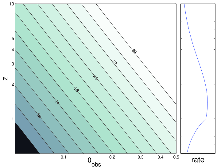
Figure 1: Left panel: R magnitude contour lines (from 17- left bottom to 29) for $F_{0}=0.003\,\mu{\rm Jy}$. The right panel depicts the GRB rate $n(z)(dV/dz)/(1+z)$ as a function of $z$ (for $z_{peak}=1$), as an indication to where we should expect most GRBs. As we plot only the region with $z>0.5$ the flux depends almost as a power law on the redshift.

According to our model an observer at $\theta_{obs}$ will observe the orphan afterglow if $\theta_{obs}<\theta_{max}(z,m)$. The afterglow will be detected over $t_{obs}(z,\theta,m)$:

$$t_{obs}(z,\theta,m)\approx{At_{jet}\over\theta_{j}^{2}}(\theta_{max}^{2}-\theta_{obs}^{2})$$ (12)

until the signal decays below the limiting magnitude. In this model which we denote model A, an orphan afterglow could be observed from a solid angle $2\pi[\theta_{max}(z,m)^{2}-\theta_{j}^{2}]$ where $\theta_{max}(z,m)$ does not depends on $\theta_{j}$. This model, and more specifically eq. 11, are quite generally valid for $\theta_{max}>\theta_{j}$. However if $\theta_{obs}\sim\theta_{j}$, $F_{\nu}^{max}(\theta_{obs})$ is more sensitive to the exact jet model being used. Specifically, in such a case there will be a significant contributions to the signal at $\theta_{obs}$ even before the jet’s opening angle reaches $\theta_{obs}$. This leads to a larger flux at $\theta_{obs}$ and hence to a larger $\theta_{max}$. For example, Granot et al. (2002) find, for their model II, that the solid angle between $\theta_{j}$ and the real maximal angle ($\tilde{\theta}_{max}$) is approximately constant even when $\theta_{obs}$ exceeds the asymptotic value of $\theta_{max}$ (given by equation 11), i.e. $\tilde{\theta}_{max}^{2}=\theta_{max}^{2}+\theta_{j}^{2}$. To take care of this effect we consider also model B, in which we assume that this relation holds. While model A is more conservative, model B allows for more orphan afterglows. We see later that for $m_{lim}\geq 25$ surveys, both models give comparable results. Model B gives a factor of 2.5 more orphan afterglows for $m_{lim}=23$ (with our ”canonical” parameters). It also predicts a larger ratio of orphan to on axis afterglows.

3 Results

The rate of observed orphan afterglows (over the entire sky) is (in model A):

$$R_{orph}=\int_{0}^{10}{n(z)\over(1+z)}{dV(z)\over dz}dz\int_{\theta_{j}}^{\theta_{max}(z,m)}\theta d\theta\ ,$$ (13)

where n(z) is the rate of GRBs per unit volume and unit proper time and dV(z) is the differential volume element at redshift $z$. We assume that the GRB rate is proportional to the SFR and is given by: $n(z)=B~{}10^{0.75z}$ for $z\leq z_{peak}$ and $n(z)=B~{}10^{0.75z_{peak}}$ for $z_{peak}<z<10$. The normalization factor, $B$, is found by the condition: $R_{GRB}^{true}=f_{b}R_{GRB}^{obs}=\int_{0}^{10}(dV/dz)n(z)/(1+z)dz$ where $f_{b}$ is the beaming factor and $R_{GRB}^{obs}=667\,{\rm yr}^{-1}$ . In the following we consider two star formation rates peaking at $z_{peak}=1$ and at $z_{peak}=2$ (Bouwenn, 2002).

Usually the detector’s exposure time is smaller than $t_{obs}(z,\theta,m)$. Thus, the number of detectable orphan afterglows in a single snapshot, over the whole sky, is:

$$N_{orph}=\int_{0}^{10}{n(z)\over(1+z)}{dV(z)\over dz}dz\quad\quad\quad\quad$$

$$\times\int_{\theta_{j}}^{\theta_{max}(z,m)}t_{obs}(z,\theta,m)\theta d\theta\ .$$ (14)

If we consider now model B we find:

$$R^{(B)}_{orph}={1\over 2}\left({F_{0}\over F_{lim}}\right)^{1/p}\quad\quad\quad\quad\quad\quad\quad$$

$$\times\int_{0}^{10}{n(z)\over(1+z)}{dV(z)\over dz}f(z)^{1/p}dz\ ,$$ (15)

where $F_{lim}$ is the limiting flux for detection. In this case $R_{orph}/R_{GRB}^{true}\sim(F_{0}/F_{lim})^{1/p}$ is independent of $f_{b}$. Using $t_{obs}(\theta_{obs})\approx t_{\theta}(\tilde{\theta}_{max})-t_{\theta}(\theta_{obs})$, we estimate the number of observed orphan afterglows:

$$N^{(B)}_{orph}={At_{jet}\over 4(1+z)\theta_{j}^{2}}\left({F_{0}\over F_{lim}}\right)^{2/p}\quad\quad\quad$$

$$\times\int_{0}^{10}n(z){dV(z)\over dz}f(z)^{2/p}dz\ .$$ (16)

We note that since $F_{0}\propto A^{-p}$ , both $R^{(B)}_{orph}$ and $N^{(B)}_{orph}$ scale as $1/A$.

The $z$ integrand of Eq. 14 gives the normalized redshift distribution of the observed orphan afterglows for model A (see Figure 2a). This distribution has a broad flat region all the way from $z=0$ to $z_{peak}$. It sharply declines above $z_{peak}$. For a SFR with a higher $z_{peak}$ there are significantly fewer orphan afterglows (see Figure 3). The function peaks (weakly) at $z_{peak}$ with higher limiting magnitude as more orphan afterglows are observed in this case. For model B the results are similar.

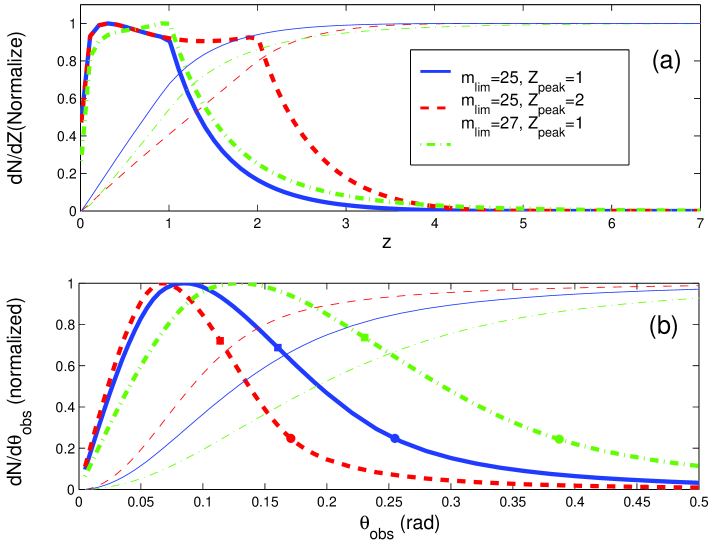
Figure 2: Top panel (a): the normalized redshift distribution of observed orphan afterglows in a single snapshot (thick lines) and the integrated $z$ distribution (thin lines). Bottom panel (b): the angular distribution of observed orphan afterglows in a single snapshot (thick lines) and the integrated $\theta_{obs}$ distribution (thin lines). The circles depict $\theta_{max}(z_{peak},m)$ and the squares depict $\langle\theta_{obs}\rangle$. In both panels we use $F_{0}=0.003\,\mu$Jy, and $\theta_{j}=0.1$. The different curves correspond to $m_{lim}=25$, $z_{peak}=1$ (solid line); $m_{lim}=25$, $z_{peak}=2$ (dashed line); $m_{lim}=27$, $z_{peak}=1$ (dashed-dotted line) and $m_{lim}=27$, $z_{peak}=2$ (dotted line).

The $\theta$ integrand of Eq. 14 [with $\theta_{max}(z,m)$ replaced by $z_{max}(\theta,m)$ and integration performed over $z$] yields the angular distribution for model A (see Figure 2b). For 25th limiting magnitude the median observing angle is $5^{\circ}$-$7^{\circ}$ depending on the SFR rate. With lower $z_{peak}$ most GRBs are nearer and hence stronger and detectable to a slightly larger angles. These values are close to the jet opening angles. Most of the observed orphan afterglows with this limiting magnitude will be “near misses” of on-axis events. The $\theta_{max}(z_{peak})$ are significantly larger ($10^{\circ}$ and $14^{\circ}$ respectively). With 27th magnitude the median of the angular distribution moves way out to $12^{\circ}$. This is larger than most GRB beaming angles but still narrow, corresponding only to 2% of the sky. Again the results for model B are similar (as long as $\theta_{j}\lesssim 0.1$).

As the sky coverage of GRB detectors is not continuously $4\pi$ it is possible that a GRB pointing towards us (i.e. with $\theta_{obs}<\theta_{j})$ will be missed, but its on-axis afterglow will be detected. In Table I we provide the ratio of the number of orphan afterglows to total number of afterglows (both on-axis and orphan), in a single snapshot of the sky. As expected this ratio is large for small jet opening angles and for large limiting magnitudes (and models A and B give similar results in this limit) and it decreases with increasing $\theta_{j}$ and decreasing $m_{lim}$. An insensitive search ($m_{lim}=23$) yields for model A, a comparable (or even larger) probability that a visual transient is a missed on-axis GRB whose afterglow is detected or an orphan one. However, for model B, this ratio is less sensitive to either $\theta_{j}$ or $m_{lim}$ for $\theta_{j}\sim\theta_{max}$, and even for $m_{lim}=23$ the majority of the afterglows would be orphans.

$z_{peak}$	$\theta_{j}$	$m_{lim}=23$	$m_{lim}=25$	$m_{lim}=27$
1	0.05	0.76 (0.81)	0.88 (0.90)	0.95 (0.95)
1	0.10	0.4   (0.63)	0.64 (0.73)	0.81 (0.84)
1	0.15	0.2   (0.55)	0.4   (0.63)	0.64 (0.74)
2	0.10	0.2   (0.56)	0.44 (0.64)	0.69 (0.76)

Table 1: Table I: The ratio of the number of orphan afterglows to the total number of afterglows (both on-axis and orphan), in a single snapshot, for different limiting magnitudes and jet opening angles. The first value is for model A, while the second one in brackets is for model B.

Figure 3 depicts the number of orphan afterglows per square degree (and in the entire sky), in a single exposure, as a function of the limiting magnitude. The thick lines are for model A (with various parameters) while the thin lines are for model B. In the “optimistic” case ($F_{0}=0.015\,\mu{\rm Jy}$, $\theta_{j}=0.05$) the predictions of both models are similar. With the “canonical” normalization ($F_{0}=0.003\,\mu{\rm Jy}$, $z_{peak}=1$ and $\theta_{j}=0.1$) model B predicts 2.5 times more orphan afterglows than model A, for a limiting magnitude of 23. These numbers provide an upper limit to the rate in which orphan afterglows will be recorded as point-like optical transients in any exposure with a given limiting magnitude. These numbers should be considered as upper limits, as our estimates do not include effects such as dust extinction that could make these transients undetectable.

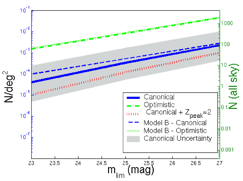
Figure 3: The number of observed orphan afterglows per square degree (left vertical scale) and in the entire sky (right vertical scale), in a single exposure, as a function of the limiting magnitude for detection. The thick lines are for model A with three different sets of parameters: i) Our “canonical” normalization $F_{0}=0.003\,\mu{\rm Jy}$, $z_{peak}=1$, $\theta_{j}=0.1$ (solid line). The gray area around this line corresponds an uncertainty by a factor of 5 in this normalization. ii) Our most optimistic model with a relatively small $\theta_{j}=0.05$ and a large $F_{0}=0.015\,\mu{\rm Jy}$ (dashed-dotted line). iii) The same as our “canonical” model, except for $z_{peak}=2$ (dotted line). The thin lines are for model B, where the solid line is for our “optimistic” parameters, while the dashed line is for our “canonical” parameters. Both models are similar for the “optimistic” parameters while model B predicts slightly more orphan afterglows then model A for the “canonical” parameters.

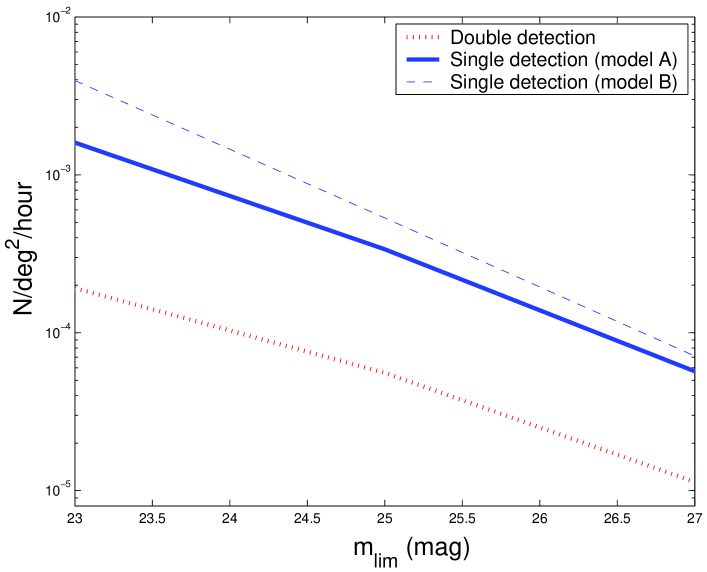
Figure 4: The detection rate of orphan afterglows per square degree per hour of telescope time. The curves that correspond to the “canonical” normalization are for a single detection in model A (solid line), a single detection in model B (dashed line) and a double detection in model A (dotted line). The rate is calibrated for a telescope that reaches $m_{lim}=25$ in a one hour exposure. It can be scaled up or down for other telescopes.

We ask now what will be the optimal strategy for a given observational facility: short and shallow exposures that cover a larger solid angle or long and deep ones over a smaller area. The exposure time that is required in order to reach a given limiting flux, $F_{lim}$, is proportional to $F_{lim}^{-2}$. We can now divide the number density of observed orphan afterglows (shown in Figure 3) by this time factor and obtain the rate per square degree per hour of observational facility. Figure 4 depicts this rate with a calibration to a hypothetical 2m class telescope that reaches a 25th magnitude with one hour exposure. Other telescopes will have another normalization but the trend seen in this figure remains. Figure 4 shows that shallow surveys that cover a large area are preferred over deep ones (in both models). This result can be understood as follows. Multiplying eq. 16 by $F_{lim}^{2}$ shows that the rate per square degree per hour of observational facility $\propto F_{lim}^{2-2/p}$. As $p>1$ ($2-2/p>0$) a shallow survey is preferred. A practical advantage of this strategy is that it would be easier to carry out follow up observations with a large telescope on a brighter transient detected in a shallow survey. Additionally one can expect that the number of spurious transients will be smaller in a shallower survey. However, if one wishes to detect orphan afterglows, one should still keep the surveys at a limiting magnitude of $\sim 23$, as for smaller magnitudes the number of on-axis transients detected will be comparable to (model B) or even larger than (model A) the number of orphan afterglows (see Table I).

The number density of orphan afterglow transients, given by Eq. 14 and depicted in Figure 3 gives an indication of the number of single events recorded above a limiting magnitude. Clearly, a single detection is not enough in order to identify that the transient indeed corresponded to an afterglow. A second following detection of the transient with a decrease by, say, 1 magnitude, would increase the probability that the transient is an orphan afterglow. We estimate the rate of a double detection of this nature by an afterglow search with a limiting magnitude $m_{lim}$ and a time delay $dT_{obs}$ between the two exposures of the same region in the sky. We consider, therefore, a detection of a transient in one exposure and a second detection after time $dT_{obs}$ in which the transient has decayed by more than one magnitude but is still above the limiting magnitude of the survey. This is of course an idealized situation and we do not consider realistic observational problems (like weather etc.) which may make the detection rate lower. Not surprisingly, the ratio of a double detection to a single detection depends on the time delay, $dT_{obs}$ (see Figure 5). The optimal time delay is the time in which an afterglow from $z_{peak}$ and with $m_{lim}$ decays by one magnitude: $dT_{obs}=3$ days for $m_{lim}=23$, $dT_{obs}=4$ days for $m_{lim}=25$ and $dT_{obs}=8$ days for $m_{lim}=27$. With this optimal choice, the fraction of the detected transients that will be detected in a second exposure, is 20% for $m_{lim}=27$ and 12% for $m_{lim}=23$. Note however, that the curve becomes narrower for low limiting magnitudes, making the exact timing of the second exposure more critical. Deeper surveys are less sensitive to the choice of the time delay.

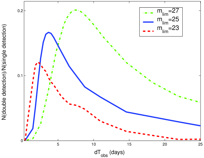
Figure 5: The ratio of double detection of orphan afterglows to a single detection, as a function of the time delay, $dT_{obs}$, between the two exposures. The three models are: $F_{0}=0.003\,\mu{\rm Jy}$, $z_{peak}=1$ and $m_{lim}=23$ (dashed line) $m_{lim}=25$ (solid line) and $m_{lim}=27$ (dashed-doted line).

It is interesting to compare the rate of observed orphan afterglows to the true GRB rate as a function of the beaming factor, $f_{b}\approx 2/\theta_{j}^{2}$. At this point models A and B differ the most. For model B this ratio is $\propto(F_{0}/F_{lim})^{1/p}$ and for the “canonical” parameters it holds the values of $0.004,0.014,0.031$ for $m_{lim}=23,25,27$ independently of $f_{b}$. In model A this ratio vanishes for low $f_{b}$ values. For high $f_{b}$ values the ratio converges to model’s B constant ratio. For the “canonical” parameters this ratio in model A reaches half of the asymptotic value for $f_{b}>50,125,250$ for $m_{lim}=27,25,23$ respectively. Thus, for strong beaming (or high $m_{lim}$) it is possible to estimate the true GRB rate from a determination of the orphan afterglow rate. For a low beaming factor this ratio is model dependent.

4 Discussion

We have calculated the number per unit solid angle of orphan afterglows that could be detected by idealized surveys with different limiting magnitudes. Our calculations are based on a simple idealized model for the hydrodynamics of the sideways expanding jets. Light curves from other models, including numerical simulations (Granot et al., 2001) described in Granot et al., (2002) show similar behavior. As the models differ when $\theta_{obs}\sim\theta_{j}$ we also consider an alternative assumption for this range. This yields analytic expressions for $R_{orph}$ and $N_{orph}$ (equations 15 and 16). We have shown that both models yield similar results for surveys deeper than $m_{lim}=25$ and have minor differences for surveys with $m_{lim}\sim 23$.

The normalization factor, $F_{0}$, of this light curve (Equation 11) is somewhat sensitive to the choice of the model parameters. Even observed afterglows with a clear jet break do not yield a well defined normalization factor, $F_{0}=A^{-p}f(z)^{-1}\theta_{j}^{2p}F_{\nu}(t_{jet},\theta_{obs}=0)$, because of the uncertainties in $\theta_{j}$, $A$, and $F_{\nu}(t_{jet},\theta_{obs}=0)$. As $N_{orph}\propto AF_{0}^{2/p}\propto F_{\nu}(t_{jet},\theta_{obs}=0)^{2/p}/A$ (equation 16), we expect the uncertainty in $N_{orph}$ to be similar to that in $F_{0}$ (a factor $\sim 10$). However, this uncertainty does not influence the trends that indicate a strategy for optimal orphan afterglow survey.

We stress that we do not consider here practical observational issues, such as dust extinction or the ability to identify a weak transient on top of a background host galaxy. We have also assumed idealized weather conditions: when considering a “verified” identification by two successive detections we assumed that a second exposure is always possible. All these factors will reduce the observed rate by some unknown factors below our optimistic values. We do not consider how recorded transients could be identified as afterglows. For example when we discuss a single detection we mean a single photometric record of a transient in a single snapshot. This is of course a very weak requirement and much more (at least a second detection) would be needed to identify this event as an afterglow.

Finally one should be aware of the possible confusion between orphan afterglows and other transients. Most transients could be completely unrelated (such as supernovae or AGNs) and could be distinguished from afterglows with followup observations. However, there could be a class of related transients like on-axis jets whose gamma-ray emission wasn’t observed due to lack of coverage or failed GRBs (Huang et al. 2002). The only quantitative measure that we provide is for the ratio of on-axis afterglows to truly orphan ones (i.e. off-axis afterglows whose prompt gamma-ray emission would have been detectable if viewed from within the jet opening angle).

We have shown that for a given dedicated facility the optimal survey strategy will be to perform many shallow snapshots. However, those should not be too shallow as we will observe more on-axis afterglows than off-axis ones. A reasonable limiting magnitudes will be $\sim 23-25$. With this magnitude we should perform a repeated snapshot of the same region after 3 to 4 days.

We consider now several possible surveys. The SDSS (York, 2000) has $m_{lim}\sim 23$ over $10^{4}$ square degrees in the north galactic cap. Figure 3 suggests that under the most optimistic condition we expect 15 detection of orphan afterglow transients in the north galactic cap of the SDSS. A careful comparison of the SDSS sky coverage and the exposure of relevant GRB satellites could reveal the rate of coincident detection (GRB - Sloan optical transient) from which one could get a better handle (using Table I) on the possible rate of detection of orphan afterglows by SDSS. Under the more realistic assumptions we expect a single orphan afterglow transient in the SDSS. Note that the 5 filters SDSS system could possibly select orphan afterglow candidates even with only a single detection (Rhoads 2001; Vanden Berk et.al, 2001), though this method could be applied only to bright sources. As the north galactic cap survey provides only a single snapshot with no spectral information at magnitude of 23, even if a transient will be recorded in this survey it will be impossible to identify it as a transient. Clearly this is not the best survey for orphan afterglows search. However, The south galactic cap survey, observes the same part of the sky repeatedly with $m_{lim}\sim 23$. It can achieve a higher magnitude, 25th, for steady sources. If the repetition interval is longer than 2 weeks, than for most orphan afterglows, the second observations can be considered as a new one. Therefore, given that the time spent in the south cap is comparable to the time spent in the north cup, the detection rate should be comparable. The Advantage of the south cap is the ability to identify transients sources even if the decay process could not be observed, and the possibility of ruling out sources that are not transient in nature, such as AGNs.

Consider now a dedicated 2m class telescope with an aperture $0.5\Box^{\circ}$ of $m_{lim}=24$ for a 10 minutes exposure and $m_{lim}=25$ for a 1 hour exposure. Under our most optimistic assumptions it will record up to 35 orphan afterglows per year in the shallow mode and a third of that (13 afterglows) in the deeper mode. Using our “canonical” model we find two orphan afterglows per year in the shallow mode.

The VIMOS camera at the VLT has a comparable aperture of $0.06\Box^{\circ}$ but it can reach $m_{lim}=26$ in 10 minutes and $m_{lim}=27$ in an hour. A single $m_{lim}=27$ frame would have a $0.002$ orphan afterglows under the most optimistic assumptions ($1.1\cdot 10^{-4}$ canonically). Thus, at best 2-3 orphan afterglows should be hiding in every 1000 exposures. The Subaru/Suprime-cum has a similar sensitivity but its field of view is four times larger. Therefore every 1000 exposures should contain no more than 10 orphan afterglows.It will be however a remarkable challenge to pick up these transients and confirm their nature from all other data gathered in these 1000 exposures.

We thank Tom Broadhurst, Re’em Sari and Avishay Gal-Yam for helpful remarks. This research was supported by a US-Israel BSF grant and by NSF grant PHY-0070928.

References

- Broadhurst, (2002) Bouwenn, E. N. S., Broadhurst, T. J., & Illingworth, R. J., 2002, submitted.
- Dalal, Griest, & Pruet (2002) Dalal, N., Griest, K., & Pruet, J. 2002, ApJ, 564, 209.
- Frail et al. (2001) Frail, D. A. et al. 2001, ApJ, 562, L55.
- Granot et al. (2001) Granot, J., Miller, M., Piran, T., Suen, W. M., & Hughes, P. A. 2001, Gamma-Ray Bursts in the Afterglow Era, Proceedings of the International workshop held in Rome, CNR headquarters, 17-20 October, 2000. Edited by Enrico Costa, Filippo Frontera, and Jens Hjorth. Berlin Heidelberg: Springer, 2001, p. 312., 312.
- Granot (2002) Granot, J., Panaitescu, A., Kumar, P. & Woosley, S. E. 2002, ApJin press, astro-ph/0201322
- Granot & Sari (2002) Granot, J. & Sari, R. 2002, ApJ, 568, 820.
- Harrison et al. (2001) Harrison, F. A. et al. 2001, ApJ, 559, 123.
- Harrison et al. (1999) Harrison, F. A. et al. 1999, ApJ, 523, L121.
- Huang et al. (2002) Huang, Y.F., Dai, Z.G. & Lu, T. 2002, accepted to MNRAS (astro-ph/0112469)
- Panaitescu & Kumar (2001) Panaitescu, A. & Kumar, P. 2001, ApJ, 560, L49.
- Piran (1994) Piran, T. 1994, AIP Conf. Proc. 307: Gamma-Ray Bursts, 495.
- Piran (2000) Piran, T. 2000, Phys. Rep., 333, 529.
- Piran, Kumar, Panaitescu, & Piro (2001) Piran, T., Kumar, P., Panaitescu, A., & Piro, L. 2001, ApJ, 560, L167.
- Rhoads (1997) Rhoads, J. E. 1997, ApJ, 487, L1.
- Rhoads (1999) Rhoads, J. E. 1999, ApJ, 525, 737.
- Rhoads (2001) Rhoads, J. E. 2001, ApJ, 557, 943.
- Sari, Piran, & Narayan (1998) Sari, R., Piran, T., & Narayan, R. 1998, ApJ, 497, L17.
- Sari, Piran, & Halpern (1999) Sari, R., Piran, T., & Halpern, J. P. 1999, ApJ, 519, L17.
- Stanek et al. (1999) Stanek, K. Z., Garnavich, P. M., Kaluzny, J., Pych, W., & Thompson, I. 1999, ApJ, 522, L39.
- Vanden Berk et. al. (2001) Vanden Berk, D. et. al. 2001, astro-ph/0111054
- York et al. (2000) York, D. G. et al. 2000, AJ, 120, 1579.