Determining Central Black Hole Masses in Distant Active Galaxies.

Abstract

An empirical relationship, of particular interest for studies of high redshift active galactic nuclei (AGNs) and quasars, between the masses of their central black-holes and rest-frame ultraviolet (UV) parameters measured in single-epoch AGN spectra is presented. This relationship is calibrated to recently measured reverberation masses of low-redshift AGNs and quasars. An empirical relationship between single-epoch rest-frame optical spectrophotometric measurements and the central masses is also presented. The UV relationship allows reasonable estimates of the central masses to be made of high-redshift AGNs and quasars for which these masses cannot be directly or easily measured by the techniques applicable to the lower luminosity, nearby AGNs. The central mass obtained by this method can be estimated to within a factor of $\sim$3 for most objects. This is reasonable given the intrinsic uncertainty of a factor less than 2 in the primary methods used to measure the central masses of nearby inactive and active galaxies, namely resolved gas and stellar kinematics in the underlying host galaxy and reverberation-mapping techniques. The UV relationship holds good potential for being a powerful tool to study black-hole demographics at high redshift as well as to statistically study the fundamental properties of AGNs. The broad line region size $-$ luminosity relationship is key to the calibrations presented here. The fact that its intrinsic scatter is also the main source of uncertainty in the calibrations stresses the need for better observational constraints to be placed on this relationship. The empirically calibrated relationships presented here will be applied to quasar samples in forthcoming work.

To appear in the Astrophysical Journal, June 1, 2002 The Astrophysical Journal, June 1, 2002

1 Introduction and Motivation

The mass of the central black hole, $M_{\rm BH}$, is a fundamental property of active galactic nuclei (hereafter AGNs) and quasars governing the physics of their central engine. The mass of the central black hole (or “massive dark object”) can be measured in nearby, inactive galaxies using gas and stellar kinematics (e.g., Kormendy & Richstone 1995; Richstone et al. 1998; Ho 1999; Kormendy & Gebhardt 2001) and in nearby, active galaxies using results from reverberation mapping studies (e.g., Koratkar & Gaskell 1991; Peterson & Wandel 1999, 2000; Ho 1999; Wandel, Peterson, & Malkan 1999; Kaspi et al. 2000). Recent developments have shown the central mass in both inactive and active galaxies to be related to properties of its host galaxy, namely the bulge luminosity $L_{\rm bulge}$, (inactive galaxies: e.g., Kormendy & Richstone 1995; Magorrian et al. 1998; Richstone et al. 1998; Ho 1999; active galaxies: e.g., Laor 1998; Ho 1999; Wandel 1999; see also Laor 2001; McLure & Dunlop 2001; Wandel 2001) and the bulge stellar velocity dispersion, $\sigma$ (inactive galaxies: Ferrarese & Merritt 2000; Gebhardt et al. 2000a; see also Merritt & Ferrarese 2001a; active galaxies: Gebhardt et al. 2000b; Ferrarese et al. 2001). This is indicative of related formation processes of the central mass and the bulge in the host galaxy. The reasons for these purely empirical relationships, and that the $M_{\rm BH}$ $-$ $\sigma$ relationship is tighter than the $M_{\rm BH}$ $-$ $L_{\rm bulge}$ relationship, are not clear, but several attempts to explain them exist (e.g., Silk & Rees 1998; Haehnelt & Kauffmann 2000; Adams, Graff, & Richstone 2001; Burkert & Silk 2001; see also § 5 of Merritt & Ferrarese 2001b). Further study of these relationships and how they may change with redshift is one of many motivations for studying supermassive black holes at high redshift.

Spatially resolved gas and stellar kinematical studies are most useful for measuring central masses in inactive and weakly active galaxies. This is because in AGNs the strong glare from the central non-stellar continuum source inhibits measurements of the stellar absorption features, and the narrow-line gas kinematics are perturbed by non-gravitational forces. Reverberation (or echo-) mapping techniques (e.g., Blandford & McKee 1982; Peterson 2001a) do not require high spatial resolution but instead utilize the intrinsic continuum source variability and light travel time delays between the location of the ionizing continuum source and the line-emitting gas responding to the changing continuum. If the line-emitting gas is gravitationally bound to the central black hole, then simple virial arguments imply that the central mass can be measured. Reverberation analysis techniques have in recent years been improved to provide reasonable estimates of the size of the broad line region (BLR) and thereby to provide reasonable central mass estimates. The accuracy of size determinations depend on the data quality, temporal sampling, duration of the monitoring campaigns (Collier, Peterson, & Horne 2001; Polidan & Peterson 2001), and analyses techniques (e.g., Peterson et al. 1998b; Welsh 1999; see also Horne 2001). Work is in progress to reanalyze the available AGN Watch data with better analysis techniques to improve the central mass estimates for the Seyfert 1 galaxies which currently have large uncertainties (B. M. Peterson 2001, private communication). Ferrarese et al. (2001) discuss the cause of these large errors. The simple underlying idea of echo mapping is that the measured time delays and the behavior and properties of the varying continuum and line emission indeed measure distances and velocity dispersion in the BLR and thus measure the central mass with reasonable accuracy. This assumes that the black hole gravity dominates radiation pressure effects on the BLR and evidence in favor of this now exists (Gaskell 1988; Peterson & Wandel 2000; Gebhardt et al. 2000b; Ferrarese et al. 2001). Arguments have been presented that it is to be expected, theoretically, that other processes than gravity, such as radiation pressure, anisotropic emission, and projection effects, should introduce large systematic uncertainties which dominate and prevent accurate measurements of the central masses (Krolik 2001). It is worth keeping in mind that theoretical considerations are equally affected by our limited knowledge on the geometry and the details of the kinematics in the central regions of AGNs. This seems founded by the recent studies, which find good consistencies in the central masses of nearby AGNs measured both with reverberation and stellar kinematical techniques (Gebhardt et al. 2000b; Ferrarese et al. 2001).

Central masses can now be determined with much smaller uncertainties (less than a factor of 2 depending on the method and data quality) than the early crude estimates could provide (e.g., Dibai 1980; Wandel & Yahil 1985; Wandel & Mushotzky 1986; Padovani & Rafanelli 1988; Padovani, Burg, & Edelson 1990). The accuracy of reverberation mass determinations may further improve given the continuously improving reverberation analyses techniques. These recent developments allow us to revisit with modern techniques fundamental issues such as how AGN supermassive black holes evolve and relate to galaxy formation and evolution (e.g., Richstone et al. 1998; Fabian 1999; Kauffmann & Haehnelt 2000). While reverberation techniques and stellar and gas kinematical studies will yield valuable insight to the local black-hole demography, the situation is different for high-redshift AGNs. In principle, the $M_{\rm BH}$ $-$ $\sigma$ relationship is sufficiently tight to allow estimates of the central AGN mass based on the measured velocity dispersion, $\sigma$, of the central host galaxy spectrum. This requires, however, a significant host galaxy contribution in the AGN spectrum. At the time of writing this can only be efficiently studied for low-luminosity, nearby AGNs (e.g., Nelson & Whittle 1995; Ferrarese et al. 2001). Reverberation mapping techniques can in principle be applied to distant AGNs. Unfortunately, such studies are also very telescope- and time-consuming (e.g., Peterson 2001a,b), especially for the more distant and fainter AGNs and for the (intrinsically) more luminous quasars, which vary on longer time scales (e.g., Kaspi 2001). The method is also highly dependent on the objects actually showing intrinsic continuum luminosity variations when observed. As a result, obtaining accurate reverberation mapping masses of a large, representative sample of the distant AGN and quasar populations is close to impossible in a human lifetime. Nevertheless, significant advances can be made with reasonable estimates of the central black hole masses in these objects even to within a factor of a few. This is particularly useful if the mass estimates are based on data that are relatively easy to obtain such as a single-epoch spectrum. The best available approach is likely the “ladder” type of calibration, known from the distance scale determination (e.g., Freedman et al. 2001). That is, one calibrates appropriate parameters, more easily obtained for higher redshift objects, to the mass measurements at low-$z$. Such an approach is pursued here. A relationship between $M_{\rm BH}$, the H $\beta$ line width, and the optical continuum luminosity, $L_{\lambda}$(5100Å), is already established [see eqns. (1) and (2) later] through the confirmation of the theoretically expected relationship between the BLR size, $R_{\rm BLR}$, and $L_{\lambda}$(5100Å) [Wandel et al. 1999; Kaspi et al. 2000]. The time delay, $\tau$, and hence $R_{\rm BLR}=c\tau$ for C iv $\lambda$ 1549 is about half that of H $\beta$ (Korista et al. 1995), and multiple broad emission lines in NGC 5548 exhibit the same virial relationship (Peterson & Wandel 1999, 2000), as expected if reverberation techniques work. Therefore, it is reasonable to assume that a similar relationship can be obtained with appropriate rest-UV spectral measurements. Such a relationship is of particular interest if single-epoch spectra can supply the required rest-frame UV measurements. Then it becomes straightforward to estimate central masses for large samples of high-redshift AGNs. If uncertainties in such an approach are, relatively speaking, reasonable this is a powerful tool for statistical studies and black hole demography at high redshift. This is the focus of this paper.

The C iv $\lambda$1549 emission line is chosen here to provide a characteristic velocity dispersion appropriate for the calibration of single-epoch UV spectral measurements for several reasons. First, this line is accessible from the ground for objects with redshifts between $\sim$1 and $\sim$5. Second, its profile is not commonly affected by strong or numerous absorption lines typical of the Ly $\alpha$  emission line. Also, its line width is also much less affected by blending effects from other line emission, including Fe ii emission, than either of the C iii] $\lambda$1909 and Si iv+O iv] $\lambda$1400 lines. Contaminating Fe ii and He ii $\lambda$1640 emission mainly affect the lower profile wings of C iv (e.g., Figure 2 by Marziani et al. 1996; Vestergaard & Wilkes 2001; M. Vestergaard et al., in preparation). For these reasons it is also an emission line on which future rest-frame UV and optical reverberation mapping analyses may be applied in both nearby and more distant AGNs, providing tests of the calibrations presented here.

It is important to point out that such calibrations do not eliminate the need for further reverberation mapping studies. Rather, they emphasize the strong need to obtain yet better and more monitoring data. First, this work and the BLR size – luminosity relationship are based on samples of Seyferts and quasars that are, after all, small ($\stackrel{{\scriptstyle\scriptscriptstyle<}}{{\scriptstyle{}_{\sim}}}$34 objects) and do not span the full range of observed AGN properties. Second, the UV and optical calibrations presented in this work depend strongly on the size $-$ luminosity relationship and the intrinsic scatter around this relationship is the main source of uncertainty in the calibrations (§ 5 and § 6). The presence of this scatter thus accentuates the need for more and better BLR size determinations. It is now quite clear that significant improvements thereof require and can be obtained by a fully dedicated set of space-based telescopes, which can provide sufficient temporal sampling and duration of the monitoring campaigns (Collier et al. 2001), and simultaneous observations across multiple wavelength bands (Peterson 2001b; Netzer 2001) to constrain the transfer functions and the BLR geometry better. In return, more accurate measurements can be obtained of the BLR size, and hence of the central masses (e.g., Horne et al. 2002). This is just one of the important issues that the proposed MIDEX mission, Kronos, will address if selected. Given the practical difficulties of long term multi-wavelength monitoring with existing facilities on the ground and in space (HST and X-ray telescopes), including obtaining bona-fide simultaneous observing time on many different telescopes for long periods of time, Kronos may quite possibly be our best opportunity to study how the central regions of nearby and distant AGNs are structured and “engineered” (Blandford 2001). Ultimately, that will allow more accurate mass estimates for distant AGNs than are possible at present, as discussed above.

This work was inspired by the recently established BLR size $-$ luminosity relationship (Kaspi et al. 2000), which is applicable not only for nearby Seyfert 1 galaxies but also for the intrinsically brighter quasars. Hence, assuming this size $-$ luminosity relationship applies to more distant quasars also, their central masses can thus be estimated. Here, relationships between $M_{\rm BH}$ and single-epoch rest-frame optical and UV measurements, respectively, are derived and the uncertainties introduced by this approach are evaluated. It will be shown that single-epoch spectrophotometry can be used to estimate the central masses to within a factor of 3 with high probability, rendering the calibrations very useful.

In what follows ‘optical’ and ‘UV’ refer to these same bands in the rest-frame of the AGN or quasar. A cosmology with H₀ = 75 ${\rm km~{}s^{-1}Mpc^{-1}}$, q₀ = 0.5, and $\Lambda$ = 0 is used throughout.

The paper is structured as follows. The method adopted for the calibration is outlined in § 2. Section 3 describes the data considered, § 4 discusses how well representative the single-epoch optical data are of the multi-epoch reverberation data, §§ 5 and 6 present calibrations of single-epoch optical and UV measurements, respectively. In § 7 the performance of the adopted calibrations is evaluated.

2 The Method

The virial theorem is used to estimate the mass of the central black hole, $M_{\rm BH}\approx rv^{2}/G$, where $v$ is the velocity dispersion of matter at distance, $r$, which is gravitationally bound to the black hole. The velocity dispersion can be expressed as $v=f\,\cdot v_{\rm FWHM}$ where $v_{\rm FWHM}$ is the FWHM of the emission profile of the broad line gas. The factor $f$ is on the order of unity and depends on the geometry and the details of the kinematics (e.g., Peterson & Wandel 1999, 2000; Fromerth & Melia 2000; Krolik 2001; McLure & Dunlop 2001). The central mass can be expressed as:

$$M=1.5\times 10^{5}\left(\frac{R_{\rm BLR}}{\rm lt-days}\right)\left(\frac{v_{\rm FWHM}}{10^{3}~{}\rm km~{}s^{-1}}\right)^{2}\mbox{$M_{\odot}$}$$ (1)

Based on 17 nearby Seyfert 1 galaxies (Wandel et al. 1999) and 17 Palomar-Green (hereafter PG; Schmidt & Green 1983; Green, Schmidt, & Liebert 1986) quasars, Kaspi et al. (2000) determine an empirical relationship between the size of the broad line region, $R_{\rm BLR}$, and the continuum luminosity, $\lambda L_{\lambda}$(5100Å), where $R_{\rm BLR}$ is the distance of the emission-line clouds responding to the central continuum variations as determined from reverberation studies [eq. (6) of Kaspi et al. 2000]:

$$R_{\rm BLR}=(32.9^{+2.0}_{-1.9})~{}\left[\frac{\lambda L_{\lambda}\rm(5100\AA)}{10^{44}~{}\rm~{}ergs\,s^{-1}}\right]^{0.700\,\pm\,0.033}~{}~{}{\rm lt-days}$$ (2)

In appendix A this relationship is re-derived using regression analysis appropriate for data with internal scatter. A critical assessment of the object sample is also performed. The modified luminosity dependence has a larger uncertainty, which is probably more realistic given the intrinsic scatter, than that quoted above. However, within this uncertainty the approach adopted in appendix A does not yield an $R_{\rm BLR}-L$ relationship significantly different from that of Kaspi et al. for the current sample of AGNs; this may change once more data are available to better constrain the $R_{\rm BLR}-L$ relationship. Therefore, in what follows eqn. (2) is used to estimate the BLR size when unknown.

Equation (1) assumes that the broad line emitting gas is gravitationally bound, and that the cloud velocity dispersion is isotropic such that $v\,=\,\sqrt{3}\,|\sigma_{i}|,~{}i\,=\,1,2,3~{};~{}|\sigma_{i}|\,=\,v_{\rm FWHM}$/2; $v_{\rm FWHM}$ is in units of km s^-1. The details of the geometry and kinematics, i.e., the exact value of $f$, are unknown but have been debated (e.g., Peterson & Wandel 1999; Fromerth & Melia 2000; McLure & Dunlop 2001). Most expected values of $f$ are anticipated to result in a constant offset in $\log$ $M_{\rm BH}$ (Krolik 2001). Because such details are not yet clarified or well constrained (e.g., Wandel 2001) the approach taken in this work is to compute the central masses with basic and common assumptions to allow comparison with most other work. The offsets in mass estimates due to different assumptions of geometry and kinematics should however be kept in mind when considering the $M_{\rm BH}$ values in absolute terms.

Assuming that equation (2) is valid for all active galaxies, we therefore have an approximative relationship between the mass of the central black hole, the AGN continuum luminosity at 5100Å and the line width of the H$\beta$ emission-line [eqn. (1)]. Given that the BLR size $-$ luminosity relationship is determined from line-continuum variability of the objects, the specific H $\beta$ line width to be used to determine the ‘reverberation mass’ is that appropriate for the emission-line gas at the distance $R_{\rm BLR}$ from the ionizing continuum source that is varying. That is, the FWHM of H $\beta$ in the ‘root-mean-square (rms) spectrum’ (e.g., Peterson & Wandel 1999, 2000) will be used below for the variability data. Kaspi et al. (2000) argue that FWHM(H $\beta$, mean), the FWHM of H $\beta$ in the ‘mean spectrum’, may equally well be used. In the interest of completeness and for comparison, the masses based on the mean optical spectra are included in the analysis below, even if the rms masses are considered, strictly speaking, the most representative of the intrinsic, actual central masses.

The method used here to calibrate single-epoch UV measurements to reflect the central black-hole masses is briefly as follows. First, the single-epoch FWHM(H $\beta$) and continuum luminosities are compared with the multi-epoch equivalents to test how representative the single-epoch measurements are, and whether systematic offsets between these two sets of measurements exist (§ 4). If that is the case, a calibration or modification of the single-epoch measurements may be appropriate to ensure they introduce minimum systematic error or do not add unnecessary scatter. Then, the single-epoch mass estimates based on optical measurements, $M_{\rm BH}(\rm H\beta)$, are computed using equations (1) and (2). These estimates are compared and calibrated to the available reverberation masses, $M_{\rm BH}(\rm H\beta,rms)$, based on H $\beta$ measurements for the PG quasars (§ 5). The next step is to determine the best calibration of an appropriate combination of the single-epoch FWHM(C iv) and $\lambda$ $L_{\lambda}$(1350 Å) measurements to the best available $M_{\rm BH}$ measurements (§ 6). This is done for the subset of 26 objects with both $M_{\rm BH}(\rm H\beta,rms)$ and UV measurements available. How well this method yields representative central mass estimates is discussed in § 7.

3 Data

The calibration of optical single-epoch spectral measurements is based on the 19 objects common to the sample of Seyfert 1s and PG quasars with established reverberation masses (Peterson & Wandel 1999, 2000; Wandel et al. 1999; Kaspi et al. 2000) and the PG quasars studied by Boroson & Green (1992; hereafter BG92). The calibration of the single-epoch UV measurements is based on the sample (labeled “UVrev”) of 26 reverberation AGNs and PG quasars (Wandel et al. 1999; Kaspi et al. 2000) with available UV spectroscopy. Mostly for comparison, a sample is also considered consisting of UVrev and 30 additional PG quasars (BG92) for which C iv line widths and UV continuum luminosities are also available in the literature. These data are described in the following.

3.1 Optical Data

BG92 list H$\beta$ FWHM measurements of single-epoch spectra of many quasars in the PG sample from which the contaminating iron emission and the narrow line contribution are subtracted; i.e. the FWHM is that of the supposedly intrinsically emitted broad H$\beta$ line emission. Some of the line widths were substituted with measurements obtained in this work, because the subtraction of the narrow component renders the profile less representative of the line width needed for this study (§ 4.1).

Monochromatic luminosities, $L_{\lambda}$ (5100Å), are determined for most of the PG quasars from the spectrophotometry by Neugebauer et al. (1987). The flux densities at 5100Å are approximated by a linear interpolation. For most objects this interpolation is done over short or neighboring frequency ranges in relatively tight spectral energy distributions, and so should be reliable. For the few sources not included in this database $L_{\lambda}$(5100Å) is computed based on the 4400 Å flux densities listed by Kellerman et al. (1989). These are based on B-band photometry of Schmidt & Green (1983). A power-law continuum, F${}_{\nu}\propto\nu^{\alpha}$, with an average optical slope, $\alpha~{}=~{}\alpha_{\rm opt}$ = $-$0.5 is assumed and extrapolated to 5100 Å. The optical data are listed in Table Determining Central Black Hole Masses in Distant Active Galaxies..

Errors on the parameters are propagated using the following assumed uncertainties: (1) spectral slopes, $\sigma(\alpha)$=0.2, reflecting the different slopes commonly adopted in the literature for quasars (e.g., Francis et al. 1991: $\alpha$=$-$0.3; Véron-Cetty & Véron 1993: $\alpha$=$-$0.7), (2) redshift, $\sigma(z)$=0.0025, a compromise between the typical uncertainty for redshift determinations based on optical and low-ionization lines, and those relying on UV high-ionization lines only where velocity shifts may exist between lines, especially for higher redshift quasars [$\sigma(z)$ has a negligible effect], (3) Neugebauer et al. (1987) quote flux errors for each measurement and for each object, and (4) the B-magnitude uncertainty is 0.27 mag (Schmidt & Green 1983). BG92 do not quote the uncertainty on their FWHM(H $\beta$) measurements. Based on the few error quotes available in the literature (e.g. Brotherton 1996; Vestergaard 2000; M. Vestergaard et al. , in preparation) a reasonable relative error on the FWHM measurements of broad emission lines is $\sim$10% depending on the measurement method and the quality of the data. Blending effects will increase this uncertainty. The uncertainties in the BLR size $-$ luminosity relationship [eqn. (2)] are also taken into account; see also Appendix A.

3.2 UV Data

The single-epoch UV measurements were obtained from a handful of studies including Wilkes et al. (1999), Wang, Lu, & Zhou (1998), Laor et al. (1994, 1995), Koratkar & Gaskell (1991), and Wills et al. (1995). Line widths and luminosities were generally taken from the same study. For a few objects with data only presented by Marziani et al. (1996) the line widths were remeasured directly on the published C iv profiles. This was done because the authors decompose the profiles and only list measurements for the individual broad and narrow components. As argued in § 4.1 the line widths for this study should be measured on profiles including the narrow component as it originates in the BLR like the broad component; this is contrary to the assumption of Marziani et al. (1996). Most of these earlier studies present UV continuum luminosities at 1350Å or quite close to it. Wilkes et al. (1999) quote continuum luminosities at 2500 Å, extrapolated from available V and B band photometry. Most of the objects studied by Wilkes et al. were also studied by others who do measure the continuum luminosities directly. These latter measurements are less subject to extrapolation uncertainties and were thus preferred. All the luminosities adopted from the literature were extrapolated to be a measure of the 1350 Å luminosity, if necessary, assuming the slope and cosmology quoted above; this extrapolation is in all cases over a relatively short wavelength range ($\stackrel{{\scriptstyle\scriptscriptstyle<}}{{\scriptstyle{}_{\sim}}}$100 Å). For the measurements with quoted uncertainties the errors were propagated, as outlined above. For line widths with no measurement errors a conservative uncertainty of 10% was imposed. Typical luminosity uncertainties of 30% were adopted for luminosities without quoted errors. The discussion in § 4.2 show this is reasonable.

For some of the objects two or more studies quote line widths and luminosities. It was then assumed that the differing measurements is a consequence of intrinsic scatter due both to variability and to measurement uncertainty. The mean of the measurements was therefore adopted and the difference in line width was adopted as the uncertainty in the FWHM measurement, unless it was smaller than the adopted conservative 10% error. The luminosities were generally rather similar. The adopted UV measurements and their source references are listed in Table Determining Central Black Hole Masses in Distant Active Galaxies..

4 Calibration of Single-Epoch Optical Measurements

Before the single-epoch spectral measurements (line width and monochromatic luminosity) are calibrated to the (multi-epoch) reverberation measurements it is important to compare these two types of measurements to examine whether single-epoch measurements are reasonably representative of the reverberation measurements, to what degree and whether certain spectral corrections are necessary. This includes an attempt to understand how and in what way they may differ. This direct comparison is performed on the objects common to the Kaspi et al. (2000) and BG92 studies, namely the 17 PG quasars studied by Kaspi et al. and two Seyfert galaxies, Mrk 110 and Mrk 335, (Wandel et al. 1999), all of which were studied with reverberation mapping techniques.

4.1 Line Width Measurements

The appropriate BLR velocity dispersion to use in the mass estimate is that measured from the ‘rms’ profile (§ 2). Because the mass depends strongly on the line width [eqn. 1] it is important to identify the single-epoch line profile that best represents the rms profile. That is, is it important to subtract contaminating Fe ii emission, and/or perhaps the narrow line contribution before measuring the FWHM? Another goal of this section is to quantify how well a single-epoch line width measurement estimates the rms line width. Rms spectra show the variable part of the continuum and line emission and its strength as a function of wavelength. The H $\beta$ line width in the rms spectrum, hereafter FWHM(H $\beta$, rms), is the width of the variable part of the line. Rms spectra can have different line emission contribution from single-epoch spectra (examples of mean and rms profiles are presented by Peterson et al. 1998a). The H $\beta$ line width measured in a single-epoch spectrum, hereafter FWHM(H $\beta$), is expected to be more similar to the mean of many individual (single-epoch) spectra than FWHM(H $\beta$, rms), which depends on which part of the broad line gas that varies. Therefore, in what follows, after a general discussion of the single-epoch and multi-epoch line widths, the FWHM(H $\beta$) values are first discussed in relation to FWHM(H $\beta$, mean) and then to FWHM(H $\beta$, rms).

4.1.1 The Best Single-Epoch Profile to Measure

Figures 8a and 8b show the FWHM(H $\beta$, mean) and FWHM(H $\beta$, rms), respectively, and their uncertainties measured by Kaspi et al.  and Wandel et al.  in their multi-epoch spectra are plotted for the 18 objects of those mentioned above with H $\beta$ measurements versus the single-epoch FWHM(H $\beta$) measurements by BG92. Note that there is a typographical error in Table 2 of BG92, FWHM(H $\beta$) = 5320 km s^-1 for PG1307$+$085 (Laor 2000). The dotted line represents a one-to-one relationship. With a few exceptions (labeled in Fig. 8) the single-epoch FWHM(H $\beta$) shows a general consistency with FWHM(H $\beta$, mean) within 15% $-$ 20% variation in the single-epoch width and also show consistency with FWHM(H $\beta$, rms) to within $\sim$20% $-$ 25% variation. This is consistent with the $\pm$15% line width variation (B. M. Peterson 2001, private communication) observed for NGC 5548 during 1988 December 14 $-$ 1996 October 16 (e.g., Peterson et al. 1999), where the H $\beta$ line flux varied up to $\pm$66%. It indicates that most of the single-epoch FWHM(H $\beta$) measurements and their deviation from the multi-epoch measurements can perhaps be accounted for as being due to intrinsic continuum and line variations. A detailed discussion of these deviations follows below.

It is important to note that there are technical differences between the BG92 and the multi-epoch measurements. BG92 fit and subtract the optical Fe ii emission around H $\beta$ and [O iii] $\lambda$$\lambda$4959, 5007 and also fit and subtract the narrow line H $\beta$ contribution. Kaspi et al. and Wandel et al. do not perform any of these corrections to their data. Subtraction of the narrow line contribution will increase the FWHM value. This increase may be quite significant depending on the strength of this contribution (see below and e.g., Jackson & Browne 1991). By eliminating the Fe ii emission, which blends into the red wing of H $\beta$ and both of the [O iii] doublet lines, a smaller H $\beta$ width is obtained. This holds as long as the contaminating Fe ii emission does not artificially increase the underlying continuum level significantly, creating a so-called “pseudo-continuum” (e.g., Wills, Netzer, & Wills 1985; Vestergaard & Wilkes 2001). Subtracting the Fe ii emission will then tend to increase the FWHM as the line peak height is increased (the local continuum level or “zero-point” of the line is lowered). Thus, the effects of subtracting the Fe ii emission is not straightforward to predict a priori.

For this type of study the FWHM(H $\beta$) measurement that best represents FWHM(H $\beta$, rms) is one measured on a profile for which only a correction for strong Fe ii contamination is performed, and especially one in which the narrow line contribution is not subtracted. This is justified in the following. Note that if the Fe ii emission is essentially constant in strength while the object was monitored, the Fe ii emission contribution is automatically eliminated in the rms spectra. AGN optical Fe ii emission does not seem to vary much or very fast if at all (e.g., Wamsteker et al. 1990; Kollatschny & Welsh 2001) so it is reasonable to assume that the FWHM(H $\beta$, rms) is not significantly affected by Fe ii emission, if present. For this reason it is desirable to use single-epoch FWHM(H $\beta$) measurements which are not affected by the presence of Fe ii emission.

For these reasons and because some of the BG92 FWHM(H $\beta$) measurements deviate strongly from the FWHM(H $\beta$,rms) of Kaspi et al. and Wandel et al. (see below and Fig. 8), the line width was remeasured in this work in the original spectra (i.e., those not corrected for Fe ii or narrow component emission; these data were kindly provided by T. Boroson) of the PG quasars studied by Kaspi et al. With exception of a handful of objects with strong Fe ii emission and/or a strong narrow line emission component, these non-corrected FWHM values are consistent with the BG92 values to within the (assumed) 10% measurement uncertainties; the inconsistent measurements were corrected as described below. The objects showing “uncorrected” FWHM(H $\beta$) values larger than the BG92 measurements are all Fe ii-strong, indicating that the Fe ii blending effects in the red wing of H $\beta$ dominate the effects of the alleged Fe ii-pseudo-continuum for these objects. For these objects the Fe ii corrected BG92 measurements were chosen to be the most representative of FWHM(H $\beta$, rms) since this width is not significantly affected by Fe ii emission. However, the uncertainties of the BG92 FWHM(H $\beta$) measurements for these objects were corrected to reflect the effect of the Fe ii emission. The error was set to the difference between the measurements before and after the Fe ii emission (and narrow component) subtraction if this difference was larger than the conservatively assigned 10% error. The most strongly Fe ii contaminated quasar, PG1700$+$518 show an FWHM of $\sim$650 km s^-1 larger than the BG92 value (Fig. 8).

PG1704$+$608 clearly illustrates why the narrow line core should not be subtracted. PG1704$+$608 has a very strong narrow component and exhibits a highly significant offset in FWHM(H $\beta$) from FWHM(H $\beta$, mean). Its rms spectrum shows that the strongest H $\beta$ variation furthermore occur in the narrow line core [the FWHM(H $\beta$, rms) is quite small; Figure 8b], explaining why the BG92 FWHM is far from representative of the typical FWHM(H $\beta$, mean) and FWHM(H $\beta$, rms) measured for this object. This means that the low-velocity gas emitting H $\beta$ is indeed well within the BLR and that the narrow line core is bona-fide BLR line emission. Typical variability time scales of the narrow emission component support this (Stirpe 1990). For PG1704$+$608 the BG92 FWHM(H $\beta$) was therefore replaced, in the analysis described below, by the FWHM(H $\beta$) measured here in the uncorrected spectrum.

4.1.2 Line Width Deviations

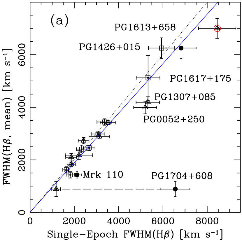
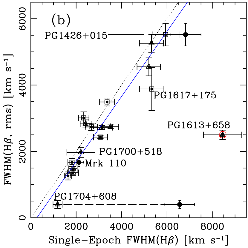
Figure 1: The distribution of FWHM(H $\beta$) in the mean (panel a) and rms (panel b) multi-epoch spectra and single-epoch FWHM(H $\beta$) of the PG quasars presented by Kaspi et al. (2000) and Mrk 110 and Mrk 335 (Wandel et al. 1999). The dotted line indicates a pure one-to-one relationship. The objects discussed in the text are labeled. The open squares denote Seyfert 1s while triangles show measurements for the quasars. The three solid circles show the measurements of Boroson & Green (1992) which are based on spectra with both Fe ii emission and the narrow core component subtracted. These FWHM measurements are not always representative of the BLR velocity dispersion needed for this study (see text). The solid line is the best fit BCES bisector regression line based on all the objects in the diagram except PG1613$+$658 (sample C; Table 3). The BCES (Y$|$X) and (X$|$Y) regressions are not plotted as they crowd the bisector. The single-epoch FWHM(H $\beta$) scatter around a one-to-one relationship with FWHM(H $\beta$, mean) to within 15% $-$ 20% variation and around a similar relationship with FWHM(H $\beta$, rms) to within 20% $-$ 25%. Note, the ordinate range is different in the two diagrams.

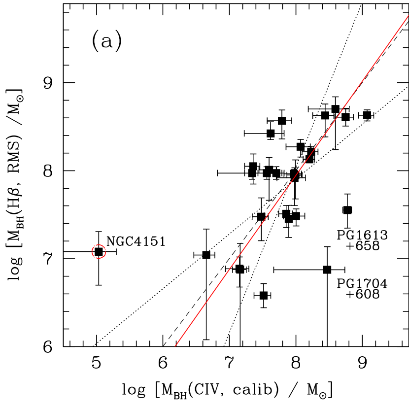
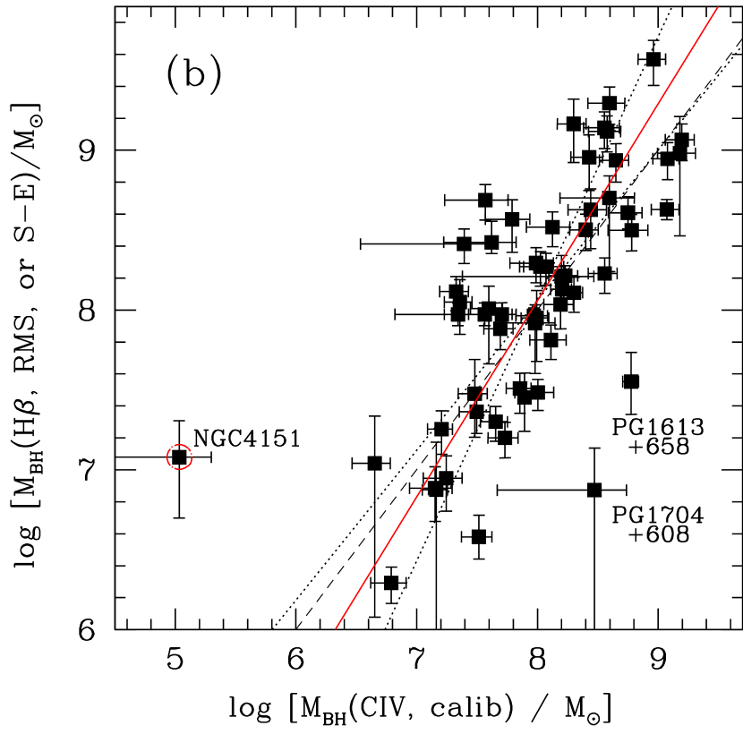
Figure 5: The central mass estimates based on the calibration of the UV spectral measurements are compared to central masses measured (and/or estimated; panel b) based on optical data. Dashed line: pure unity relationship. Dotted lines: BCES(Y$|$X) and BCES(X$|$Y) regression lines. Solid line: the BCES bisector. NGC 4151 was excluded from the regression analysis. (a) $M_{\rm BH,UV}$ estimates versus the established central masses, $M_{\rm BH}(\rm H\beta,rms)$ [UVrev sample only]. (b) $M_{\rm BH,UV}$ estimates are plotted for the full UV sample versus the “optical masses” described in Figure 8b. For both diagrams the mass relationships are consistent with a unity relationship within the uncertainties.

The objects labeled in Figure 8a (except PG1617$+$175) have BG92 FWHM(H $\beta$) measurements larger than FWHM(H $\beta$, mean) in excess of $\sim$20% variation and the typically expected measurement uncertainties. Are these deviating measurements easily understood? PG0052$+$250 and PG1307$+$085 are quite variable in the H $\beta$ line flux as indicated by the light curves of Kaspi et al. (2000) and so their deviating line widths are not unexpected. The “uncorrected” FWHM(H $\beta$) of Mrk 110 and PG1426$+$015 deviate from the BG92 measurements by more than 10%. Both objects have strong (spiky) narrow H $\beta$ components (see e.g., Fig. 1 by BG92) that were subtracted by BG92. This explains the larger BG92 widths. PG1613$+$658 behaves strangely. The mean H $\beta$ profile is broad but it varies most strongly in the narrow line core (see e.g., Figure 8b and Table 6 and Figure 5 of Kaspi et al. 2000). However, for this object the narrow component of neither the single-epoch profile nor the mean profile is a fair representation of the rms profile (Figure 8b). Therefore, this object will commonly be excluded from the analysis. To reiterate, for Mrk 110, PG1426$+$015, and PG1704$+$608 the single-epoch FWHMs based on the original, uncorrected data are used in the analysis instead of the BG92 values. For the remaining objects the single-epoch FWHM(H $\beta$) is consistent with FWHM(H $\beta$, mean) to within reasonable effects of line variability.

Figure 8b shows the single-epoch FWHM(H $\beta$) of BG92 with the corrections discussed above plotted versus the FWHM(H $\beta$, rms) [Wandel et al. 1999; Kaspi et al. 2000]. Most of the objects with single-epoch FWHM(H $\beta$) deviating from FWHM(H $\beta$, rms) by more than $+$15% were well within $\pm$15% from the FWHM(H $\beta$, mean) in Figure 8a. This may indicate that the variation in FWHM is typically a little larger than 15%, as is seen for NGC 5548, in these objects and mostly occur in the narrow line core. The main technical difference between the BG92 FWHM(H $\beta$) and the FWHM(H $\beta$, rms) is that the BG92 FWHM only reflects the width of the broad line component as both line widths are expected to be little affected by the presence of Fe ii emission. For objects with strong variation in the low-velocity gas the two FWHM measurements will therefore differ significantly as observed and discussed above. Of the two objects (PG1617$+$175 and PG1613$+$658) with single-epoch FWHM(H $\beta$) (and error) deviating by $\stackrel{{\scriptstyle\scriptscriptstyle>}}{{\scriptstyle{}_{\sim}}}$15% from FWHM(H $\beta$, rms), only PG1613$+$658 has such a significantly deviant BG92 FWHM(H $\beta$) that the offset cannot be ascribed to larger measurement uncertainties or stronger source variation than the $\pm$15% shown by NGC 5548.

It is worth noting for completeness that the differences in spectral resolution between the BG92 and the Kaspi et al. spectra do not contribute to the line width differences. The original BG92 spectra were degraded to the resolution of $\sim$10 Å of the Kaspi et al. spectra for this analysis. No significant FWHM differences were found.

4.1.3 Regression Analysis

Regression analyses were performed to statistically test how well the single-epoch FWHM(H $\beta$) represents the multi-epoch line widths. It is clear from Figure 8a that the objects with line widths below 4000 km s^-1 yield very consistent measurements in spite of their variability, while the broader lined objects have larger uncertainties from both measurements [recall, that a 10% measurement error was assumed for the single-epoch FWHM(H $\beta$)] and especially from intrinsic source variability; these objects have rather similar luminosities to the other objects in the sample, and so these differences are not likely luminosity-related. However, PG1613$+$658, PG1426$+$015, and PG1617$+$175 have the broadest mean H $\beta$ line and also strong, broad Fe ii emission (see BG92). This emphasizes the need for linear regression methods, which are more appropriate for the nature of these data. The regression analyses were therefore performed using the bivariate correlated errors and intrinsic scatter (hereafter BCES) algorithm (Akritas & Bershady 1996). When intercomparing the multi-epoch measurements with those of single-epoch spectra, intrinsic scatter and measurement errors are expected. The BCES algorithm is the most appropriate to use as it does not, as do many other linear regression methods, assume a perfect relationship between the variables if the measurement errors could be made insignificantly small. Merritt & Ferrarese (2001a) compare the BCES algorithm to other commonly used linear regression methods.

The uncertainties used in the regressions are the symmetric errors on the logarithms based on the positive linear errors. No significant differences were found when using the negative linear errors instead. These symmetric errors [= $(\log{e})\,(\sigma_{X}/X)$] were determined by propagating the linear errors to the logarithmic relationship.

The best fit to the FWHM(H $\beta$, mean) and FWHM(H $\beta$) distribution is shown in Table 3. It is based on sample B, that is, the PG quasars (Kaspi et al. 2000) and Mrk 110 and Mrk 335 (Wandel et al. 1999), excluding PG1351$+$640 as it has no H $\beta$ measurements available. The BCES regression is quite robust; bootstrapping simulations reproduce the theoretically expected results well (see e.g., Akritas & Bershady 1996). Also, there is little difference between the BCES(Y$|$X) [i.e., Y = f(X)] and BCES(X$|$Y) [i.e., X = g(Y)] regressions. The bisector bisects these two regressions and so the said small difference is reflected in the similar results obtained for the BCES(Y$|$X) and bisector regressions (both are listed in Table 3). These BCES regressions for all the data points in Figure 8a (sample B) are consistent with a unity relationship within 1.8$\sigma$. When the FWHM(H $\beta$, rms) measurements are considered (Fig. 8b) PG1613$+$658 is very much an outlier and it is excluded from the regressions to those data as it behaves in an obviously strange fashion (§ 4.1.2). For comparison with the results of that analysis, the regressions were repeated on the sample in Figure 8a excluding this object (sample C): the data now display a tighter relationship and the BCES regression is consistent with a unity relationship to within 1$\sigma$, with no regard to which is the independent variable (Table 3). Only the BCES bisector for sample C is shown in Figure 8a for visibility. The BCES bisector is also the most representative of the intrinsic relationship between the two line widths, because they are different measures of the same property.

In Figure 8b the bisector regression (solid line) for sample C shows consistency with a unity relationship to within 1 $\sigma$: FWHM(H $\beta$, rms) = (0.98$\pm$0.08)$\times$ single-epoch FWHM(H $\beta$) $-$ (265$\pm$227). Whether this relationship or a pure 1:1 relationship is used, the propagated effect on $\log$ $M_{\rm BH}$ is only of order $\sim$0.04 dex for a 4000 km s^-1 line width (and ranging between 0.07 and 0.03 dex for widths of 2000 km s^-1 and 6000 km s^-1, respectively) which is well within typical FWHM measurement uncertainties. So, assuming a 1:1 relationship is fair, as long as the single-epoch line width is measured as described in § 4.1.2.

4.1.4 Is the High-Velocity BLR Gas Optically Thin?

It is interesting to note that this comparison of FWHM(H $\beta$, rms) and single-epoch FWHM(H $\beta$) (with or without the Fe ii emission) shows that for the PG quasars the single-epoch FWHM(H $\beta$) is predominantly larger than the FWHM(H $\beta$, rms). If all the line flux, both at high and low velocity, in the profile is varying with similar amplitudes one would naïvely expect the rms profile to be consistently broader than any given single-epoch profile as the rms profile represents the responding amplitudes and the velocities of the responding gas. At the very least, the single-epoch width should scatter around FWHM(H $\beta$, rms). Yet the opposite is seen here. One may speculate whether this indicates that the broad line wings, which are often not represented in the rms line profiles, are mostly due to optically thin material, which does not respond to continuum variations as does optically thick gas? This is probably seen for He ii in NGC 4051 (Peterson et al. 2000). PG1704$+$608 and, especially, PG1613$+$658 were pointed out above as extreme cases showing broad average profiles, yet exhibit variability in the narrow line core only. Other objects showing similar behavior in their H $\beta$ line profiles are Mrk 590 (Ferland, Korista, & Peterson 1990) and Mrk 335 (Kassebaum et al. 1997). Similar behavior has been seen for both the Ly $\alpha$  and C iv line profiles in the higher luminosity quasars (e.g., O’Brien, Zheng, & Wilson 1989; Pérez, Penston, & Moles 1989; Gondhalekar 1990). Therefore, the presence of high-velocity, optically thin line emission is likely rather common in AGNs and quasars. Shields, Ferland, & Peterson (1995) discuss this issue and its possible importance. They further argue that the presence of such optically thin emission gas can explain some of the variability properties of Seyfert 1s.

To summarize § 4.1, statistically, the single-epoch H $\beta$ line width displays a unity relationship with both FWHM(H $\beta$, mean) and FWHM(H $\beta$, rms) to within 1$\sigma$. However, this is valid as long as the single-epoch FWHM(H $\beta$) is measured on H $\beta$ profiles, which includes the narrow component but for which especially strong (and blending) Fe ii emission is subtracted.

4.2 Luminosity Measurements

The optical continuum luminosities for the single-epoch spectra are gathered mostly from Neugebauer et al. (1987) supplemented with data from Schmidt & Green (1983) for Mrk 110 and Mrk 335, as described in § 3. In Figure 8 these $\lambda L_{\lambda}$(5100Å) measurements are compared to those determined by Wandel et al. (1999) and Kaspi et al. (2000) for the same sample of quasars discussed above in § 4.1 but including also PG1351$+$640 (i.e, sample A; Table 3); the luminosities are plotted with the same cosmology (H₀ = 75 ${\rm km~{}s^{-1}Mpc^{-1}}$, q₀ = 0.5, and $\Lambda$ = 0). The uncertainties listed by Kaspi et al., based on the rms in the continuum light curves, are also plotted. The single-epoch luminosity uncertainty reflects the propagated errors based on the measurement uncertainties as described in § 3.1. It is clear from Figure 8 that for most of the objects the luminosity measured by Neugebauer et al. is stronger.

Regression analyses show (Table 3) a best fit slope consistent with 1.0 and an intercept of zero to within the uncertainties. The various BCES results are rather robust and show little difference. Figure 8 indicates that most of the data points are scattered around a slope of one with a systematic offset of $\sim$0.1 dex, (i.e., $\sim$30%). This offset is equivalent to an offset in $\log$ M of 0.07 dex. As will be clear later, this is well within the uncertainties of the (calibrated) mass estimates and will thus not significantly affect the calibration of optical single-epoch mass estimates. Therefore the central mass estimate calibration is evaluated assuming no luminosity offset, i.e., no correction of either luminosity measurements is applied, but keeping the offset in mind. The $\sim$0.1 dex scatter in the luminosity measurements around the regression line is adopted as a representative uncertainty in using single-epoch luminosity measurements to measure the AGN mean luminosity (thus justifying the choice in § 3). A higher uncertainty may apply in practise, especially if (spectro-)photometric data are not used to determine the continuum luminosity.

For completeness it is noted that the luminosity offset is not caused by either (1) interpolation errors in the Neugebauer et al. data [tight spectral energy distributions; interpolation across neighboring pixels], (2) intrinsic source variability [possibly some contribution, but symmetric scatter around a one-to-one relationship would be expected], (3) aperture differences between the Kaspi et al. and Neugebauer et al. studies, or (4) different corrections for reddening or Galactic extinction. As for (3), both studies have apertures including equal amounts of host galaxy contributions, which afterall is only strong in a few objects (S. Kaspi 2001, private communication). However, the use of slightly different absolute flux calibration scales could be the origin of the systematic luminosity offset.

5 Calibration of Single-Epoch Mass Estimates: Optical Measurements

Having established that the single-epoch line widths and luminosities are statistically representative of the multi-epoch equivalent measurements, the “single-epoch central mass estimates” can be computed and further analyzed. The first step in the calibration of UV single-epoch measurements to estimate the central AGN/quasar mass is to compare and calibrate, if necessary, the single-epoch optical measurements to yield representative estimates of the central masses. This is done here using the sample of 18 objects with central mass determinations from reverberation mapping (Wandel et al. 1999; Kaspi et al. 2000) and H $\beta$ measurements.

Using the line widths and luminosities as discussed above the single-epoch mass estimates, $M_{\rm BH}(\rm H\beta)$, were computed for the 18 AGNs and quasars using equations (1) and (2). These masses are plotted in Figure 8 versus the masses determined from reverberation mapping studies. The masses quoted by Kaspi et al. (2000) are based on the average of the H $\beta$ and H $\alpha$ line widths. It is more appropriate to compare the single-epoch mass estimates with reverberation masses determined from the H $\beta$ line width only. The reasons are the following: (1) Kaspi et al. determined the BLR size, R_BLR, using data on both H $\alpha$ and H $\beta$ but found the same results using H $\beta$ alone, just with larger scatter, (2) The H $\alpha$ $\lambda$ 6563 profile is potentially contaminated by [N ii] $\lambda\lambda$ 6548, 6583 which will affect the FWHM(H $\alpha$) measurement, and, quite importantly, (3) the single-epoch mass estimates are based on H $\beta$ line widths only. Therefore, the reverberation masses were recomputed using equation (1) based on FWHM(H $\beta$), measured in the mean and rms spectra, respectively, and the directly measured BLR sizes, R_BLR, as listed in Tables 6 and 7 by Kaspi et al. (2000). These H $\beta$ based reverberation masses are listed in Table Determining Central Black Hole Masses in Distant Active Galaxies. along with the single-epoch mass estimates.

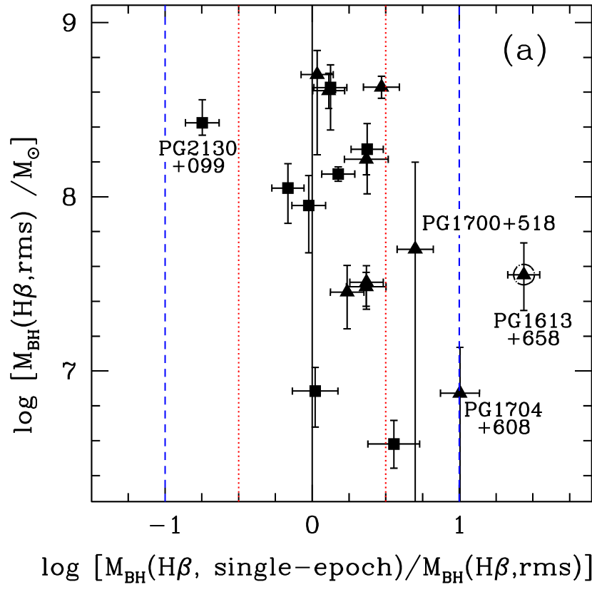
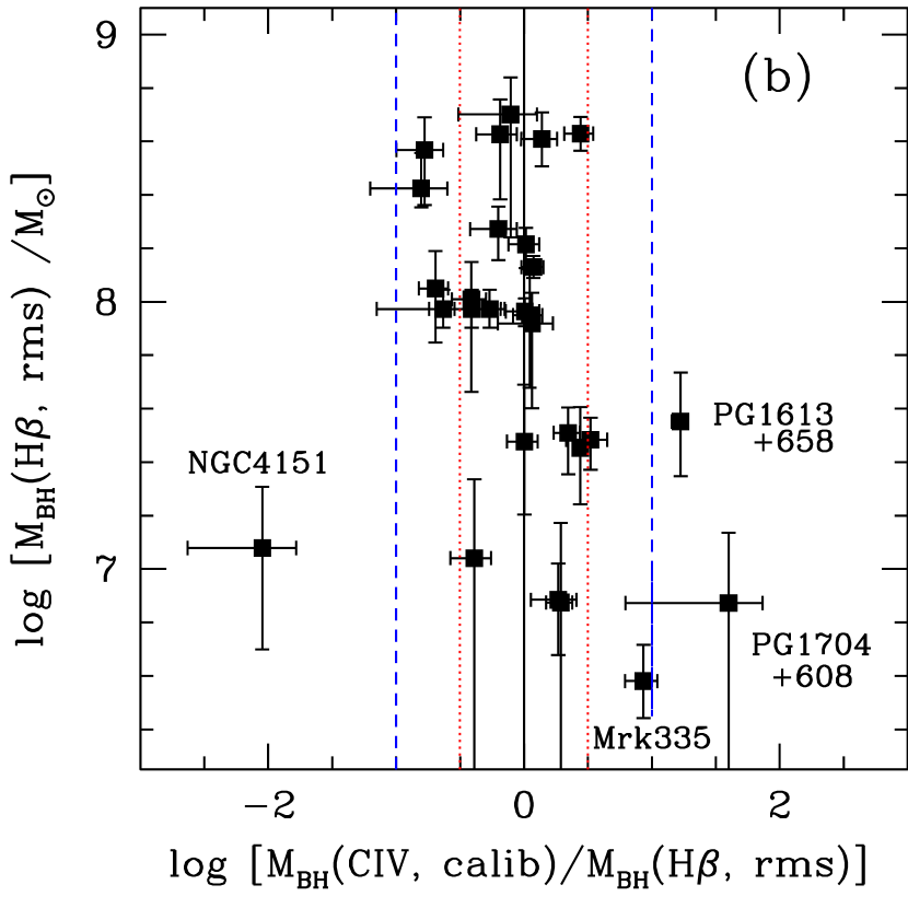
Figure 6: The established central masses, $M_{\rm BH}(\rm H\beta,rms)$, based on optical multi-epoch spectral measurements plotted versus the deviations of mass estimates based on calibrated single-epoch spectra. (a) Deviations of masses estimated from optical spectra, i.e., $M_{\rm BH}(\rm H\beta,S$-E)  divided by $M_{\rm BH}(\rm H\beta,rms)$. (b) Deviations in the masses based on UV spectral measurements, $M_{\rm BH,UV}$(C iv). The uncertainties in the abscissa are the (propagated) uncertainties in the single-epoch masses (i.e., not the mass deviation error). A strictly unity relationship is indicated by the solid line. Offsets of $\pm$0.5 dex ($\pm$1 dex) are indicated by the dotted (dashed) lines.

$M_{\rm BH}(\rm H\beta,rms)$ is plotted in Figure 8a with the single-epoch mass estimates for the 18 objects in sample B (see Table 3; PG 1351$+$064 has no H $\beta$ reverberation data). Similarly, $M_{\rm BH}(\rm H\beta,mean)$ is plotted in Figure 8b. The dashed line indicates a one to one relationship with no constant offset between the two mass measures. Some scatter is expected and observed and apart from the usual objects with deviating FWHM(H $\beta$) measurements (the outlying objects are labeled), most of the scatter is likely caused by the intrinsic scatter in the BLR size $-$ luminosity relationship (see Figure 6 by Kaspi et al. 2000). This scatter is the cause of PG2130$+$099 being an outlier in these diagrams. Disregarding PG1613$+$658, which all along has not behaved well, and for a moment the two objects with rather larger uncertainties in their mass estimates, PG1700$+$518 and PG1704$+$608, the scatter in the $M_{\rm BH}(\rm H\beta,rms)$$-$ $M_{\rm BH}$(H $\beta$, single-epoch) relationship is afterall comparable to the uncertainties in the mass estimates. The best fit regression slopes are also plotted in Figure 8. The solid lines are the BCES bisectors when omitting the encircled object (PG1613$+$658). The dotted line is the BCES bisector to all the data points in each diagram.

The results of the linear regressions and the detailed fitting parameters are listed in Table 4. The issue of establishing the intrinsic relationship between these two mass estimates (single-epoch versus multi-epoch) is very similar to that of the most accurate representation of the intrinsic relationship between, say, the black hole mass, $M_{\rm BH}$, and the stellar velocity dispersion in the host galaxy (e.g., Gebhardt et al. 2000a; Ferrarese & Merritt 2000; Merritt & Ferrarese 2001a). In both cases the relationship is sought between two variables with both measurement uncertainties and intrinsic scatter. Therefore, for the calibration of the single-epoch mass estimates, the use of the BCES linear regression algorithm is very important.

The mass comparison of most importance for the calibration is that with $M_{\rm BH}(\rm H\beta,rms)$ (see § 2). Since both the single-epoch mass estimate and the reverberation mass are (different) measures of the same property, the BCES bisector is the most appropriate regression to use. It is apparent from Table 4, however, that using either of the BCES (Y$|$X) and bisector regressions yields the same basic results within the uncertainties. Namely, there is a pure unity relationship between $M_{\rm BH}$(H $\beta$, single-epoch), hereafter $M_{\rm BH}(\rm H\beta,S$-E), and $M_{\rm BH}(\rm H\beta,rms)$ within $\stackrel{{\scriptstyle\scriptscriptstyle<}}{{\scriptstyle{}_{\sim}}}$0.25$\sigma$, for BCES(Y$|$X):

$$\log\,{M}_{\rm BH}{\rm(H_{\beta},rms)} = (0.97\pm 0.13)\times\log\,M_{\rm BH}(\rm H_{\beta},S-E)$$ (3)

$$+(0.05\pm 1.08)$$

and for the BCES bisector:

$$\log\,{M}_{\rm BH}{\rm(H_{\beta},rms)} = (1.03\pm 0.14)\times\log\,M_{\rm BH}(\rm H_{\beta},S-E)$$ (4)

$$-(0.49\pm 1.17)$$

The uncertainties used in the regression are, again, the symmetric errors on the logarithms based on the positive linear errors [i.e., = $(\log{e})\,(\sigma_{X}/X)$; § 4].

For completeness the single-epoch mass estimates are also compared with the reverberation masses based on the FWHM(H $\beta$, mean) measured in the multi-epoch spectra (Fig. 8b). The outliers (labeled) are again the ‘usual suspects’ (§ 4.1.2 and above). Again, there is a unity relationship, but with less scatter (Table 4). This is expected as the single-epoch FWHM(H $\beta$) also show less scatter with FWHM(H $\beta$, mean) than with FWHM(H $\beta$, rms) [§ 4.1]. When comparing the single-epoch masses to the masses computed by Kaspi et al. (i.e., based on both H $\alpha$ and H $\beta$) larger scatter and poorer fits are obtained. This is expected, as explained, and stresses the need to use the reverberation masses based on H $\beta$ measurements only.

In conclusion, the calibration of single-epoch “optical” mass estimates to the multi-epoch reverberation masses is, with the current uncertainties, a one-to-one relationship with no significant zero-point offset and no apparent reasons to further correct $M_{\rm BH}(\rm H\beta,S$-E). Note, however, that this assumes the line widths are measured as described in § 4.1. The performance of the optical single-epoch mass calibration and how it compares to the UV single-epoch mass calibration, derived below, are discussed in § 7.

6 Calibration of Single-Epoch Mass Estimates: UV Measurements

In this section a calibration is determined of UV spectral measurements to reflect reasonable estimates of the central masses. Two subsets of data are used here. The primary sample (UVrev) is the collection of 26 AGNs and quasars with central mass determinations from reverberation mapping (Wandel et al. 1999; Kaspi et al. 2000) for which C iv line widths, FWHM(C iv), and UV continuum luminosities, $\lambda L_{\lambda}$(1350Å), are available in the literature. For this sample the UV measurements will be directly compared with the available reverberation mass determinations, $M_{\rm BH}(\rm H\beta,rms)$. By using this sample the UV calibration is based on fewer assumptions than if additional objects were included. This is because the single-epoch UV mass estimates are compared to independently measured central masses and not to masses estimated based on, for example, optical measurements.

Nevertheless, it is instructive to compare the results of the UVrev sample with those of a larger sample (named “sample UV” in the following). The latter sample consists of sample UVrev and 30 other PG quasars for which FWHM(C iv) and UV continuum luminosities are likewise readily available (Table Determining Central Black Hole Masses in Distant Active Galaxies.). For these additional quasars, no reverberation masses are available but the central masses are here determined from the calibration of single-epoch optical measurements, derived in § 5. It is clear that since these masses are estimates they are expected to introduce some uncertainty, which is why they only serve to provide a comparison and an additional check on the performance of the calibrations. However, as discussed later, this uncertainty appears to be within the scatter intrinsic to the reverberation masses, which indicates that the calibrations are relatively reliable.

In § 4.1 it was necessary to remeasure the single-epoch FWHM(H $\beta$) on the original, uncorrected data (from BG92) to ensure that the subtraction of the narrow emission component by BG92 would not affect the line width measurement adversely. This was important for the use of FWHM(H $\beta$) to estimate the central mass, as discussed there. Similarly, the single-epoch FWHM(H $\beta$)’s were remeasured for the subset of 30 PG quasars, studied by BG92, which are used here to extend the primary sample of reverberation mapped AGNs (UVrev). And similar to the approach adopted in § 4.1 each remeasured single-epoch FWHM(H $\beta$) was compared to the BG92 measurement and corrected based on the same considerations. Similar to the UVrev objects the optical single-epoch continuum luminosities, $\lambda L_{\lambda}$(5100Å), were determined from the tabulated spectral energy distributions of Neugebauer et al. (1987) or the photometry of Schmidt & Green (1983). The ‘optical mass estimates’ were then determined from equation (1) and (2), as justified in § 5. The adopted optical measurements, FWHM(H $\beta$) and $\lambda L_{\lambda}$(5100Å), and the single-epoch mass estimates, $M_{\rm BH}(\rm H\beta)$, are listed in Table Determining Central Black Hole Masses in Distant Active Galaxies..

The calibration of the UV measurements to reflect the central mass is described in the following. First, the mass is expected to depend on FWHM²(C iv). Anything else would not be physical (according to the virial theorem). Second, one can assume that the continuum luminosity enters to the power 0.7 as was established for the optical measurements (Kaspi et al. 2000; see also Appendix A for a discussion thereof), since the continuum luminosities at 5100 Å and 1350 Å are generally expected to be related (via the assumed power-law relationship, $L_{\nu}\propto\nu^{-\alpha}$). The validity of this latter assumption can be tested by computing the BCES regressions between the already established masses and what can be called the normalized UV mass, $nM_{\rm BH,UV}$= FWHM²(C iv) [$\lambda L_{\lambda}$(1350Å)]^0.7. The question is thus whether $nM_{\rm BH,UV}$ is related to $M_{\rm BH}$ to the first power and what is the global scaling factor? The regression results are presented in Table 5 for the two basic samples, namely sample UVrev and sample UV, and are discussed below. In this case where the relationship between $nM_{\rm BH,UV}$ and the reverberation mass, $M_{\rm BH}(\rm H\beta,rms)$, will be used to calibrate other data it is very important to choose the most appropriate statistical method to characterize the intrinsic relationship between these two variables. Different regressions [e.g., (Y$|$X), bisector, and orthogonal regressions] yields statistically different results as they measure different moments of the data (e.g., Isobe et al. 1990; Feigelson & Babu 1992). Which is then the most appropriate BCES regression (moment) to use for the calibration? This is not clear even from a statistical point of view. Therefore, the following approach is adopted. First, BCES regression analyses are performed to test whether the relationship between $\log$ $nM_{\rm BH,UV}$ and $\log$ $M_{\rm BH}(\rm H\beta,rms)$ are indeed consistent with a slope of 1.0 to within the uncertainties. This justifies the assumption that $M_{\rm BH,UV}$ = constant $\times$ FWHM²(C iv) [$\lambda L_{\lambda}$(1350Å)]^0.7 as discussed above and also justifies the next step. Once this unity slope is established the problem reduces to the simple relationship with only one degree of freedom: $y~{}=~{}x~{}+~{}a$ or $a~{}=~{}y~{}-~{}x$, where both $y$ (= log $M_{\rm BH}(\rm H\beta,rms)$) and $x$ (= log $nM_{\rm BH,UV}$) have uncertainties. The constant zero point offset, $a$, can therefore be determined as the weighted mean of  ‘$~{}y~{}-~{}x~{}$’  determined for the individual objects. This approach limits the introduction of unnecessary systematic errors that would occur if both the slope and intercept are free parameters. Once $a$ is determined, it can be tested that the calibrated UV estimates, $M_{\rm BH,UV}$= $nM_{\rm BH,UV}$$\times 10^{a}$, are indeed related to the established central masses, $M_{\rm BH}(\rm H\beta,rms)$, in a pure one-to-one relationship (i.e., a BCES bisector slope of unity and no zero-point offset).

Figure 8 displays the distribution of $nM_{\rm BH,UV}$ and $M_{\rm BH}(\rm H\beta,rms)$ for the UVrev sample (panel a) and for the full UV sample (panel b). The dotted line is the BCES bisector to all the displayed data points, while the dashed line represents the bisector when NGC 4151 is excluded (see below). The solid lines are the BCES (Y$|$X) and (X$|$Y) regressions to the latter data. For the UVrev sample alone there is a larger difference between the bisector and BCES(Y$|$X) slopes (Fig. 8a; Table 5) than for the UV sample (Fig. 8b), indicating the relatively larger scatter in the UVrev sample. [This is expected, however, as the 30 additional PG quasars have smaller intrinsic scatter in their optical mass estimates, $M_{\rm BH}$(H $\beta$), owing to their origin in the mass relationship in eqns. (1) and (2)]. As is also clear from these figures, NGC 4151 has large uncertainties and is very much an outlier. Excluding this data point clearly has a significant effect on the slope in both cases (samples UVrev,b and UVb in Table 5). The BCES bisector for sample UVrev,b then shows a slope of 1.0 to within 0.3$\sigma$. The BCES (Y$|$X) regression is consistent with unity to within $<2.5\sigma$; the uncertainty is somewhat large due to the intrinsic scatter in this sample. Note that, excluding also PG1704$+$608 and/or PG1613$+$658 does not significantly change the regressions. When the 30 additional PG quasars are included the statistical significance increases and also provides a larger mass range. In effect this allows the relationship to be better constrained (e.g., Fig. 8b). As seen in Table 5 for sample UV the (Y$|$X) slope is now increased to 0.7 and is improving further when NGC 4151 is excluded (sample UVb). In this case both the BCES (Y$|$X) and bisector slopes are consistent with a unity relationship to within at most $\sim 2\sigma$, which is acceptable. That is, both the UVrev,b and UVb samples show similar relationships in the mass comparisons, although with different scatter and uncertainties.

The fact that NGC 4151 significantly changes the regression results argues that it should not be included in the calibration for the same reason that PG1613$+$658 was excluded from the optical calibration: it likely behaves differently than the bulk of the AGNs and quasars, and it is thus inappropriate to apply a calibration to large samples of AGNs that are based on and significantly affected by (possibly) strangely behaving objects.

Since indeed $\log$ $nM_{\rm BH,UV}$ and $\log$ $M_{\rm BH}(\rm H\beta,rms)$ are related with slope $\equiv$ 1.0, the intercept can be determined as the weighted mean of the individual mass differences; their uncertainties are propagated from the individual errors on $nM_{\rm BH,UV}$ and $M_{\rm BH}(\rm H\beta,rms)$. For sample UVrev,b the weighted mean is

$$<\log\,{M_{\rm BH}}{\rm(H_{\beta},rms)}-\log\,nM_{\rm BH,UV}>~{}=~{}6.2\pm 0.03$$ (5)

where the uncertainty is the precision based on the propagated errors. The sample standard deviation is 0.45 showing the presence of real intrinsic scatter, as expected (e.g., Fig. 8). Excluding the other outliers (PG1613$+$658 and PG1704$+$608) does not significantly change the results. The weighted mean computed for the full UVb sample is the same, showing a difference only on the second significant digit (likewise for the precision and the sample standard deviation). The fact that UVrev,b and UVb show very similar results confirms again that the optical single-epoch mass estimate is a fair representation of the reverberation masses (based on the current data).

How do the calibrated UV estimates, $M_{\rm BH,UV}$= $nM_{\rm BH,UV}$$\times 10^{6.2}$, relate to the established central masses, $M_{\rm BH}(\rm H\beta,rms)$? In Figure 8 $M_{\rm BH,UV}$ are plotted versus $M_{\rm BH}(\rm H\beta,rms)$ for the UVrev sample (panel a) and versus $M_{\rm BH}(\rm H\beta,rms)$ or $M_{\rm BH}(\rm H\beta,S$-E) for the full UV sample (panel b). The regression results (excluding NGC 4151; Table 5) are also shown. The BCES (Y$|$X), (X$|$Y) (dotted lines) and bisector (solid line) regressions, and a pure 1:1 relationship (dashed line) are also shown. The most important comparison here is that with the independently established reverberation masses in Figure 8a. The UV sample is shown in Figure 8b for completeness. The BCES bisector fit to the objects in the UVrev,b sample (excluding NGC 4151) yields the following result:

$$\log\,M_{\rm BH}{\rm(H_{\beta},rms)}=$$ (6)

$$(1.07\pm 0.14)\times\log\,M_{\rm BH,UV}-0.61\pm 1.11$$

The bisector is consistent with a unity relationship to within 0.5$\sigma$, thereby indicating that the UV calibration is robust.

When the additional 30 PG quasars are included (Fig. 8b) with single-epoch optical mass estimates a slightly steeper bisector is found. However, this sample is also consistent with a unity relationship in this calibration. In this case, it is so to within $\sim 2\sigma$ and is still acceptable. Although the two samples have different intrinsic scatter it is comforting to see that they yield consistent results, as pointed out earlier.

In conclusion, the best calibration of the UV measurements appear to be

$$\log\,M_{\rm BH}{\rm(H_{\beta},rms~{}or~{}SE)}=$$ (7)

$$\log\,\left[\left({\rm\frac{FWHM(C\,IV)}{1000~{}km~{}s^{-1}}}\right)^{2}~{}\left(\frac{\lambda L_{\lambda}\rm(1350\AA)}{10^{44}\rm~{}ergs~{}s^{-1}}\right)^{0.7}\right]$$

$$\mbox{}+6.2\pm 0.03~{}~{}(\pm 0.45)$$

The last parenthesis contains the sample standard deviation of the weighted mean, which shows the intrinsic scatter in the sample. As opposed to the uncertainty or precision of 0.03 on this weighted mean the standard deviation is probably more representative of the uncertainty in the offset for this (UVb) sample. It is also specific for the result obtained in the logarithmic representation and makes little sense when linearized. Therefore, no uncertainties are listed for the linear scaling factor below. In linear representation, the calibration is:

$$M_{\rm BH,UV}=$$ (8)

$$1.6\,\times 10^{6}\left(\rm\frac{FWHM(C\,IV)}{1000~{}km~{}s^{-1}}\right)^{2}\,\left(\frac{\lambda L_{\lambda}\rm(1350\AA)}{10^{44}\rm~{}ergs~{}s^{-1}}\right)^{0.7}$$

The mass calibrations rely strongly on the size $-$ luminosity relationship and its intrinsic scatter dominate the uncertainties in the mass estimates. Such scatter is naturally expected given the nature of the objects and the nature of the obtained BLR sizes based on continuum variability (e.g., Netzer & Peterson 1997). Once a larger sample of AGNs with reverberation mapping masses is available, the $R_{\rm BLR}-L$ relationship should be updated. Because it matters how this relationship is established, a slightly modified approach to that adopted by Kaspi et al. (2000) is advocated in Appendix A. Note that, the modified approach does not significantly affect the current $R_{\rm BLR}-L$ relationship.

7 How Reliable Are the Calibrations?

It is of keen interest to ask how much of an error we typically will make on the mass estimate using the virial mass-luminosity-FWHM relationship [eqn (1) and (2)] when instead of the FWHM(H $\beta$,rms) and the mean monochromatic luminosity, $\lambda L_{\lambda}$, we use FWHM and $\lambda L_{\lambda}$ measurements of a single-epoch spectrum, which is in fact a ‘snap-shot’ spectrum at any random given time? Clearly, this is only an approximation with the caveat that the estimated central mass may be off by a large factor. But what is the probability for that? In the following, the approximate uncertainties are briefly evaluated, assuming that the sample of 26 (18) nearby AGNs and quasars studied using reverberation mapping techniques is representative for the UV (optical) calibration uncertainties.

In Figure 8 the reverberation masses, $M_{\rm BH}(\rm H\beta,rms)$, are plotted against the deviation in the optical (panel a) and UV (panel b) mass estimates from this established mass. Offsets of 0.5 dex and 1.0 dex from a perfect one-to-one relationship are indicated. The probabilities of estimating the mass with a certain accuracy are summarized below and in Table 6. For the optical single-epoch mass estimates Figure 8a shows 17 objects out of the 18 available to have single-epoch mass estimates deviating by $\stackrel{{\scriptstyle\scriptscriptstyle<}}{{\scriptstyle{}_{\sim}}}$1.0 dex. That is, there is a probability of $\sim$95% of getting the mass accurate to within an order of magnitude using single-epoch optical spectrophotometry. Similarly, there is a $\sim$90% probability of getting the mass accurate to within a factor of 6, and as much as a $\sim$80% probability of $M_{\rm BH}(\rm H\beta,S$-E) being “correct” to within a factor of 3 (Table 6). In other words, the 1 $\sigma$ uncertainty in $M_{\rm BH}(\rm H\beta,S$-E) is a factor of $\stackrel{{\scriptstyle\scriptscriptstyle<}}{{\scriptstyle{}_{\sim}}}$2.5.

Three of the 26 objects in Figure 8b deviate in $M_{\rm BH,UV}$(C iv, S-E) by more than 1 dex from the reverberation mass, $M_{\rm BH}(\rm H\beta,rms)$. There is, thus, a $\sim$90% probability of obtaining a central mass, accurate to within an order of magnitude, using single-epoch UV spectral measurements. As listed in Table 6 and illustrated in Figure 8b, the probability of obtaining a mass to within a factor of 3 is as high as 70% (1 $\sigma$ error), and there is an even higher chance (85%) of the mass being within a factor of 6 based on the UV calibration presented here.

The estimated uncertainty intrinsic to the reverberation technique is less than a factor of 2. Therefore, it is expected that the mass estimates based on the current optical and UV calibrations are not all reliable within as little as a factor of 3. Yet it is reassuring that this relatively high accuracy can be achieved in a high 70% $-$ 80% of the objects (UV and optical calibrations, respectively).

Figure 8 shows a tendency of the lower-mass objects to be overestimated in the single-epoch masses for both the optical and UV calibrations. This may be an “artifact” of the objects with very narrow and spiky line profiles. This is demonstrated in Figure 8 where the same mass deviations are plotted against FWHM(H $\beta$, rms) – the width of the variable H $\beta$ profile (left panel) — and against FWHM(C iv, S-E) – the single-epoch C iv widths (right panel) — since a C iv rms width is only known for very few of the objects. Clearly, the most narrow-lined objects or those varying strongly in their narrow line core tend to be overestimated in their central masses. This is most pronounced for the optical mass estimates; note, it is inherit in the calibration process that the UV masses will scatter almost symmetrically about $M_{\rm BH}(\rm H\beta,rms)$.

The good fortune is that the UV calibration appears to perform better for the higher mass and higher luminosity quasars, i.e., for FWHM(C iv) $>$ 4000 km s^-1 and/or $M_{\rm BH}$ $\stackrel{{\scriptstyle\scriptscriptstyle>}}{{\scriptstyle{}_{\sim}}}5\times 10^{7}$$M_{\odot}$. This is very comforting as its primary application will be to samples of high-redshift quasars, which are known to be of higher luminosity and are expected to occupy the higher end of the black-hole mass range observed ($\sim 4\times 10^{7}-1\times 10^{9}$$M_{\odot}$; see also e.g.  Laor 2000; Ho 2001). If the sample of PG quasars are representative most if not all quasars can thus have their central masses estimated to within a factor of $\sim$5 or less (Figures 8 and 8).

Since the mass estimates are very sensitive to the line width it is important that the signal-to-noise in the measured spectra is sufficiently high that the FWHM is measured relatively accurately (e.g., with a reliable uncertainty of 10% or less). This is worth keeping in mind, especially when studying distant, faint quasars. It still applies, however, that there is a 85% (90%) probability that the central masses can be estimated to within a factor of 6 based on UV (optical) data. This is reliable enough for many statistical applications.

In conclusion, both the optical and UV single-epoch mass estimates indicate approximately similar probabilities of obtaining reliable mass estimates with the optical calibration performing slightly better in general. The 1 $\sigma$ uncertainty is a factor of 3 or better. The UV calibration performs very well for the higher mass, broader lined objects where practically all the mass estimates are within a factor of $\sim$5 or less of the reverberation mapping masses.

8 Summary and Conclusions

Virial estimates of central black hole masses based on either optical or UV single-epoch spectrophotometry are calibrated to recently measured masses of nearby AGNs and quasars using reverberation mapping techniques. Single-epoch spectral measurements allow the central masses of distant AGNs and quasars to be easily estimated. This is important when more direct mass measurement techniques cannot easily be applied; moreover, this method allows estimates of masses of large samples of AGNs in a short time span. The following conclusions are reached:

• The current data show that the above-mentioned mass estimates are best made as follows:

  • The signal-to-noise in the single-epoch spectra is high enough that the FWHM can be measured reliably to an accuracy of 10% or better.

  • The FWHM is measured on a H $\beta$ or C iv emission line profile corrected for strong, contaminating Fe ii emission. But, for higher luminosity sources (i.e., quasars), narrow-line subtraction should not be attempted.

  • The continuum luminosity measured at 5100Å or 1350Å is used to estimate the relevant distance of the H $\beta$ or C iv emission line gas, respectively, using the empirical $R_{\rm BLR}-L$ relationship (Kaspi et al. 2000).

• The 1 $\sigma$ uncertainty in the optical and UV calibrations are a factor of 2.5 and 3, respectively.

  • Mass estimates based on single-epoch optical spectra are statistically consistent with the reverberation masses to within the uncertainties for the current database. The ‘optical single-epoch mass estimate’ measure the reverberation masses to within factors of 3, 6, and 10 with probabilities of 80%, 90%, and 95%, respectively.

  • The ‘UV single-epoch mass estimate’ measure the reverberation masses to within factors of 3, 6, and 10 with probabilities of 70%, 85%, and 90%, respectively.

• The most deviating mass estimates are found for the lower mass, more narrow-lined and/or lower luminosity AGNs. For quasars with FWHM(C iv) $>$4000 km s^-1 essentially all masses here are accurate to within a factor of 3 to $\sim$5. Thus these calibrations seem to perform very well where they are most needed, that is at high redshift for higher luminosity, more massive, quasars.

• The currently obtainable accuracy and associated probabilities are quite fair given the intrinsic uncertainty (factor less than 2) in the reverberation masses. An increase in the accuracy of the calibrations require a smaller scatter in the BLR size $-$ luminosity relationship. A decrease in the measurement uncertainties of the BLR size from reverberation studies will help. However, it is equally important that the BLR size be determined for as large a sample of AGNs and quasars as possible (and larger than the current sample of 34 objects) spanning a range of AGN properties.

The distribution of FWHM(H $\beta$) in the mean (panel a) and rms (panel b) multi-epoch spectra and single-epoch FWHM(H $\beta$) of the PG quasars presented by Kaspi et al. (2000) and Mrk 110 and Mrk 335 (Wandel et al. 1999). The dotted line indicates a pure one-to-one relationship. The objects discussed in the text are labeled. The open squares denote Seyfert 1s while triangles show measurements for the quasars. The three solid circles show the measurements of Boroson & Green (1992) which are based on spectra with both Fe ii emission and the narrow core component subtracted. These FWHM measurements are not always representative of the BLR velocity dispersion needed for this study (see text). The solid line is the best fit BCES bisector regression line based on all the objects in the diagram except PG1613$+$658 (sample C; Table 3). The BCES (Y$|$X) and (X$|$Y) regressions are not plotted as they crowd the bisector. The single-epoch FWHM(H $\beta$) scatter around a one-to-one relationship with FWHM(H $\beta$, mean) to within 15% $-$ 20% variation and around a similar relationship with FWHM(H $\beta$, rms) to within 20% $-$ 25%. Note, the ordinate range is different in the two diagrams.

(a) The distribution of the mean $\lambda L_{\lambda}$(5100Å) multi-epoch measurements (Wandel et al. 1999; Kaspi et al. 2000) based on monitoring data with respect to the single-epoch $\lambda L_{\lambda}$(5100Å) measurements of Neugebauer et al. (1987) and Schmidt & Green (1983). The errors in the mean $\lambda L_{\lambda}$(5100Å) are the rms around this mean. The errors in the single-epoch $\lambda L_{\lambda}$(5100Å) are propagated errors (see text). The short-dashed line (centrally positioned) denotes a one-to-one relationship. The dotted and long-dashed lines represent $\pm$30% and $\pm$60% luminosity variations, respectively (see text). (b) The best fit regression lines are shown for the BCES bisector (solid line). The BCES (Y$|$X) and (X$|$Y) regression lines would crowd the bisector, if plotted. All these BCES regression fits are consistent with a slope of 1.0. The single-epoch luminosities are offset by $+$0.138 dex at $\lambda L_{\lambda}$(5100Å) $\approx$ 44.8 ergs s^-1, the mid-range luminosity, based on the BCES bisector.

The reverberation masses derived from the rms (panel a) and mean (panel b) spectra plotted versus the single-epoch mass estimates based on optical spectral measurements. Triangles denote quasars, while squares denote Seyfert 1s. The dashed line indicates a unity relationship. The dotted line is a BCES bisector regression line to all the PG quasars with H $\beta$ measurements (shown), while the solid line is the BCES bisector when PG1613 is excluded (see text). As expected, $M_{\rm BH}(\rm H\beta,S$-E) show less scatter with $M_{\rm BH}(\rm H\beta,mean)$. Both relationships are consistent with a one-to-one relationship to within the errors.

Established and estimated central masses based on optical data plotted versus the UV measurements. This distribution is the basis of the calibration of the UV measurements. The “optical masses” (ordinate) in panel (a) consist of the reverberation masses, $M_{\rm BH}(\rm H\beta,rms)$, (filled, circled squares) derived from the rms spectrum and based on H $\beta$ only. In panel (b) these masses are supplemented with the single-epoch mass estimates, $M_{\rm BH}(\rm H\beta,S$-E), (filled squares) for the 30 PG quasars with no reverberation mapping masses. Dotted lines: BCES bisector regression lines to all the objects in each diagram. Solid lines: BCES(Y$|$X) and (X$|$Y) regressions to all the objects except NGC 4151 (see text). Dashed lines: the BCES bisector for all objects excluding NGC 4151.

The central mass estimates based on the calibration of the UV spectral measurements are compared to central masses measured (and/or estimated; panel b) based on optical data. Dashed line: pure unity relationship. Dotted lines: BCES(Y$|$X) and BCES(X$|$Y) regression lines. Solid line: the BCES bisector. NGC 4151 was excluded from the regression analysis. (a) $M_{\rm BH,UV}$ estimates versus the established central masses, $M_{\rm BH}(\rm H\beta,rms)$ [UVrev sample only]. (b) $M_{\rm BH,UV}$ estimates are plotted for the full UV sample versus the “optical masses” described in Figure 8b. For both diagrams the mass relationships are consistent with a unity relationship within the uncertainties.

The established central masses, $M_{\rm BH}(\rm H\beta,rms)$, based on optical multi-epoch spectral measurements plotted versus the deviations of mass estimates based on calibrated single-epoch spectra. (a) Deviations of masses estimated from optical spectra, i.e., $M_{\rm BH}(\rm H\beta,S$-E)  divided by $M_{\rm BH}(\rm H\beta,rms)$. (b) Deviations in the masses based on UV spectral measurements, $M_{\rm BH,UV}$(C iv). The uncertainties in the abscissa are the (propagated) uncertainties in the single-epoch masses (i.e., not the mass deviation error). A strictly unity relationship is indicated by the solid line. Offsets of $\pm$0.5 dex ($\pm$1 dex) are indicated by the dotted (dashed) lines.

The mass deviations from Figure 8 plotted here versus the H $\beta$ and C iv line widths. The optical mass deviations are plotted against FWHM(H $\beta$, rms), the width of the rms profile (i.e., the variable part), in (a) and versus the single-epoch FWHM(C iv) in (b). Lines and symbols are as in Figure 8. Notice that the larger mass discrepancies tend to occur for the most narrow lined objects in both cases (or those with the strongest variability occurring in the narrow line core: PG1613$+$658 and PG1704$+$608).

Appendix A The BLR Size $-$ Luminosity Relationship Revisited

The aim of this section is twofold, namely (1) to demonstrate the importance of using regression analysis that is appropriate for the nature of the data set, and (2) to advocate a careful assessment of the object sample on which important calibrations, such as the $R_{\rm BLR}-L$ relationship, are based. While this approach yields an $R_{\rm BLR}-L$ relationship consistent with equation (2) for the current object sample and data base, it is expected to become important once more data are available, allowing better constraints to be placed on this relationship.

Kaspi et al. (2000) established the empirical relationship [equation (2)] between the BLR size as measured by reverberation mapping and the intrinsic continuum luminosity of the objects using linear regression techniques that take errors in both variables into account. However, as the relationship is sought between two variables that have both measurement uncertainties and intrinsic scatter, it is important to use the bivariate correlated errors and intrinsic scatter (BCES) algorithm (Akritas & Bershady 1996) to establish the best size $-$ luminosity relationship. The results of applying this more appropriate linear regression analysis is shown in Table A. The regression was done between $\log\,R_{\rm BLR}$ and $\log$[$\lambda L_{\lambda}$(5100Å)/10${}^{44}\rm~{}ergs~{}s^{-1}$] to allow a linear regression. Although $R_{\rm BLR}$ is physically speaking a function of the luminosity and thus the BCES(Y$|$X) is the appropriate regression to use, the BCES(X$|$Y) and bisector regression results are also listed for completeness. The more accurate BLR size of 5.9${}^{+3.0}_{-2.0}$ for NGC 4051 (Peterson et al. 2000) is used here instead of that listed by Kaspi et al. (2000), but is not the cause of the differences discussed below.

When intrinsic scatter is accounted for the luminosity clearly enters with a power different from 0.7 (Table A), the luminosity power established by Kaspi et al. The linear equivalents of the $\log-\log$ BCES regressions are for the sample including NGC 4051:

$$R_{\rm BLR}=(20.9\pm 4.7)\left[\frac{\lambda L_{\lambda}\rm(5100\AA)}{10^{44}\rm~{}ergs~{}s^{-1}}\right]^{(0.38\pm 0.14)}$$ (A1)

for the Seyfert 1s alone, and for the PG quasars alone:

$$R_{\rm BLR}=(41.8\pm 8.3)\left[\frac{\lambda L_{\lambda}\rm(5100\AA)}{10^{44}\rm~{}ergs~{}s^{-1}}\right]^{(0.52\pm 0.09)}$$ (A2)

The linear relationship for the combined sample is:

$$R_{\rm BLR}=(32.4\pm 4.7)\left[\frac{\lambda L_{\lambda}\rm(5100\AA)}{10^{44}\rm~{}ergs~{}s^{-1}}\right]^{(0.58\pm 0.09)}$$ (A3)

The uncertainties used in the regression are the symmetric errors on the logarithms based on the positive linear errors. The errors on the proportionality factor are the linearized errors of the errors on $\log R_{\rm BLR}$, listed for comparison with eqn. 2.

When the intrinsic scatter in the data is accounted for the luminosity dependence of the BLR size weakens and the uncertainties are increased [eqn. (A3)]. However, these larger uncertainties are perhaps more representative than those returned by a weighted regression alone (eqn. 2). Note that the slopes of the individual samples [eqn. (A1) and (A2)] are consistent within their errors.

Peterson et al. (2000) find that NGC 4051 is peculiar as it has a larger BLR size for its luminosity than the other objects, deviating by almost 3$\sigma$. Excluding this object they find a luminosity dependence to the power 0.6 using a variance weighted regression algorithm similar to Kaspi et al., who included all objects in their regression. When NGC 4051 is excluded the BCES linear regressions change as follows:

$$R_{\rm BLR}=(23.4\pm 4.5)\left[\frac{\lambda L_{\lambda}\rm(5100\AA)}{10^{44}\rm~{}ergs~{}s^{-1}}\right]^{(0.56\pm 0.26)}$$ (A4)

for the sample of Seyferts

$$R_{\rm BLR}=(30.2\pm 5.6)\left[\frac{\lambda L_{\lambda}\rm(5100\AA)}{10^{44}\rm~{}ergs~{}s^{-1}}\right]^{(0.66\pm 0.09)}$$ (A5)

and for the combined PG and Seyfert sample.

The value for NGC 4051 is seen to have a significant effect on the slope. Excluding this object makes the Seyfert sample regression consistent with that of the combined sample to within the larger uncertainties. It is also consistent with the result of Peterson et al. (2000). Both the modified regression slopes, shown in their linear representations in equations (A4) and (A5), also agree with the result by Kaspi et al. (2000) within the uncertainties. Which slope should be used to estimate the central masses? Similar to the mass calibrations (§§ 5 and 6) one can argue that a calibration like the present should not include an extreme outlier that may not be representative of the common AGN, especially when it has a significant effect on the result. Therefore equation (A5) seems the most appropriate size $-$ luminosity relationship to use. However, given the current scatter and uncertainties, using a slope of 0.7 and a scaling factor of 32.9 makes little difference to the mass estimates. However, the larger uncertainties in equation (A5) are more representative than those of eqn. (2).

Note, the regression results do not change significantly from those listed when the linear negative errors on the BLR size is used instead of the positive ones, or if the largest of the two is used for each object; this in fact illustrates the robustness of the BCES regression.

The precise value of the luminosity power in the size $-$ luminosity relationship is important for the single-epoch mass calibrations. Mass estimates of distant AGNs are highly dependent thereon as the masses cannot at present be determined independently in a direct manner. This stresses the dire need to obtain BLR size measurements for a larger sample of AGNs and to a higher degree of accuracy such that this relationship can be further constrained and studied. Once such data are available the approach presented here (use of BCES regression analysis and exclusion of objects, such as NGC 4051, which are not good representations of the typical AGN population) should be adopted.

Table 1: BCES Regression for BLR Size $-$ Luminosity Relationship

Independent	Dependent	Sam-	N	Slope	Intercept
Variable	Variable	ple	(#)	$\pm$error	$\pm$error
Bivariate Errors and Intrinsic Scatter Regression (BCES)
$\log$R	$\log\lambda$Lλ	All	34	0.58$\pm$0.09	1.51$\pm$0.06
$\log\lambda$Lλ	$\log$R	All	34	0.63$\pm$0.11	1.51$\pm$0.06
BCES bisector		All	34	0.61$\pm$0.09	1.51$\pm$0.06
$\log$R	$\log\lambda$Lλ	Sy 1s	17	0.38$\pm$0.14	1.32$\pm$0.10
$\log\lambda$Lλ	$\log$R	Sy 1s	17	0.56$\pm$0.25	1.41$\pm$0.15
BCES bisector		Sy 1s	17	0.47$\pm$0.17	1.36$\pm$0.11
$\log$R	$\log\lambda$Lλ	PGs	17	0.52$\pm$0.09	1.62$\pm$0.09
$\log\lambda$Lλ	$\log$R	PGs	17	0.45$\pm$0.32	1.67$\pm$0.21
BCES bisector		PGs	17	0.49$\pm$0.20	1.64$\pm$0.18
$\log$R	$\log\lambda$Lλ	A′	33	0.66$\pm$0.09	1.48$\pm$0.07
$\log\lambda$Lλ	$\log$R	A′	33	0.71$\pm$0.12	1.47$\pm$0.06
BCES bisector		A′	33	0.68$\pm$0.10	1.47$\pm$0.06
$\log$R	$\log\lambda$Lλ	S′	16	0.56$\pm$0.26	1.37$\pm$0.10
$\log\lambda$Lλ	$\log$R	S′	16	0.77$\pm$0.26	1.46$\pm$0.15
BCES bisector		S′	16	0.66$\pm$0.19	1.41$\pm$0.10
Sample All: All Seyfert 1s and PG quasars (ref [1,2])
Sample Sy 1s: The Seyfert 1s only (ref [1,2])
Sample PGs: The PG quasars (only) (ref [2])
Sample A′: All Seyfert 1s and PG quasars except NGC 4051. See text
Sample S′: The Seyfert 1s except NGC 4051. See text

References. — (1) Wandel et al. 1999; (2) Kaspi et al. 2000

Table 1: Optical Spectral Parameters and Masses

Object	Alt.	Red-	FWHM	Ref.	log [$\lambda$Lλ]	Ref.	log [M/M⊙]	log [M/M⊙]	log [M/M⊙]	Ref.
	Name	shift	(H$\bf\beta$,S-E)				(H$\bf\beta$,S-E)	(H$\bf\beta$, rms)	(H$\bf\beta$, mean)
3C 120		0.033	$\cdots$	$\cdots$	$\cdots$	$\cdots$	$\cdots$	7.48 ${}^{+0.21}_{-0.27}$	7.36 ${}^{+0.22}_{-0.28}$	1
3C 390.3		0.057	$\cdots$	$\cdots$	$\cdots$	$\cdots$	$\cdots$	8.57 ${}^{+0.12}_{-0.21}$	8.53 ${}^{+0.12}_{-0.21}$	1
Akn 120		0.033	$\cdots$	$\cdots$	$\cdots$	$\cdots$	$\cdots$	8.27 ${}^{+0.08}_{-0.12}$	8.26 ${}^{+0.08}_{-0.12}$	1
Fairall 9		0.046	$\cdots$	$\cdots$	$\cdots$	$\cdots$	$\cdots$	7.92 ${}^{+0.11}_{-0.32}$	7.90 ${}^{+0.11}_{-0.31}$	1
Mrk 79		0.022	$\cdots$	$\cdots$	$\cdots$	$\cdots$	$\cdots$	8.01 ${}^{+0.14}_{-0.35}$	7.72 ${}^{+0.14}_{-0.34}$	1
Mrk 509		0.035	$\cdots$	$\cdots$	$\cdots$	$\cdots$	$\cdots$	7.96 ${}^{+0.05}_{-0.06}$	7.76 ${}^{+0.05}_{-0.05}$	1
NGC 4151		0.003	$\cdots$	$\cdots$	$\cdots$	$\cdots$	$\cdots$	7.08 ${}^{+0.23}_{-0.38}$	7.18 ${}^{+0.23}_{-0.38}$	1
NGC 3783		0.010	$\cdots$	$\cdots$	$\cdots$	$\cdots$	$\cdots$	7.04 ${}^{+0.30}_{-0.96}$	6.97 ${}^{+0.30}_{-0.97}$	1
NGC 5548		0.017	$\cdots$	$\cdots$	$\cdots$	$\cdots$	$\cdots$	7.97 ${}^{+0.07}_{-0.07}$	8.09 ${}^{+0.07}_{-0.07}$	1
NGC 7469		0.017	$\cdots$	$\cdots$	$\cdots$	$\cdots$	$\cdots$	6.88 ${}^{+0.30}_{-6.88}$	6.81 ${}^{+0.30}_{-6.81}$	1
PG 0003$+$199	Mrk 335	0.025	1640 $\pm$ 0164	2	44.00 $\pm$ 0.13	5	7.14 $\pm$ 0.12	6.58 ${}^{+0.14}_{-0.14}$	6.80 ${}^{+0.12}_{-0.09}$	1
PG 0007$+$106	III Zw 2	0.089	3979 $\pm$ 0398	3	44.59 $\pm$ 0.07	4	8.29 $\pm$ 0.10	$\cdots$	$\cdots$
PG 0026$+$129		0.142	1860 $\pm$ 0250	2	44.90 $\pm$ 0.07	4	7.85 $\pm$ 0.12	7.48 ${}^{+0.08}_{-0.11}$	7.86 ${}^{+0.08}_{-0.11}$	6
PG 0050$+$124	I Zw 1	0.061	1240 $\pm$ 0124	2	44.52 $\pm$ 0.12	5	7.26 $\pm$ 0.11	$\cdots$	$\cdots$
PG 0052$+$251		0.155	5200 $\pm$ 0520	2	44.87 $\pm$ 0.07	4	8.72 $\pm$ 0.10	8.61 ${}^{+0.10}_{-0.10}$	8.49 ${}^{+0.10}_{-0.10}$	6
PG 0157$+$001	Mrk 1014	0.164	2460 $\pm$ 0320	2	44.81 $\pm$ 0.07	4	8.03 $\pm$ 0.11	$\cdots$	$\cdots$
PG 0804$+$761		0.100	3070 $\pm$ 0307	2	44.93 $\pm$ 0.07	4	8.31 $\pm$ 0.10	8.13 ${}^{+0.04}_{-0.04}$	8.31 ${}^{+0.04}_{-0.04}$	6
PG 0844$+$349	TON 951	0.064	2420 $\pm$ 0242	2	44.34 $\pm$ 0.07	4	7.69 $\pm$ 0.10	7.45 ${}^{+0.15}_{-0.21}$	7.42 ${}^{+0.15}_{-0.21}$	6
PG 0921$+$525	Mrk 110	0.035	1816 $\pm$ 0182	3	43.55 $\pm$ 0.12	5	6.91 $\pm$ 0.12	6.89 ${}^{+0.14}_{-0.21}$	6.75 ${}^{+0.13}_{-0.19}$	1
PG 0923$+$129	Mrk 705	0.029	1742 $\pm$ 0248	3	43.66 $\pm$ 0.13	5	6.95 $\pm$ 0.14	$\cdots$	$\cdots$
PG 0953$+$414	K348-7	0.239	3130 $\pm$ 0470	2	45.30 $\pm$ 0.06	4	8.58 $\pm$ 0.13	8.22 ${}^{+0.06}_{-0.09}$	8.27 ${}^{+0.06}_{-0.09}$	6
PG 1012$+$008		0.185	2640 $\pm$ 0264	2	44.83 $\pm$ 0.07	4	8.11 $\pm$ 0.10	$\cdots$	$\cdots$
PG 1049$-$005		0.357	5360 $\pm$ 0536	2	45.43 $\pm$ 0.06	4	9.14 $\pm$ 0.10	$\cdots$	$\cdots$
PG 1100$+$772	3C 249.1	0.313	4973 $\pm$ 0497	3	45.41 $\pm$ 0.06	4	9.07 $\pm$ 0.10	$\cdots$	$\cdots$
PG 1103$-$006	PKS	0.425	6190 $\pm$ 0619	2	45.47 $\pm$ 0.06	4	9.29 $\pm$ 0.10	$\cdots$	$\cdots$
PG 1114$+$445		0.144	4570 $\pm$ 0457	2	44.59 $\pm$ 0.07	4	8.41 $\pm$ 0.09	$\cdots$	$\cdots$
PG 1116$+$215	TON 1388	0.177	2920 $\pm$ 0292	2	45.27 $\pm$ 0.07	4	8.50 $\pm$ 0.10	$\cdots$	$\cdots$
PG 1119$+$120	Mrk 734	0.049	1820 $\pm$ 0182	2	44.00 $\pm$ 0.08	4	7.20 $\pm$ 0.10	$\cdots$	$\cdots$
PG 1202$+$281	GQ COM	0.165	3715 $\pm$ 0372	3	44.42 $\pm$ 0.07	4	8.12 $\pm$ 0.09	$\cdots$	$\cdots$
PG 1211$+$143		0.085	1860 $\pm$ 0186	2	44.94 $\pm$ 0.07	4	7.88 $\pm$ 0.10	7.51 ${}^{+0.10}_{-0.16}$	7.70 ${}^{+0.09}_{-0.15}$	6
PG 1216$+$069		0.334	5190 $\pm$ 1020	2	45.50 $\pm$ 0.06	4	9.17 $\pm$ 0.15	$\cdots$	$\cdots$
PG 1226$+$023	3C 273	0.158	3520 $\pm$ 0352	2	45.89 $\pm$ 0.07	4	9.10 $\pm$ 0.11	8.63 ${}^{+0.06}_{-0.06}$	8.82 ${}^{+0.06}_{-0.06}$	6
PG 1229$+$204	TON 1542	0.064	3360 $\pm$ 0336	2	44.27 $\pm$ 0.07	4	7.93 $\pm$ 0.10	7.95 ${}^{+0.17}_{-0.27}$	7.94 ${}^{+0.17}_{-0.27}$	6
PG 1244$+$026		0.048	830 $\pm$ 00083	2	43.67 $\pm$ 0.08	4	6.29 $\pm$ 0.10	$\cdots$	$\cdots$
PG 1259$+$593	LB 2522	0.472	3390 $\pm$ 1139	2	45.77 $\pm$ 0.06	4	8.98 $\pm$ 0.23	$\cdots$	$\cdots$
PG 1302$-$102	PKS	0.286	3400 $\pm$ 0340	2	45.70 $\pm$ 0.06	4	8.94 $\pm$ 0.10	$\cdots$	$\cdots$
PG 1307$+$085		0.155	5320 $\pm$ 0532	2	44.86 $\pm$ 0.07	4	8.73 $\pm$ 0.10	8.70 ${}^{+0.14}_{-0.46}$	8.50 ${}^{+0.14}_{-0.46}$	6
PG 1309$+$355	TON 1565	0.184	2940 $\pm$ 0476	2	44.84 $\pm$ 0.07	4	8.21 $\pm$ 0.13	$\cdots$	$\cdots$
PG 1351$+$640		0.087	5660 $\pm$ 0566	2	44.71 $\pm$ 0.07	4	8.69 $\pm$ 0.10	$\cdots$	$\cdots$
PG 1352$+$183	PB 4142	0.158	3600 $\pm$ 0360	2	44.68 $\pm$ 0.07	4	8.27 $\pm$ 0.09	$\cdots$	$\cdots$
PG 1411$+$442	PB 1732	0.089	2670 $\pm$ 0267	2	44.50 $\pm$ 0.07	4	7.89 $\pm$ 0.10	8.05 ${}^{+0.14}_{-0.20}$	7.96 ${}^{+0.14}_{-0.20}$	6
PG 1415$+$451		0.114	2620 $\pm$ 0262	2	44.42 $\pm$ 0.07	4	7.81 $\pm$ 0.09	$\cdots$	$\cdots$
PG 1416$-$129		0.129	3766 $\pm$ 0377	3	44.95 $\pm$ 0.07	4	8.50 $\pm$ 0.10	$\cdots$	$\cdots$
PG 1426$+$015	Mrk 1383	0.086	5940 $\pm$ 0594	3	44.74 $\pm$ 0.07	4	8.75 $\pm$ 0.10	8.63 ${}^{+0.13}_{-0.24}$	8.73 ${}^{+0.13}_{-0.24}$	6
PG 1440$+$356	Mrk 478	0.077	1450 $\pm$ 0145	2	44.42 $\pm$ 0.07	4	7.30 $\pm$ 0.10	$\cdots$	$\cdots$
PG 1444$+$406		0.267	2480 $\pm$ 0248	2	45.08 $\pm$ 0.06	4	8.23 $\pm$ 0.10	$\cdots$	$\cdots$
PG 1501$+$106	Mrk 841	0.036	3465 $\pm$ 0347	3	44.17 $\pm$ 0.09	4	7.88 $\pm$ 0.10	$\cdots$	$\cdots$
PG 1512$+$370	4C 37.43	0.371	4352 $\pm$ 0435	3	45.41 $\pm$ 0.06	4	8.95 $\pm$ 0.10	$\cdots$	$\cdots$
PG 1534$+$580	Mrk 290	0.030	3060 $\pm$ 0306	3	43.58 $\pm$ 0.09	4	7.36 $\pm$ 0.10	$\cdots$	$\cdots$
PG 1545$+$210	3C 323.1	0.266	5961 $\pm$ 0596	3	45.26 $\pm$ 0.06	4	9.12 $\pm$ 0.10	$\cdots$	$\cdots$
PG 1613$+$658	Mrk 876	0.129	8450 $\pm$ 0845	2	44.65 $\pm$ 0.07	4	8.99 $\pm$ 0.10	7.55 ${}^{+0.18}_{-0.20}$	8.45 ${}^{+0.18}_{-0.20}$	6
PG 1704$+$608	3C 351	0.371	1180 $\pm$ 0150	3	45.50 $\pm$ 0.06	4	7.88 $\pm$ 0.12	6.87 ${}^{+0.26}_{-1.12}$	7.57 ${}^{+0.27}_{-1.03}$	6
PG 2130$+$099	II Zw 136	0.061	2330 $\pm$ 0233	2	44.37 $\pm$ 0.07	4	7.68 $\pm$ 0.10	8.42 ${}^{+0.13}_{-0.07}$	8.23 ${}^{+0.13}_{-0.07}$	6
PG 2209$+$184		0.070	6500 $\pm$ 0650	2	44.30 $\pm$ 0.07	4	8.52 $\pm$ 0.10	$\cdots$	$\cdots$
PG 2251$+$113	PKS	0.323	4160 $\pm$ 0710	2	45.48 $\pm$ 0.06	4	8.96 $\pm$ 0.14	$\cdots$	$\cdots$
PG 2308$+$098	4C 09.72	0.432	7920 $\pm$ 0792	2	45.52 $\pm$ 0.11	5	9.57 $\pm$ 0.12	$\cdots$	$\cdots$

References. — (1) Wandel, Peterson, & Malkan 1999; (2) Boroson & Green 1992; (3) This author’s own measurements of the original, uncorrected spectra presented by ref.[2]; (4) Neugebauer et al. 1987; (5) Schmidt & Green 1983; (6) Kaspi et al. 2000.

Table 2: Ultraviolet Spectral Parameters and Masses

Objectmmmmm	mmlRedshiftmmm	mmFWHMmm	mmmRef.mmm	log [$\lambda$Lλ]mmmm	log [M/M⊙]
		mml(CIV, S-E)mm			(CIV, S-E)
3C 120	0.033	3807 $\pm$ 380	1	44.17 $\pm$ 0.09	7.48 $\pm$ 0.12
3C 390.3	0.057	7700 $\pm$ 730	2	43.74 $\pm$ 0.17	7.79 $\pm$ 0.17
Akn 120	0.033	4908 $\pm$ 802	1,3	44.70 $\pm$ 0.12	8.07 $\pm$ 0.17
Fairall 9	0.046	3826 $\pm$ 805	1,3	44.88 ${}^{+~{}0.09}_{-~{}0.11}$	7.98 $\pm$ 0.20
Mrk 79	0.022	5552 $\pm$ 560	1	43.87 $\pm$ 0.11	7.60 $\pm$ 0.13
Mrk 509	0.035	5303 $\pm$ 658	1,3	44.46 ${}^{+~{}0.08}_{-~{}0.09}$	7.97 $\pm$0.13
NGC 4151	0.003	2190 $\pm$ 562	3	41.36 ${}^{+~{}0.29}_{-~{}0.60}$	5.03 ${}^{+~{}0.37}_{-~{}0.32}$
NGC 3783	0.010	3476 $\pm$ 336	4	43.10 $\pm$ 0.15	6.65 $\pm$ 0.15
NGC 5548 (mean)	0.017	6422 $\pm$ 2529	1,3,5,6	43.64 ${}^{+~{}0.11}_{-0.~{}16}$	7.56 $\pm$ 0.36
$-$IUE (1989)	0.017	5520 $\pm$ 380	5	43.51 $\pm$ (0.10)	7.34 $\pm$ 0.10
$-$HST (1993)	0.017	8950 $\pm$ 570	6	43.43 $\pm$ (0.10)	7.70 $\pm$ 0.10
NGC 7469	0.017	4570 $\pm$ 380	7	43.49 $\pm$ 0.08	7.16 $\pm$ 0.10
PG 0003$+$199	0.025	3777 $\pm$ 375	1	44.23 $\pm$ 0.10	7.52 $\pm$ 0.12
PG 0007$+$106	0.089	4390 $\pm$ 730	F1,8,L1	44.72 $\pm$ 0.11	7.99 $\pm$ 0.17
PG 0026$+$129	0.142	3261 $\pm$ 527	F1,8,L1	45.11 $\pm$ 0.07	8.00 $\pm$ 0.15
PG 0050$+$124	0.061	1885 $\pm$ 190	9	44.65 $\pm$ 0.05	7.21 $\pm$ 0.10
PG 0052$+$251	0.155	6653 $\pm$ 665	1	45.29 $\pm$ 0.12	8.75 $\pm$ 0.13
PG 0157$+$001	0.164	4184 $\pm$ 420	1	45.07 $\pm$ 0.09	8.19 $\pm$ 0.12
PG 0804$+$761	0.100	4241 $\pm$ 203	F1,8,L1	45.07 $\pm$ 0.08	8.20 $\pm$ 0.08
PG 0844$+$349	0.064	4439 $\pm$ 149	F1,8,L1	44.57 $\pm$ 0.01	7.89 $\pm$ 0.05
PG 0921$+$525	0.035	3782 $\pm$ 380	1	43.71 $\pm$ 0.16	7.15 $\pm$ 0.17
PG 0923$+$129	0.029	4103 $\pm$ 410	1	43.74 $\pm$ 0.15	7.24 $\pm$ 0.15
PG 0953$+$414	0.239	3067 $\pm$ 310	10	45.51 $\pm$ (0.10)	8.23 $\pm$ 0.12
PG 1012$+$008	0.185	5816 $\pm$ 120	F1,8,L1	44.82 $\pm$ 0.09	8.30 $\pm$ 0.08
PG 1049$-$005	0.357	3675 $\pm$ 450	F11,L14	45.75 $\pm$ 0.11	8.56 $\pm$ 0.14
PG 1100$+$772	0.313	8664 $\pm$ 900	F1,8,L1	45.60 $\pm$ 0.09	9.20 $\pm$ 0.12
PG 1103$-$006	0.425	3500 $\pm$ 450	F11,L14	45.87 $\pm$ 0.11	8.60 $\pm$ 0.15
PG 1114$+$445	0.144	2246 $\pm$ 225	1	44.70 $\pm$ 0.34	7.39 $\pm$ 0.37
PG 1116$+$215	0.177	5329 $\pm$ 835	F8,12,L12	45.61 $\pm$ (0.10)	8.78 $\pm$ 0.16
PG 1119$+$120	0.049	5425 $\pm$ 545	1	44.09 $\pm$ 0.10	7.73 $\pm$ 0.12
PG 1202$+$281	0.165	2941 $\pm$ 290	F8,12,L12	44.27 $\pm$ (0.10)	7.33 $\pm$ 0.12
PG 1211$+$143	0.085	2981 $\pm$ 247	F1,8,L1	45.01 $\pm$ 0.08	7.86 $\pm$ 0.10
PG 1216$+$069	0.334	3039 $\pm$ 300	12	45.62 $\pm$ (0.10)	8.30 $\pm$ 0.12
PG 1226$+$023	0.158	4141 $\pm$ 381	F8,10,L10	46.34 $\pm$ (0.10)	9.07 $\pm$ 0.11
PG 1229$+$204	0.064	4904 $\pm$ 490	1	44.59 $\pm$ 0.08	7.99 $\pm$ 0.11
PG 1244$+$026	0.048	2531 $\pm$ 255	1	43.69 $\pm$ 0.13	6.79 $\pm$ 0.14
PG 1259$+$593	0.472	5925 $\pm$ 800	F11,L14	46.05 $\pm$ 0.11	9.18 $\pm$ 0.15
PG 1302$-$102	0.286	3634 $\pm$ 365	12	45.90 $\pm$ (0.10)	8.65 $\pm$ 0.12
PG 1307$+$085	0.155	6399 $\pm$ 1854	F1,8,L1	45.12 $\pm$ 0.10	8.60 $\pm$ 0.26
PG 1309$+$355	0.184	4962 $\pm$ 500	1	44.87 $\pm$ 0.34	8.20 $\pm$ 0.37
PG 1351$+$640	0.087	2864 $\pm$ 751	F1,8,L1	44.65 $\pm$ 0.06	7.57 $\pm$ 0.23
PG 1352$+$183	0.158	3927 $\pm$ 395	1	44.91 $\pm$ 0.09	8.03 $\pm$ 0.12
PG 1411$+$442	0.089	2617 $\pm$ 260	1	44.46 $\pm$ 0.08	7.36 $\pm$ 0.11
PG 1415$+$451	0.114	6768 $\pm$ 680	1	44.36 $\pm$ 0.13	8.11 $\pm$ 0.14
PG 1416$-$129	0.129	6944 $\pm$ 415	F1,8,L1	44.74 $\pm$ 0.12	8.40 $\pm$ 0.12
PG 1426$+$015	0.086	4976 $\pm$ 731	F1,8,L1	45.21 $\pm$ 0.10	8.44 $\pm$ 0.15
PG 1440$+$356	0.077	2913 $\pm$ 295	1	44.75 $\pm$ 0.07	7.65 $\pm$ 0.11
PG 1444$+$406	0.267	4226 $\pm$ 425	12	45.58 $\pm$ (0.10)	8.56 $\pm$ 0.12
PG 1501$+$106	0.036	4673 $\pm$ 470	1	44.22 $\pm$ 0.09	7.69 $\pm$ 0.12
PG 1512$+$370	0.371	8333 $\pm$ 835	1	45.48 $\pm$ 0.07	9.08 $\pm$ 0.11
PG 1534$+$580	0.030	4987 $\pm$ 500	1	43.86 $\pm$ 0.10	7.50 $\pm$ 0.12
PG 1545$+$210	0.266	4796 $\pm$ 480	F13,L14	45.45 $\pm$ 0.11	8.58 $\pm$ 0.13
PG 1613$+$658	0.129	8073 $\pm$   30	F1,8,L1	45.09 $\pm$ 0.07	8.78 $\pm$ 0.06
PG 1704$+$608	0.371	3894 $\pm$ 1469	F1,8,L1	45.56 $\pm$ 0.18	8.47 $\pm$ 0.37
PG 2130$+$099	0.061	3320 $\pm$ 957	F1,8,L1	44.54 $\pm$ 0.08	7.62 $\pm$ 0.26
PG 2209$+$184	0.070	6595 $\pm$ 660	1	44.41 $\pm$ 0.17	8.13 $\pm$ 0.17
PG 2251$+$113	0.323	3758 $\pm$ 375	F8,L14	45.54 $\pm$ 0.11	8.43 $\pm$ 0.13
PG 2308$+$098	0.432	5328 $\pm$ 535	1	45.87 $\pm$ 0.08	8.96 $\pm$ 0.11

References. — (1) Wang, Lu, & Zhou 1998; (2) O’Brien, et al. 1998; (3) Koratkar, & Gaskell 1991; (4) B. Peterson, 2001, private communication; (5) Clavel, et al. 1991; (6) Korista, et al. 1995; (7) Wanders, et al. 1997; (8) Wilkes, et al. 1999; (9) This author’s own measurements of data by Vestergaard & Wilkes 2001; (10) Laor, et al. 1994; (11) This author’s own measurements of published profiles by Marziani, et al. 1996; (12) Laor, et al. 1995; (13) Wills, et al. 1995; (14) Schmidt, & Green 1983; Kellerman, et al. 1989.

Table 3: Line Width and Luminosity Regression Parameters

Independent	Dependent	Sample	N	Slope	Intercept
Variable	Variable		(#)	$\pm$error	$\pm$error
Bivariate Correlated Errors and Intrinsic Scatter Regression (BCES)
Single-Epoch log L	Reverberation log L	A	19	1.03$\pm$0.05	$-$1.59$\pm$2.60
Bisector		A	19	1.04$\pm$0.05	$-$1.93$\pm$2.35
Single-Epoch FW	Mean FW	B	18	0.88$\pm$0.07	172$\pm$181
Bisector		B	18	0.87$\pm$0.07	206$\pm$187
Single-Epoch FW	Mean FW	C	17	0.96$\pm$0.10	$-$33$\pm$251
Bisector		C	17	0.94$\pm$0.09	11$\pm$229
Single-Epoch FW	Rms FW	C	17	0.97$\pm$0.09	$-$237$\pm$266
Bisector		C	17	0.98$\pm$0.08	$-$265$\pm$227

Note. — Sample A: All PG quasars in Kaspi et al. (2000)

Sample B: Sample A except PG1351$+$640 (no reverberation FWHM(H $\beta$))

Sample C: Sample B except PG1613$+$658 (single-epoch FWHM(H $\beta$) is not representative; see text)

Table 4: Mass Regression Parameters $-$ Optical Measurements

Independent	Dependent	Sam-	N	Slope	Intercept
Variable	Variable	ple	(#)	$\pm$error	$\pm$error
Bivariate Correlated Errors and Intrinsic Scatter Regression (BCES)
$\log$ $M_{\rm BH}(\rm H\beta,S$-E)	$\log$ $M_{\rm BH}(\rm H\beta,rms)$	C	17	0.97$\pm$0.13	0.05$\pm$1.08
BCES bisector		C	17	1.03$\pm$0.14	$-$0.49$\pm$1.17
$\log$ $M_{\rm BH}(\rm H\beta,S$-E)	$\log$ $M_{\rm BH}(\rm H\beta,mean)$	C	17	0.97$\pm$0.08	0.11$\pm$0.68
BCES bisector		C	17	0.91$\pm$0.11	0.59$\pm$0.91
Sample C: All PG quasars of Kaspi et al. (2000) and Mrk 110 and Mrk 335 (Wandel
et al. 1999) but excluding PG1351$+$640 [no reverberation FWHM(H $\beta$) is available]
and PG1613$+$658 [single-epoch FWHM(H $\beta$) is not representative; see text]

Table 5: Mass Regression Parameters $-$ UV Measurements

Independent	Dependent	Sam-	N	Slope	Intercept
Variable	Variable	ple	(#)	$\pm$error	$\pm$error
Bivariate Correlated Errors and Intrinsic Scatter Regression (BCES)
$\log$ [FWHM2(C iv) $\lambda L_{\lambda}$0.7]	$\log$ $M_{\rm BH}$	UVrev	26	0.40$\pm$0.12	7.16$\pm$0.21
BCES bisector		UVrev	26	0.79$\pm$0.17	6.52$\pm$0.36
log [FWHM2(C IV) $\lambda$L${}_{\lambda}^{\bf 0.7}$]	log MBH	UVrev,b	25	0.54$\pm$0.19	6.91$\pm$0.33
BCES bisector		UVrev,b	25	1.04$\pm$0.12	6.04$\pm$0.25
$\log$ [FWHM2(C iv) $\lambda L_{\lambda}$0.7]	$\log$ $M_{\rm BH}$	UV	56	0.73$\pm$0.15	6.75$\pm$0.29
BCES bisector		UV	56	1.03$\pm$0.16	6.20$\pm$0.32
log [FWHM2(C IV) $\lambda$L${}_{\lambda}^{\bf 0.7}$]	log MBH	UVb	55	0.91$\pm$0.12	6.39$\pm$0.22
BCES bisector		UVb	55	1.22$\pm$0.10	5.81$\pm$0.20
log MBH,UV(C IV)	log MBH (bisector)	UVrev,b	25	1.07$\pm$0.14	$-$0.61$\pm$1.11
log MBH,UV(C IV)	log MBH (bisector)	UVb	55	1.23$\pm$0.10	$-$1.78$\pm$0.81
Sample UVrev: All Seyfert 1s and PG quasars with reverberation masses from Wandel et al. (1999)
and Kaspi et al. (2000) with published FWHM(C iv) and UV continuum luminosity
Sample UVrev,b: Sample UVrev excluding NGC 4151
Sample UV: Sample UVrev supplemented with PG quasars from BG92 with published FWHM(C iv)
and UV continuum luminosity
Sample UVb: Sample UV excluding NGC 4151

Table 6: Probabilities of Mass Estimate Accuracies

Calibration	Factor 3	Factor 6	Factor 10
	(0.5 dex)	(0.78 dex)	(1.0 dex)
	accuracy	accuracy	accuracy
Optical	14/18 $\approx$ 80%	16/18 $\approx$ 90%	17/18 $\approx$ 95%
UV	18/26 $\approx$ 70%	22/26 $\approx$ 85%	$\sim$23/26 $\approx$ 90%

Figure 2: (a) The distribution of the mean $\lambda L_{\lambda}$(5100Å) multi-epoch measurements (Wandel et al. 1999; Kaspi et al. 2000) based on monitoring data with respect to the single-epoch $\lambda L_{\lambda}$(5100Å) measurements of Neugebauer et al. (1987) and Schmidt & Green (1983). The errors in the mean $\lambda L_{\lambda}$(5100Å) are the rms around this mean. The errors in the single-epoch $\lambda L_{\lambda}$(5100Å) are propagated errors (see text). The short-dashed line (centrally positioned) denotes a one-to-one relationship. The dotted and long-dashed lines represent $\pm$30% and $\pm$60% luminosity variations, respectively (see text). (b) The best fit regression lines are shown for the BCES bisector (solid line). The BCES (Y$|$X) and (X$|$Y) regression lines would crowd the bisector, if plotted. All these BCES regression fits are consistent with a slope of 1.0. The single-epoch luminosities are offset by $+$0.138 dex at $\lambda L_{\lambda}$(5100Å) $\approx$ 44.8 ergs s^-1, the mid-range luminosity, based on the BCES bisector.

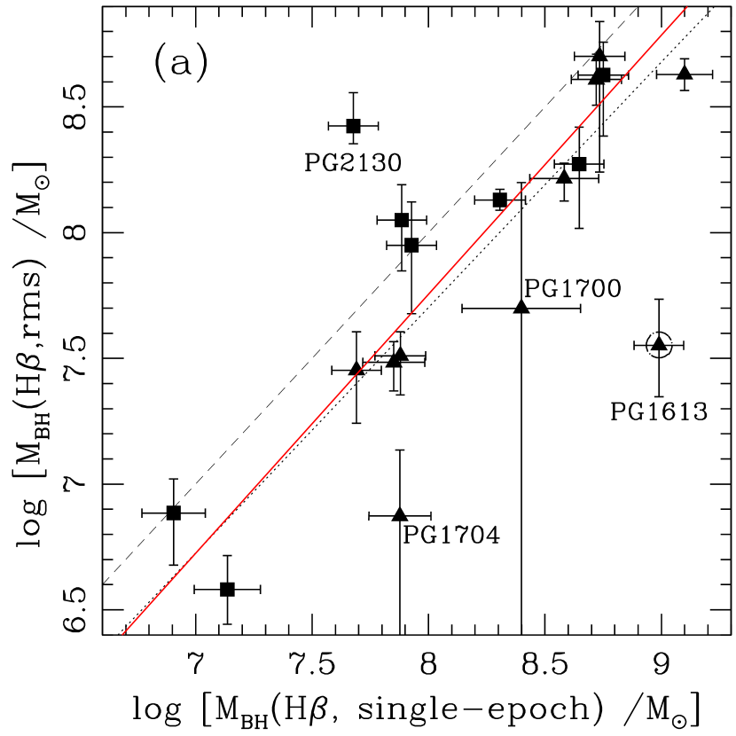
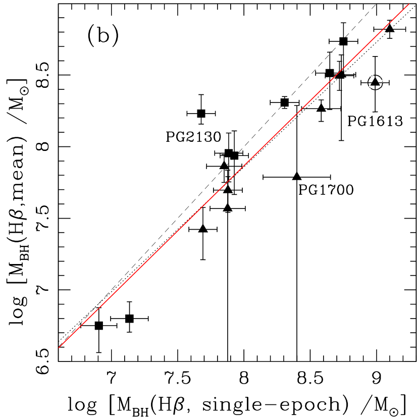
Figure 3: The reverberation masses derived from the rms (panel a) and mean (panel b) spectra plotted versus the single-epoch mass estimates based on optical spectral measurements. Triangles denote quasars, while squares denote Seyfert 1s. The dashed line indicates a unity relationship. The dotted line is a BCES bisector regression line to all the PG quasars with H $\beta$ measurements (shown), while the solid line is the BCES bisector when PG1613 is excluded (see text). As expected, $M_{\rm BH}(\rm H\beta,S$-E) show less scatter with $M_{\rm BH}(\rm H\beta,mean)$. Both relationships are consistent with a one-to-one relationship to within the errors.

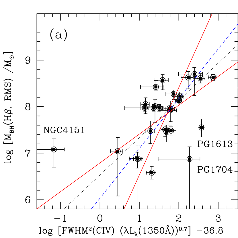
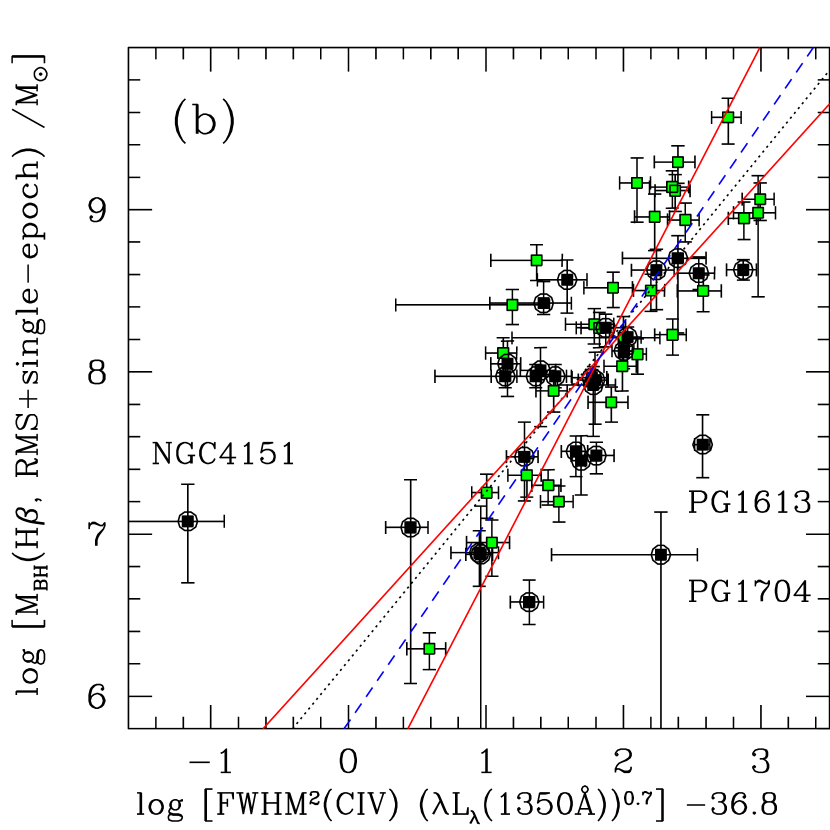
Figure 4: Established and estimated central masses based on optical data plotted versus the UV measurements. This distribution is the basis of the calibration of the UV measurements. The “optical masses” (ordinate) in panel (a) consist of the reverberation masses, $M_{\rm BH}(\rm H\beta,rms)$, (filled, circled squares) derived from the rms spectrum and based on H $\beta$ only. In panel (b) these masses are supplemented with the single-epoch mass estimates, $M_{\rm BH}(\rm H\beta,S$-E), (filled squares) for the 30 PG quasars with no reverberation mapping masses. Dotted lines: BCES bisector regression lines to all the objects in each diagram. Solid lines: BCES(Y$|$X) and (X$|$Y) regressions to all the objects except NGC 4151 (see text). Dashed lines: the BCES bisector for all objects excluding NGC 4151.

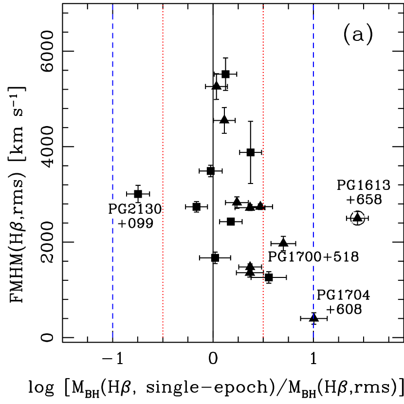
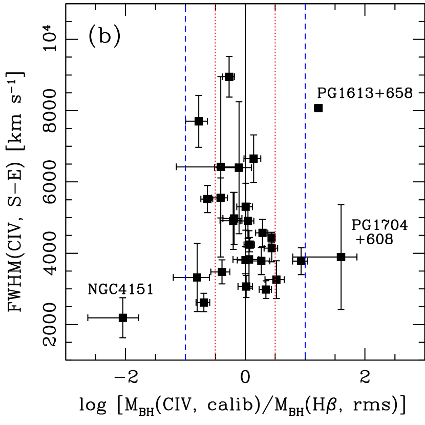
Figure 7: The mass deviations from Figure 8 plotted here versus the H $\beta$ and C iv line widths. The optical mass deviations are plotted against FWHM(H $\beta$, rms), the width of the rms profile (i.e., the variable part), in (a) and versus the single-epoch FWHM(C iv) in (b). Lines and symbols are as in Figure 8. Notice that the larger mass discrepancies tend to occur for the most narrow lined objects in both cases (or those with the strongest variability occurring in the narrow line core: PG1613$+$658 and PG1704$+$608).

References

- Adams, Graff, & Richstone (2001) Adams, F. C., Graff, D. S., & Richstone, D. O. 2001, ApJ, 551, L31
- Akritas & Bershady (1996) Akritas, M. G., & Bershady, M. A. 1996, ApJ, 470, 706
- (3) Blandford, R. D. 2001, in ASP Conf. Ser. 224, Probing the Physics of Active Galactic Nuclei by Multiwavelength Monitoring, ed. Peterson, B. M., Polidan, R. S., & Pogge, R. W. (San Francisco: ASP), 499
- Blandford & McKee (1982) Blandford, R. D., & McKee, C. F. 1982, ApJ, 255, 419
- (5) Boroson, T. A., & Green, R. F. 1992, ApJS, 80, 109 (BG92)
- (6) Brotherton, M. S. 1996, ApJS, 102, 1
- Burkert & Silk (2001) Burkert, A., & Silk, J. 2001, ApJ, 554, L151
- Clavel et al. (1991) Clavel, J., et al. 1991, ApJ, 366, 64
- (9) Collier, S., Peterson, B. M., & Horne, K. 2001, in ASP Conf. Ser. 224, Probing the Physics of Active Galactic Nuclei by Multiwavelength Monitoring, ed. Peterson, B. M., Polidan, R. S., & Pogge, R. W. (San Francisco: ASP), 457
- Dibai (1980) Dibai, E. A. 1980, Soviet Astronomy, 24, 389
- Fabian (1999) Fabian, A. C. 1999, MNRAS, 308, L39
- Feigelson & Babu (1992) Feigelson, E. D., & Babu, G. J. 1992, ApJ, 397, 55
- Ferland, Korista, & Peterson (1990) Ferland, G. J., Korista, K. T., & Peterson, B. M. 1990, ApJ, 363, L21
- (14) Ferrarese, L., & Merritt, D. 2000, 539, L9
- Ferrarese et al. (2001) Ferrarese, L., Pogge, R. W., Peterson, B. M., Merritt, D., Wandel, A., & Joseph, C. L. 2001, ApJ, 555, L79
- (16) Francis, P. J., Hewett, P. C., Foltz, C. B., Chaffee, F. H., Weymann, R. J., & Morris, S. L. 1991, ApJ, 373, 465
- Freedman et al. (2001) Freedman, W. L., et al. 2001, ApJ, 553, 47
- (18) Fromerth, M. J., Melia, F. 2000, ApJ, 533, 172
- (19) Gaskell, C. M. 1988, ApJ, 325, 114
- (20) Gebhardt, K., et al. 2000a, ApJ, 539, L13
- (21) Gebhardt, K., et al. 2000b, ApJ, 543, L5
- Gondhalekar (1990) Gondhalekar, P. M. 1990, MNRAS, 243, 443
- Green, Schmidt, & Liebert (1986) Green, R. F., Schmidt, M., & Liebert, J. 1986, ApJS, 61, 305
- Haehnelt & Kauffmann (2000) Haehnelt, M. G., & Kauffmann, G. 2000, MNRAS, 318, L35
- Ho (1999) Ho, L. C. 1999, in ASSL Vol. 234, Observational Evidence for the Black Holes in the Universe, ed. S. K. Chakrabarti (Dordrecht: Kluwer), 157
- Ho (2001) Ho, L. C. 2001, ApJ, submitted
- (27) Horne, K. 2001, in ASP Conf. Ser. 224, Probing the Physics of Active Galactic Nuclei by Multiwavelength Monitoring, ed. Peterson, B. M., Polidan, R. S., & Pogge, R. W. (San Francisco: ASP), 387
- Horne et al. (2002) Horne, K., Peterson, B. M., Collier, S. J., Netzer, H. 2002, PASP, submitted (astro-ph/0201182)
- Isobe, Feigelson, Akritas, & Babu (1990) Isobe, T., Feigelson, E. D., Akritas, M. G., & Babu, G. J. 1990, ApJ, 364, 104
- Jackson & Browne (1991) Jackson, N., & Browne, I. W. A. 1991, MNRAS, 250, 422
- (31) Kaspi, S. 2001, in ASP Conf. Ser. 224, Probing the Physics of Active Galactic Nuclei by Multiwavelength Monitoring, ed. Peterson, B. M., Polidan, R. S., & Pogge, R. W. (San Francisco: ASP), 347
- (32) Kaspi, S., Smith, P. S., Netzer, H., Maoz, D., Jannuzi, B. T., & Giveon, U. 2000, ApJ, 533, 631
- Kassebaum et al. (1997) Kassebaum, T. M., Peterson, B. M., Wanders, I., Pogge, R. W., Bertram, R., & Wagner, R. M. 1997, ApJ, 475, 106
- Kauffmann & Haehnelt (2000) Kauffmann, G., & Haehnelt, M. 2000, MNRAS, 311, 576
- (35) Kellerman, K. I., Sramek, R., Schmidt, M., Shaffer, D. B., & Green, R. 1989, AJ, 98, 1195
- (36) Kollatschny, W., & Welsh, W. F. 2001, in ASP Conf. Ser. 224, Probing the Physics of Active Galactic Nuclei by Multiwavelength Monitoring, ed. Peterson, B. M., Polidan, R. S., & Pogge, R. W. (San Francisco: ASP), 449
- (37) Koratkar, A. P., & Gaskell, C. M. 1991, ApJ, 370, L61
- Korista et al. (1995) Korista, K. T., et al. 1995, ApJS, 97, 285
- (39) Kormendy, J., & Gebhardt, K. 2001, in The 20th Texas Symposium on Relativistic Astrophysics, ed. H. Martel & J. C. Wheeler (AIP), 363
- Kormendy & Richstone (1995) Kormendy, J., & Richstone, D. 1995, ARA&A, 33, 581
- Krolik (2001) Krolik, J. H. 2001, ApJ, 551, 72
- Laor (1998) Laor, A. 1998, ApJ, 505, L83
- Laor (2000) Laor, A. 2000, ApJ, 543, L111
- Laor (2001) Laor, A. 2001, ApJ, 553, 677
- Laor et al. (1995) Laor, A., Bahcall, J. N., Jannuzi, B. T., Schneider, D. P., & Green, R. F. 1995, ApJS, 99, 1
- Laor et al. (1994) Laor, A., Bahcall, J. N., Jannuzi, B. T., Schneider, D. P., Green, R. F., & Hartig, G. F. 1994, ApJ, 420, 110
- Magorrian et al. (1998) Magorrian, J., et al. 1998, AJ, 115, 2285
- Marziani et al. (1996) Marziani, P., Sulentic, J. W., Dultzin-Hacyan, D., Calvani, M., & Moles, M. 1996, ApJS, 104, 37
- (49) McLure, R. J., & Dunlop, J. S. 2001, MNRAS, 327, 199
- (50) Merritt, D., & Ferrarese, L. 2001a, ApJ, 547, 140
- (51) Merritt, D., & Ferrarese, L. 2001b, in ASP Conf. Ser. 249 The Central kpc of Starbursts and AGN, ed. J. H. Knapen, J. E. Beckman, I. Shlosman, T. J. Mahoney (San Francisco: ASP), 335
- Nelson & Whittle (1995) Nelson, C. H., & Whittle, M. 1995, ApJS, 99, 67
- (53) Netzer, H. 2001, in ASP Conf. Ser. 224, Probing the Physics of Active Galactic Nuclei by Multiwavelength Monitoring, ed. Peterson, B. M., Polidan, R. S., & Pogge, R. W. (San Francisco: ASP), 335
- Netzer & Peterson (1997) Netzer, H., & Peterson, B. M. 1997, in ASSL Vol. 218, Astronomical Time Series, ed. D. Maoz, A. Sternberg, & E. M. Leibowitz (Dordrecht: Kluwer), 85
- (55) Neugebauer, G., Green, R. F., Matthews, K., Schmidt, M., Soifer, B. T., & Bennett, J. 1987, ApJS, 63, 615
- O’Brien, Zheng, & Wilson (1989) O’Brien, P. T., Zheng, W., & Wilson, R. 1989, MNRAS, 240, 741
- O’Brien et al. (1998) O’Brien, P. T., et al. 1998, ApJ, 509, 163
- Padovani, Burg, & Edelson (1990) Padovani, P., Burg, R., & Edelson, R. A. 1990, ApJ, 353, 438
- Padovani & Rafanelli (1988) Padovani, P., & Rafanelli, P. 1988, A&A, 205, 53
- Perez, Penston, & Moles (1989) Pérez, E., Penston, M. V., & Moles, M. 1989, MNRAS, 239, 75
- (61) Peterson, B. M. 2001a, in Advanced Lectures on The Starburst AGN connection, ed. I. Aretxaga, D. Kunth, & R. Mújica (Singapore: World Scientific), 3
- (62) Peterson, B. M. 2001b, in ASP Conf. Ser. 224, Probing the Physics of Active Galactic Nuclei by Multiwavelength Monitoring, ed. Peterson, B. M., Polidan, R. S., & Pogge, R. W. (San Francisco: ASP), 1
- (63) Peterson, B. M., & Wandel, A. 1999, ApJ, 521, L95
- (64) Peterson, B. M., & Wandel, A. 2000, ApJ, 540, L13
- Peterson et al. (1998a) Peterson, B. M., Wanders, I., Bertram, R., Hunley, J. F., Pogge, R. W., & Wagner, R. M. 1998a, ApJ, 501, 82
- Peterson et al. (1998b) Peterson, B. M., Wanders, I., Horne, K., Collier, S., Alexander, T., Kaspi, S., & Maoz, D. 1998b, PASP, 110, 660
- (67) Peterson, B. M., et al. 1999, ApJ, 510, 659
- Peterson et al. (2000) Peterson, B. M., et al. 2000, ApJ, 542, 161
- (69) Polidan, R. S., & Peterson, B. M. 2001, in ASP Conf. Ser. 224, Probing the Physics of Active Galactic Nuclei by Multiwavelength Monitoring, ed. Peterson, B. M., Polidan, R. S., & Pogge, R. W. (San Francisco: ASP), 479
- Richstone et al. (1998) Richstone, D., et al. 1998, Nature, 395, A14
- (71) Schmidt, M., & Green, R. F. 1983, ApJ, 269, 352
- Shields, Ferland, & Peterson (1995) Shields, J. C., Ferland, G. J., & Peterson, B. M. 1995, ApJ, 441, 507
- Silk & Rees (1998) Silk, J., & Rees, M. J. 1998, A&A, 331, L1
- Stirpe (1990) Stirpe, G. M. 1990, A&AS, 85, 1049
- Veron-Cetty & Veron (1993) Véron-Cetty, M. -P., & Véron, P. 1993, ESO Scientific Report (6th ed.; Garching: European Southern Observatory).
- Vestergaard (2000) Vestergaard, M. 2000, PASP, 112, 1504
- Vestergaard & Wilkes (2001) Vestergaard, M., & Wilkes, B. J. 2001, ApJS, 134, 1
- Wamsteker et al. (1990) Wamsteker, W., et al. 1990, ApJ, 354, 446
- (79) Wandel, A., 1999, ApJ, 519, L39
- (80) Wandel, A., 2001, in ASP Conf. Ser. 224, Probing the Physics of Active Galactic Nuclei by Multiwavelength Monitoring, ed. Peterson, B. M., Polidan, R. S., & Pogge, R. W. (San Francisco: ASP), 365
- (81) Wandel, A., & Mushotzky, R. F. 1986, ApJ, 306, L61
- (82) Wandel, A., Peterson, B. M., & Malkan, M. A. 1999, ApJ, 526, 579
- (83) Wandel, A., & Yahil, A. 1985, ApJ, 295, L1
- Wanders et al. (1997) Wanders, I., et al. 1997, ApJS, 113, 69
- (85) Wang, T.-G., Lu, Y.-J., Zhou, Y.-Y. 1998, ApJ, 493, 1
- (86) Welsh, W. F. 1999, PASP, 111, 1347
- (87) Wilkes, B. J., Kuraszkiewicz, J., Green, P. J., Mathur, S., McDowell, J. C. 1999, ApJ, 513, 76
- Wills, Netzer, & Wills (1985) Wills, B. J., Netzer, H., & Wills, D. 1985, ApJ, 288, 94
- Wills et al. (1995) Wills, B. J., et al. 1995, ApJ, 447, 139