On Optimal Detection of Point Sources in CMB Maps

Point-source contamination in high-precision Cosmic Microwave Background (CMB) maps severely affects the precision of cosmological parameter estimates. Among the methods that have been proposed for source detection, wavelet techniques based on “optimal” filters have been proposed (e.g., Sanz et al. 2001). In this paper we show that these filters are in fact only restrictive cases of a more general class of matched filters that optimize signal-to-noise ratio and that have, in general, better source detection capabilities, especially for lower amplitude sources. These conclusions are confirmed by some numerical experiments.

1 Introduction

The separation of different physical components is an important issue in the analysis of Cosmic Microwave Background (CMB) data. Among the foreground components, point-sources deserve especial attention given their extreme non-Gaussianity and highly variable spectral index. A brief summary of different methods can be found in Sanz et al. (2001) (henceforth SHM).

Methods used to detect point sources should act as high-pass filters to detect the high frequency structure introduced by the sources in the CMB data while masking other foreground contamination (like dust, synchrotron and free-free emission) characterized by lower frequencies. In principle, the good space/frequency characteristics of wavelets should make these functions an attractive choice for such tasks (e.g., Cayón et al. 2000; Vielva et al. 2001a, b, and references therein). Indeed, wavelets have been proved optimal for detection of point like singularities – at least for one-dimensional signals. Point sources in CMB maps, however, are not point singularities because the signal is smoothed by the beam of the antenna; sources are expected to have the shape of the antenna’s pattern. The question is then how to include this beam profile information in the wavelet analysis. SHM considered this question and, were lead to define optimal pseudo-filters for source detection in CMB maps. However, we show that nothing seems to be gained with these wavelet filters and that other simpler techniques lead to better source detection methods.

We first set up the basic framework. Although the detection of point-like sources in CMB maps is a two-dimensional problem, we present our arguments in $R^{n}$, as in SHM, because the same methods may be used in other applications.

The sources are assumed to be point-like signals convolved with the beam of the measuring instrument and are thus assumed to have a known profile $\tau(\boldsymbol{x})$. The signal $y(\boldsymbol{x})$, $\boldsymbol{x}\in R^{n}$, is modeled as

$$y(\boldsymbol{x})=\sum_{j}s_{j}(\boldsymbol{x})+z(\boldsymbol{x})$$ (1)

where

$$s_{j}(\boldsymbol{x})=A_{j}\,\tau(\boldsymbol{x}-\boldsymbol{x}_{j}),$$ (2)

$A_{j}$ and $\boldsymbol{x}_{j}$ are, respectively, unknown source amplitudes and locations, and $z(\boldsymbol{x})$ is a zero-mean background with power-spectrum $P(\boldsymbol{q})$

$${\rm E}\,[\,z(\boldsymbol{q})\,z^{*}(\boldsymbol{q}^{\prime})\,]=P(\boldsymbol{q})\leavevmode\nobreak\ \delta^{n}(\boldsymbol{q}-\boldsymbol{q}^{\prime}).$$ (3)

Henceforth ${\rm E}[\cdot]$ and “$\leavevmode\nobreak\ {}^{*}\leavevmode\nobreak\$” will denote the expectation and complex conjugate operators, respectively, $\delta^{n}(\boldsymbol{q}-\boldsymbol{q}^{\prime})$ the $n$-dimensional Dirac distribution, and $z(\boldsymbol{q})$ the Fourier transform of $z(\boldsymbol{x})$

$$z(\boldsymbol{q})=\int_{-\infty}^{+\infty}z(\boldsymbol{x})\leavevmode\nobreak\ {\rm e}^{-i\boldsymbol{q}\cdot\boldsymbol{x}}\leavevmode\nobreak\ \boldsymbol{d}\boldsymbol{x}.$$ (4)

To properly remove the point sources from the signal we need to estimate the locations $\{\boldsymbol{x}_{j}\}$ and amplitudes (fluxes) $\{A_{j}\}$ of the sources.

A classical method used to estimate source locations is based on identifying peaks in the cross-correlation function

$$c(\boldsymbol{x})=\int_{-\infty}^{+\infty}y(\boldsymbol{x}+\boldsymbol{b})\leavevmode\nobreak\ \tau(\boldsymbol{b})\leavevmode\nobreak\ \boldsymbol{d}\boldsymbol{b}.$$ (5)

The rationale is that $c(\boldsymbol{x_{o}})$ measures the similarity between the source profile with a section of $y(\boldsymbol{x})$ centered at $\boldsymbol{x_{o}}$; a peak in $c(\boldsymbol{x_{o}})$ is an indication of a source signal at $\boldsymbol{x_{o}}$. Eq. (5) is a filtering of the signal $y(\boldsymbol{x})$ with a filter $\tau(\boldsymbol{b})$ that amplifies the characteristic frequencies of the source. Once the sources have been located, their amplitudes can be estimated by means of classical fitting procedures like least squares.

The cross-correlation function (5) does not take into account the background characteristics. This is a great disadvantage in cases where the power spectrum $P(\boldsymbol{q})$ is known or a good estimate is available. In Sects. 2 and 3 we consider other methods that take into account this information and that may be considered extensions of the cross-correlation method.

The basic procedure we consider is as follows. The signal is first filtered to enhance the sources with respect to the background. This is done by cross-correlating the signal $y(\boldsymbol{x})$ with a filter $\Phi$ as in (5) (with $\Phi$ in place of $\tau$). The source locations are then determined by selecting the peaks in the filtered signal that are above a selected threshold. Finally, the source amplitudes are estimated with the values of the filtered signal at the estimated locations. The question we consider first is the selection of an optimal filter $\Phi$ for such procedure.

2 Designing an optimal filter

The optimality criteria we use are based on the following assumptions (for futher justification of these assumptions see SHM). The source profile and background spectrum are known. The profile is spherically symmetric, characterized by a scale $R_{s}$, and the background is assumed to be isotropic. In this case, we can write $s(\boldsymbol{x})\equiv s(x)$, where $x=\|\boldsymbol{x}\|$, and $P(\boldsymbol{q})\equiv P(q)$ for $q=\|\boldsymbol{q}\|$. In addition, source overlap is assumed negligible.

We consider the general family of spherically symmetric filters $\Phi(\boldsymbol{x};\boldsymbol{b})$ of the form

$$\Phi(\boldsymbol{x};\boldsymbol{b})=\phi(\,\|\boldsymbol{x}-\boldsymbol{b}\|\,)$$ (6)

with Fourier transform $\phi(q)$. The filtered field is

$$\begin{split}w(\boldsymbol{b};\phi)&=\int_{-\infty}^{+\infty}y(\boldsymbol{x})\leavevmode\nobreak\ \Phi(\boldsymbol{x};\boldsymbol{b})\leavevmode\nobreak\ \boldsymbol{d}\boldsymbol{x}\\ &=\int_{-\infty}^{+\infty}y(\boldsymbol{q})\leavevmode\nobreak\ \phi(q)\leavevmode\nobreak\ {\rm e}^{i\boldsymbol{q}\cdot\boldsymbol{b}}\leavevmode\nobreak\ \boldsymbol{d}\boldsymbol{q},\end{split}$$ (7)

where $y(\boldsymbol{q})$ and $\phi(q)$ are, respectively, the Fourier transforms of $y(\boldsymbol{x})$ and $\phi(\boldsymbol{x})$. The mean and variance of $w(\boldsymbol{b};\phi)$ are

$$\begin{split}\mu(\boldsymbol{b};\phi)&={\rm E}\,w(\boldsymbol{b};\phi)\\ &=\alpha\int_{0}^{+\infty}\!\!q^{n-1}\leavevmode\nobreak\ s(q)\,\phi(q)\,{\rm e}^{i\boldsymbol{q}\cdot\boldsymbol{b}}dq;\end{split}$$ (8)

$$\begin{split}\sigma^{2}(\phi)&={\rm E}\,w^{2}(\boldsymbol{b},\phi)-\mu(\boldsymbol{b};\phi)^{2}\\ &=\alpha\int_{0}^{+\infty}\!\!q^{n-1}\leavevmode\nobreak\ P(q)\,\phi(q)\leavevmode\nobreak\ dq,\end{split}$$ (9)

where $\alpha=2\,\pi^{n/2}\,\Gamma^{-1}(n/2)$.

The first constraint on the filter concerns the second stage of the procedure; the source locations are assumed known and the objective is to estimate the amplitudes. Given the assumed distance between sources, it is enough to consider a field $y(\boldsymbol{x})$ as in (1) with a single source at the origin, $s(\boldsymbol{x})=A\,\tau(\boldsymbol{x})$. To estimate its amplitude we ask that $w(\boldsymbol{0};\phi)$ be an unbiased estimator of $A$ – i.e., $\mu(\boldsymbol{0};\phi)=A$ – so that $\phi$ is required to satisfy the equation

$$\int_{0}^{+\infty}\!\!q^{n-1}\tau(q)\,\phi(q)\leavevmode\nobreak\ dq=\frac{1}{\alpha}.$$ (10)

To enhance the magnitude of the source relative to the background we determine the filter $\Phi$ that minimizes the variance $\sigma^{2}(\phi)$. This has the effect of maximizing, among unbiased estimators, the detection level

$$\mathcal{D}(\phi)=\frac{\mu(\boldsymbol{0};\phi)}{\sigma(\phi)},$$ (11)

which measures the capability of the filter to correctly detect a source at the prescribed location (see SHM).

Since $\Phi$ is chosen so that $w(\boldsymbol{0};\phi)$ is a minimum variance linear – in $y(\boldsymbol{x})$ – unbiased estimator of $A$, it follows that (Gauss-Markov theorem) $w(\boldsymbol{0};\phi)$ is the (generalized) least squares estimate of $A$ achieved by the filter

$$\phi(q)=\frac{1}{\alpha a}\leavevmode\nobreak\ \frac{\tau(q)}{P(q)},\qquad a\equiv\int_{0}^{+\infty}q^{n-1}\frac{\tau^{2}}{P}\leavevmode\nobreak\ dq,$$ (12)

with minimum variance

$$\sigma^{2}(\phi)=\frac{1}{\alpha a}.$$ (13)

Filter (12) is a particular case of a well known class of filters, known as matched filters in the engineering literature, that are designed to optimize signal-to-noise ratio (e.g., Kozma & Kelley 1965; Pratt 1991). The arguments in this section also show that the filter introduced by Tegmark & Oliveira-Costa (1998) is a particular case of the matched filter (12) with $P(q)$ representing the background power spectrum before the smoothing of the antenna.

For white noise, $P(q)={\rm const}=D$, filter (12) simplifies to

$$\phi(q)=\frac{1}{\alpha aD}\leavevmode\nobreak\ \tau(q)$$ (14)

which, up to a constant factor, is identical to the filter used in the classical cross-correlation function (5). This provides a justification for the use of the cross-correlation for source detection in white noise.

Having recognized $w(\boldsymbol{0};\phi)$ as a least squares estimator of $A$, we close this section with some remarks from least squares methodology that we consider relevant. First note that, regardless of the spectrum $P(q)$, the source profile $\tau(q)$ properly normalized, that is $\phi(q)=\tau(q)/K$ for $K=\alpha\,\int q^{n-1}\tau(q)\,\phi(q)\,{\rm e}^{i\boldsymbol{q}\cdot\boldsymbol{b}}\,dq$, also provides an unbiased estimator $w(\boldsymbol{0};\phi)$ of $A$. This is the (ordinary) least squares estimate that does not take into account the covariance of the background; it is unbiased but not minimum variance. However, it is well known that when the covariance is actually estimated from the data, the ordinary least squares estimate may be better than the generalized one (e.g., Draper & Smith 1998). In other words, uncertainities in the spectrum estimates may lead to worse amplitude estimates than those obtained with the simpler cross-correlation filter. Uncertainties in the spectrum will also affect the selection of a detection threshold.

Note also that the unbiasesness of $w(\boldsymbol{0};\phi)$ as an estimator of $A$ depends on knowing the correct source location, it is not necessarily unbiased once the source locations are estimated from the data. This is shown in Sect. 4.2.

3 Pseudo-filters

In the pseudo-filter approach of SHM the filters are of the form (6) with an additional scale dependence

$$\Psi(\boldsymbol{x};R,\boldsymbol{b})=\frac{1}{R^{N}}\,\psi\left(\frac{\|\boldsymbol{x}-\boldsymbol{b}\|}{R}\right),$$ (15)

for some spherically symmetric function $\psi$. From (15) we get a set of wavelets of different scales $R$ and shifts $\boldsymbol{b}$ provided the regularity conditions $\tau(q)/P(q)\rightarrow 0$, $(1/P)(d\tau/d\ln q)\rightarrow 0$ for $q\rightarrow 0$ are satisfied. The filtered field $w(\boldsymbol{b},R;\psi)$ at scale $R$ is defined as in (7) but with $\psi(Rq)$ in place of $\phi(q)$.

To determine an optimal filter $\psi$, SHM  minimize the variance of the filtered field subject to two constraints: First, $w(\boldsymbol{0},R_{0};\psi)$ is required to be, as in the previous section, an unbiased estimator of $A$ for some known $R_{0}\approx R_{s}$. For the second constraint $\psi$ is selected so that $\mu(\boldsymbol{0},R;\psi)$ has a local maximum at scale $R_{0}$. This constraint translates to

$$\int_{0}^{+\infty}q^{n-1}\tau(q)\,\psi(R_{0}q)\left(n+\frac{d\ln\tau}{d\ln q}\right)\leavevmode\nobreak\ dq=0.$$ (16)

Minimizing $\sigma^{2}(R_{0};\psi)$ with the two constraints yields the filter (SHM)

$$\psi(R_{0}q)=\frac{1}{\alpha\leavevmode\nobreak\ \Delta}\leavevmode\nobreak\ \frac{\tau(q)}{P(q)}\left[nb+c-(na+b)\,\frac{d\ln\tau(q)}{d\ln q}\right],$$ (17)

where $\Delta=ac-b^{2}$,

$$b \equiv\int_{0}^{+\infty}q^{n-1}\frac{\tau}{P}\leavevmode\nobreak\ \frac{d\tau}{d\ln q},$$ (18)

$$c \equiv\int_{0}^{+\infty}q^{n-1}\frac{1}{P}\left(\frac{d\tau}{d\ln q}\right)^{2}\leavevmode\nobreak\ dq,$$

and $a$ is as in (12). This filter provides a field of variance

$$\sigma^{2}(R_{0};\psi)=\frac{n^{2}a+2nb+c}{\alpha\Delta}.$$ (19)

The estimator of the amplitude $A$ obtained with this filter is again linear and unbiased and therefore, by the optimality of least squares, $\sigma^{2}(R_{0};\psi)\geq\sigma^{2}(\phi)$ regardless of the source profile and background spectrum. This means that the detection level of $\Phi$ is at least as high, or higher, than that achieved with $\Psi$.

3.1 Is $\Psi$ optimal for source detection?

We have seen that the second constraint (16) does not increase the detection level when the source locations are known. But this is not surprising since the constraint is defined to take advantage of the known source scale to help determine source locations. We will show that even when source location uncertainty is taken into account, (16) does not improve on the simpler filter $\Phi$ based on the single contraint (10). In other words, enough information about the scale of the source is already included in the derivation of the matched filter. Therefore, it seems that nothing is gained with wavelet methods.

In principle, as explained by SHM, constraint (16) can be used to test if a detection corresponds to a true source by checking for its maximum at scale $R_{0}$. But finding a spike at the correct scale is not enough to make sure it is not a spurious noise artifact, we have to follow it across scales to make sure that it scales appropriately. In any case, a similar test can also be designed for the matched filter: given that the source profile is assumed known, the matched filter leads to an amplitude versus scale dependence (see example in Sect. 4.1) that can be determined and used for such a test. This functional dependence provides more information than the existence of a local maxima and should, in the presence of noise, lead to better location estimates.

4 Examples

To compare the theoretical performances of the filters $\Phi$ and $\Psi$ we use the gain as defined by SHM

$$\begin{split}g(\psi,\phi)&={\mathcal{D}}(\phi)/\mathcal{D}(\psi,R_{0})\\ &=\sigma(R_{0};\psi)/\sigma(\phi),\end{split}$$ (20)

where $\mathcal{D}(\psi,R_{0})$ is as in (11) but defined for $\Psi(\boldsymbol{x};R_{0},\boldsymbol{0})$. We start with a specific example with Gaussian profiles and power-law spectra.

4.1 Gaussian sources and $P(q)=Dq^{-\gamma}$

Gaussian sources

$$\tau(q)=\theta^{n}\,{\rm e}^{-(q\theta)^{2}/\,2},$$ (21)

where $\theta$ is the “standard deviation” defining the scale, provide an important family of source profiles. Indeed, in many practical applications the instrument’s profile, and thus the point sources, are effectively characterized by Gaussian profiles. For the noise process we take the power-law spectrum $P(q)=Dq^{-\gamma}$. This family of spectra can be used to locally approximate spectra of other homogeneous processes and has as special cases white ($\gamma=0$) and $1/f$ ($\gamma=1$) noise processes.

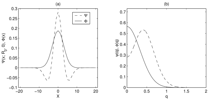
Figure 1: Filters $\Psi(x;R_{0},0)$ and $\Phi(x)$ for $n=1$ and white noise. Panel (a) shows the filters in spatial domain and panel (b) shows their power- spectra.

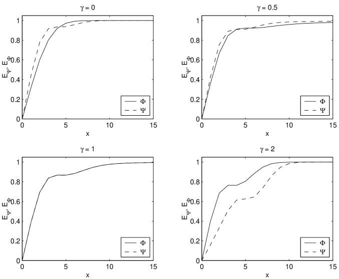
Figure 2: Cumulative energies $E_{\psi}$ and $E_{\phi}$ of $\Psi(x;R_{0},0)$ and $\Phi(x)$, respectively, for $n=1$ and different values of $\gamma$ (see text).

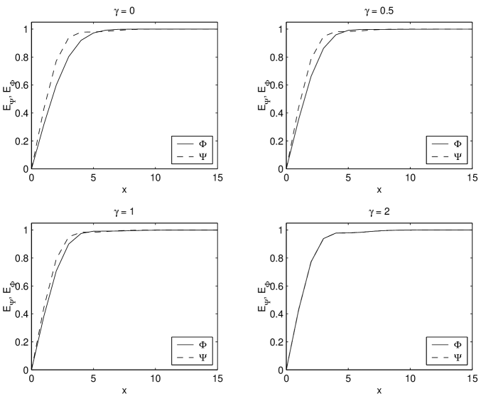
Figure 3: Same as Fig. 2 but with $n=2$.

	$S/N=1$				$S/N=2$				$S/N=3$
${\rm Filter}$	$N_{c}$	$N_{i}$	$A$		$N_{c}$	$N_{i}$	$A$		$N_{c}$	$N_{i}$	$A$
$\Psi$	23	10	1.83		87	10	1.10		100	10	0.97
	(15)	(5)	(1.94)		(80)	(5)	(1.14)		(100)	(5)	(0.98)
$\Phi$	31	5	1.55		97	5	1.02		100	5	0.98

Table 1: Results of the numerical simulations concerning the detection capabilities of the matched and the pseudo-filters (see text) in the one dimensional case and for a white noise background. $N_{c}$, $N_{i}$ are, respectively, the average number of correct and incorrect detections. Five hundred simulations were carried out using $100$ gaussian sources of amplitude $A=1$ and scale $\theta=3$, regularly distributed along an array of about $16000$ elements. The $3\sigma$ detection level has been determined by filtering, via $\Phi$ and $\Psi$, independent realizations of the background process. The amplitude estimates are based on the average amplitudes of all detected sources. The S/N is defined by $A/\sigma_{e}$ where $\sigma_{e}$ is the standard deviation of the noise process. The second row for $\Psi$ corresponds to results with a threshold ($>3\sigma$) chosen to achieve the same average number of incorrect detections as $\Phi$.

	$S/N=1$			$S/N=2$			$S/N=3$
${\rm Filter}$	$P_{c}$	$A$		$P_{c}$	$A$		$P_{c}$	$A$
$\Psi$	0.89	1.14		1.00	1.01		1.00	1.00
$\Phi$	0.99	1.03		1.00	1.00		1.00	1.00

Table 2: Results of two-dimensional simulations with a $128\times 128$ grid and white noise. $A$ is as in Table 1. $P_{c}$ is the estimated probability of correctly detecting a source keeping the rate of incorrect detection at the same level as in Table 1. Here $\Psi$ coincides with the Mexican hat wavelet.

	$S/N=1$			$S/N=2$			$S/N=3$
${\rm Filter}$	$P_{c}$	$A$		$P_{c}$	$A$		$P_{c}$	$A$
${\rm MH}$	0.38	1.79		0.93	1.11		1.00	1.03
$\Psi$	0.40	1.78		0.93	1.11		1.00	1.03
$\Phi$	0.47	1.60		0.97	1.07		1.00	1.02

Table 3: Results of two-dimensional simulations with a $128\times 128$ grid and $1/f$ noise. $A$ is as in Table 1. $P_{c}$ is the estimated probability of correctly detecting a source keeping the rate of incorrect detection at the same level as in Table 1. ${\rm MH}$ stands for Mexican hat wavelet.

For a Gaussian profile and a power-law spectrum, Eq. (12) leads to

$$\phi(q)=\frac{\Gamma(n/2)}{\Gamma(m)}\leavevmode\nobreak\ \frac{(q\theta)^{\gamma}}{\pi^{n/2}}\leavevmode\nobreak\ {\rm e}^{-(q\theta)^{2}/\,2},$$ (22)

where $m=(n+\gamma)/2$. ¿From (13) and (19) we obtain the following variance and gain

$$\sigma^{2}(\phi) =\frac{D}{\theta^{n-\gamma}\leavevmode\nobreak\ \pi^{n/2}}\leavevmode\nobreak\ \frac{\Gamma(n/2)}{\Gamma(m)},$$ (23)

$$\qquad g(\psi,\phi) =\left[\,1+\frac{(n-\gamma)^{2}}{4m}\,\right]^{1/2}.$$

We see that $g\geq 1$, which shows that $\phi$ has a higher detection level than $\psi$. For $n=\gamma$ —for example, one-dimensional process with $1/f$ noise— the two filters lead to the same detection levels. This is expected since $\phi(q)=\psi(Rq)$ for $n=\gamma$ (compare Eq. (22) with Eq. (24) in SHM). In other words, the second constraint is just redundant in this case. Note also that $\phi(q)$ is the Mexican hat wavelet for $n=2$ and $\gamma=2$. This results show that, contrary to what has been claimed before (e.g., Cayón et al. 2000), the optimality of the Mexican hat wavelet does depend on the background spectrum.

4.2 A numerical experiment

We have presented theoretical arguments showing that $\phi(q)$ has a better source detection capability than $\psi(Rq)$ when the source location is known. We now confirm that $\phi$ is still better when the uncertainity of source location estimates is taken into account. To compare with the results in SHM, it is enough to consider a simple example with one-dimensional Gaussian sources and white noise ($\gamma=0$) (we already know that $\phi=\psi$ for $n=1$ and $1/f$ noise). In this case (14) and (23) become, respectively,

$$\phi(q) =\frac{1}{\sqrt{\pi}}\leavevmode\nobreak\ {\rm e}^{-(q\theta)^{2}/\,2},$$ (24)

$$g(\psi,\phi) =\left(\frac{3}{2}\right)^{1/2}>1.$$

That is, the detection level of $\phi$ is about 20% larger than that of $\psi$. The amplitude dependence on $\theta$ of a Gaussian source of scale $R_{s}$ filtered with $\phi$ is

$$A(\theta)=\frac{\sqrt{2}\,R_{s}}{(\,R_{s}^{2}+\theta^{2}\,)^{1/2}}\,\,A.$$ (25)

A fit to this dependence can be used to determine if a detection corresponds to a source of the correct scale, just as large wavelet coefficients would be tracked across different wavelet scales.

Fig. 1 shows the filters $\Phi(\boldsymbol{x})$ and $\Psi(\boldsymbol{x};R_{0},\boldsymbol{0})$ and their corresponding Fourier transforms. It shows that the two filters are quite different. For example, to provide filtered sources with the scale $R_{0}$, $\psi$ has to pass higher frequencies than $\phi$. This can be a problem for signals contaminated by high frequency noise.

Table 1 shows the average number of correct and incorrect detections obtained with $\Psi$ and $\Phi$ and a fixed $3\sigma$ threshold for signal-to-noise (S/N) ratios equal to 1, 2 and 3. The two filters give equivalent results for higher S/N sources. We see that $\phi$ leads to a higher number of correct detections and a lower number of incorrect ones. But a proper comparison should take into account that the filters require different thresholds. The second row for $\Psi$ shows the corresponding results when the threshold is chosen to lead to the same average number of rejections as $\Phi$. For low S/N sources $\Phi$ leads again to a higher number of correct detections while for larger S/N they give similar results.

To compare amplitude estimates that include location uncertainty, we take the average of the amplitudes (since all the generated sources have the same amplitude) of all detections. The results are shown in Table 1. The errors in the amplitudes are of the order of 0.5% or less. We see that amplitude estimates are biased when the source locations are estimated, and that the bias is larger for $\Psi$. For low S/N the amplitude is overestimated because high peaks are easier to detect and noise peaks are incorrectly classified as sources. For high S/N sources we also have centering problems but this time the smaller amplitude in the noise peaks leads to underestimated source amplitudes. We can draw similar conclusions from the results of two-dimensional simulations shown in Tables 2 and 3;

To conclude, note that the spatial support of the filters is an important factor when the assumption of nonoverlapping filters is invalid. The support must be small compared to the distance between the sources. Figs. 2-3 show (for $n=1,2$) the cumulative energies

$${\rm E}_{\psi}(x)=\frac{\int_{0}^{x}\Psi^{2}(b;R_{0},0)db}{\int_{0}^{\infty}\Psi^{2}(b;R_{0},0)db}$$ (26)

and

$${\rm E}_{\Phi}(x)=\frac{\int_{0}^{x}\Phi^{2}(b)db}{\int_{0}^{\infty}\Phi^{2}(b)db},$$ (27)

as a function of $\gamma$ for a background spectrum $P(q)=Dq^{-\gamma}$. These functions measure the “energy concentration” of the filters and provide information about their “spatial” support. The figures show that also in this respect $\Phi(x)$ has similar, if not better, characteristics than $\Psi(x;R_{0},0)$. In particular, the filter $\Phi$ has a tighter support for faster decaying noise spectra.

4.2.1 Selecting the detection level

We briefly justify our selection of $3\sigma$ level. This threshold should be chosen large enough to reduce the number of false detections but small enough not to miss too many sources. To properly choose a threshold we have to understand the statistics of local maxima above a chosen level. For a general homogeneous (Gaussian) random field this is a difficult question (some asymptotic results can be found in Adler 1981) but simulations can be carried out when the background power spectrum is known. Our simulations showed that the traditional $5\sigma$ level is too conservative for the signal lengths used in the examples. If $P_{M}$ is the proportion of local maxima above $3\sigma$ for a field without sources. We found that the probability that $P_{M}$ is higher than 0.001 is about $9\%$ for the signal filtered with $\Psi$ and less than $10^{-5}$ for the signal filtered with $\Phi$.

5 Summary and Conclusions

We have revisited the problem of estimating point sources of known profile in an isotropic background. The methods we considered are based on two basic interrelated procedures: source detection by thresholding of local maxima, and amplitude estimation by linear filtering. We have compared the effects of different constraints on the selection of an optimal filter.

The first constraint is typical in matched filter methodology where S/N is maximized. The optimal filter provides unbiased least squares estimates of source amplitudes at known source locations. By the optimality of least squares, these amplitude estimates can not be improved with any other unbiased linear filter. However, uncertainities in source locations introduce a bias in amplitude estimates. Amplitudes are overestimated at low S/N and underestimated at high S/N. A second constraint introduced by SHM is designed to improve estimates of source locations by maximizing amplitudes at the correct scale. We found that this constraint does not lead to better estimates as compared to those obtained with a simpler matched filter, especially for lower S/N sources. For high S/N sources, as it was observed by Cayón et al. (2000), the results of the two methods are the same. These results contradict previous optimality studies of wavelet-based filters for detection of point-sources of known profile in an isotropic CMB background of known spectrum.

References

- Adler (1981) Adler, R. J. 1981, The Geometry of Random Fields (Wiley, New York)
- Cayón et al. (2000) Cayón, L. et al. 2000, MNRAS, 315, 757
- Draper & Smith (1998) Draper, N. R. & Smith, H. 1998, Applied Regression Analysis (Wiley, New York)
- Kozma & Kelley (1965) Kozma, A. & Kelly, D. L. 1965, Appl. Opt., 4, 387
- Pratt (1991) Pratt, W. K. 1991, Digital Image Processing (Wiley, New York)
- Sanz et al. (2001) Sanz, J. L., Herranz, D., & Martinez-Gonzalez, E. 2001, ApJ, 552, 484 (SHM)
- Tegmark & Oliveira-Costa (1998) Tegmark, M. & Oliveira-Costa, A. 1998, ApJ, 500L, 83
- Vielva et al. (2001a) Vielva, P. et al. 2001, MNRAS, 326, 181
- Vielva et al. (2001b) Vielva, P. et al. 2001, MNRAS, 328, 1