A possible contribution to CMB anisotropies at high $\ell$ from primordial voids

Abstract

We present preliminary results of an analysis into the effects of primordial voids on the cosmic microwave background (CMB). We show that an inflationary bubble model of void formation predicts excess power in the CMB angular power spectrum that peaks between $2000<\ell<3000$. Therefore, voids that exist on or close to the last scattering surface at the epoch of decoupling can contribute significantly to the apparent rise in power on these scales recently detected by the Cosmic Background Imager (CBI).

1 Introduction

One of the primary goals of modern cosmology is to gain an understanding of the formation and evolution of structure in the universe. Analyses of redshift surveys such as the 2-degree field galaxy redshift survey (2dFGRS, Peacock et al. 2001) suggest that there are large volumes of relatively empty space, or $voids$, in the distribution of galaxies. It seems that the universe is made up of a network of voids with most galaxies tending to be found in two dimensional sheets or filaments that surround these under-dense regions.

In the hierarchical model of structure formation, gravitational clustering is responsible for emptying voids of mass and galaxies (Peebles 1989). Simulations of the standard cold dark matter (CDM) model predict significant clumps of matter within voids that are capable of developing into observable bound objects (Dekel & Silk 1986; Hoffman et al. 1992). Peebles gives an in–depth discussion of the contradictions of this prediction with observation (Peebles 2001). He argues that the inability of the CDM models to produce the observed voids constitutes a true crisis for these models. Additionally, recently announced deep field observations from the Cosmic Background Imager (CBI) (Mason et al. 2002) show excess power on small angular scales, $\ell>2000$, in the cosmic microwave background (CMB).

It may be possible to explain the observations by postulating the presence of a void network originating from primordial bubbles of true vacuum that nucleated during inflation (La 1991; Liddle & Wands 1991; Turner et al. 1992; Occhionero & Amendola 1994; Amendola et al. 1996). In this scenario, the first bubbles to nucleate are stretched by the remaining inflation to cosmological scales. The largest voids may have had insufficient time to thermalize before decoupling and may persist to the present day. If voids exist at recombination they will leave an imprint on the cosmic microwave background. On the other hand, if they formed much later, their effect on the CMB will be negligible and will not be observed with the current generation of experiments.

The effects from primordial voids on the CMB have been investigated by a number of authors (Thompson & Vishniac 1987; Sato 1985; Martínez-González et al. 1990; Martínez-González & Sanz 1990; Liddle & Wands 1992; Panek 1992; Arnau et al. 1993; Mészáros 1994; Fullana et al. 1996; Mészáros & Molnár 1996; Shi et al. 1996; Baccigalupi et al. 1997; Amendola et al. 1998; Baccigalupi et al. 1998). The most complete investigation was carried out by Sakai et al. (1999) who modeled the effect for a distribution of equally sized voids.

In this Paper, we use a simple inflationary bubble model to show that if the voids that we see in galaxy surveys today existed at the epoch of decoupling, they would contribute significant additional power to the CMB angular power spectrum between $2000<\ell<3000$. Unlike previous analyses, we develop a general method that allows the creation of maps and enables us to consider an arbitrary distribution of void sizes. We model a power law distribution of void sizes as predicted by inflation (La 1991) and also take into account the finite thickness of the last scattering surface which suppresses part of the contribution from small voids.

2 Void networks in theory and observation

2.1 Predictions of the inflationary bubble model

In the extended inflationary model (La & Steinhardt 1989; see Kolb 1991 for a review), true vacuum bubbles nucleate during inflation in first order phase-transitions. This model predicts a distribution of bubble sizes greater than a given radius $r$ of the form,

$$N_{B}(>r)\propto r^{-\alpha}.$$ (1)

Typically, extended inflation is implemented within the framework of a Jordan-Brans-Dicke theory (Brans & Dicke 1961). In this case, the exponent $\alpha$ is directly related to the gravitational coupling $\omega$ of the scalar field that drives inflation,

$$\alpha=3+\frac{4}{\omega+1/2}.$$ (2)

Values of $\omega>3500$ are required by solar system experiments (Will 2001), although models have been proposed that either suppress or hide the present value of $\omega$ (La et al. 1989, Holman et al. 1990). The main driving force behind these models is that a low $\alpha$ can lead to large effects on the CMB if arbitrarily large voids are allowed (see Liddle & Wands 1991 for a review). The normalization of the bubble size distribution also depends on $\omega$ as well as on the energy scale of inflation.

Once formed, the bubbles will expand and form a shock wave on their boundary with the surrounding matter. After inflation ends, matter will start to flow relativistically back into the freshly created underdensities. However, cold dark matter only travels minimally into the void, since it becomes non-relativistic early on (Liddle & Wands 1992). Gravitational collapse of CDM will begin as normal at equality, further emptying any persisting voids. We expect baryonic matter to be pushed much further into the void as it is tightly coupled to relativistic photons until the epoch of decoupling when it will begin to gravitationally collapse back onto the CDM.

2.2 Void detections in redshift surveys

A number of different void finder algorithms have been developed to detect voids in redshift surveys (Kauffman & Fairall 1991; Kauffman & Melott 1992; Ryden 1995; Ryden & Melott 1996; El-Ad & Piran 1997; Aikio & Mähönen 1998). So far, such algorithms have been used to search for voids in the first slice of the Center for Astrophysics (CfA) redshift survey (Slezak et al. 1993), the Southern Sky Redshift Survey (SSRS) (Pellegrini et al. 1989, El-Ad et al. 1996), the Infra-Red Astronomical Satellite (IRAS) 1.2 Jy survey (El-Ad et al. 1997), the Las Campanas Redshift Survey (LCRS) (Müller et al. 2000), the Updated Zwicky Catalogue (UZC) (Hoyle & Vogeley 2002) and the Point Source Catalogue redshift (PSCz) survey (Plionis & Basilakos 2001, Hoyle & Vogeley 2002). These investigations indicate that 30-50% of the fractional volume of the universe is in the form of voids of underdensity $\delta\rho/\rho<-0.9$, in line with the inflationary model predictions. These voids range in radius from $r_{\rm min}$ = 10 $h^{-1}$ Mpc to $r_{\rm max}$ = 20-30 $h^{-1}$ Mpc.

3 The phenomenological void network model

We model the voids seen today as spherical underdensities of $\delta\rho/\rho=-1$. Each void is bounded by a thin wall containing the matter that is swept up during the void expansion. This forms a compensated void. We take the background universe to be an Einstein–de Sitter (EdS) cosmology, which is a good approximation since the majority of the effect on the CMB comes from voids on or close to the last scattering surface (LSS) and the universe tends towards an EdS cosmology at early times. Maeda & Sato (1983) and Bertschinger (1985) use conservation of momentum and energy respectively to show that these compensated voids will increase in radius $r_{v}$ between the onset of the gravitational collapse of matter at equality and the present day such that,

$$r_{v}(\eta)\propto\eta^{\beta}\,,$$ (3)

with $\beta\approx 0.39$ and where $\eta$ is conformal time.

In this Paper, we consider a phenomenological primordial void model that is based on the predictions of extended inflation with parameters chosen to be in agreement with current redshift survey observations; a full analysis of a larger family of models will be presented in a subsequent paper. Motivated by the inflationary scenario, we assume a power-law distribution of void sizes in the universe today, as given in equation (1). We further assume that the mechanism creating the voids imposes an upper cut-off on the size distribution. A possible mechanism for this cut-off could be that the tunneling probability of inflationary bubbles is modulated through the coupling to another field. We can therefore go to the limit of large $\omega$, leading to a spectrum of void sizes with $\alpha=3$. Apart from avoiding problems with well–established local measurements of gravity, this assumption allows us to match the observed upper limit on void sizes from the galaxy redshift surveys.

The minimal present void size is chosen to agree with redshift surveys, $r_{\rm min}=10\,h^{-1}$ Mpc. For the maximal radius, we choose the average value that is found, $r_{\rm max}=25\,h^{-1}$ Mpc. This scale can be strongly constrained by CMB data – if the maximal size were much larger, the voids would add too much additional power (given the observed value of $F_{v}$) at the wrong scales ($\ell<2000$). On the other hand, smaller voids would not be able to produce any significant contribution to the CMB power spectrum. The exponent of the size distribution $\alpha$ is weakly constrained by both theory and observations. Varying $\alpha$ changes the position of the peak and the overall power. This can partially adjust the influence of the other parameters (see figure 3).

We normalize the distribution by choosing the total number of voids so as to fill the required fraction of the universe today, $F_{v}$. Redshift surveys point to $F_{v}\approx 0.4$, ie. 40% of the volume of the universe is in underdense regions. The positions of the voids are then assigned randomly, making sure that they do not overlap. In order to speed up this process, we consider only a $10^{\circ}$ cone. This limits our analysis to $\ell>100$, which is satisfactory for our purpose since the main contribution from voids is on much smaller scales.

4 Stepping through the void network

4.1 Voids between us and the LSS

We ray trace photon paths from us to the LSS for the 10^∘ cone in steps of 1’. Each void in the present day distribution that is intersected by the photon path is evolved back in time according to (3) to determine whether the photon encounters the void. If a photon intersects a void between us and the LSS, we compute the Rees–Sciama (1968) effect due to the deviation in the redshift of the photon as it passes through the expanding void and the lensing effect due to the deviation in its path. Thompson & Vishniac (1987) applied double local Lorentz transformations at each void boundary to obtain the redshift deviation (the RS effect) and the scattering angle of a photon (the lensing effect),

$$\Delta_{\rm RS}\equiv\left.\frac{\delta T}{T}\right|_{\rm RS}=(H_{2}R_{2})^{3}\cos\theta_{2}\left(3\beta-\frac{2}{3}\cos^{2}\theta_{2}\right)\,,$$ (4)

$$\delta\alpha\equiv-\theta_{1}+\theta^{\prime}_{1}+\theta^{\prime}_{2}-\theta_{2}=(H_{2}R_{2})^{2}\sin(2\theta_{2})\,,$$ (5)

where $H$ is the Hubble parameter, $R\equiv ar_{v}$ is the proper length of the void radius, $\beta$ is given by (3) and the angles $\theta_{1}$, $\theta^{\prime}_{1}$, $\theta^{\prime}_{2}$ and $\theta_{2}$ are defined by reference to figure 1.

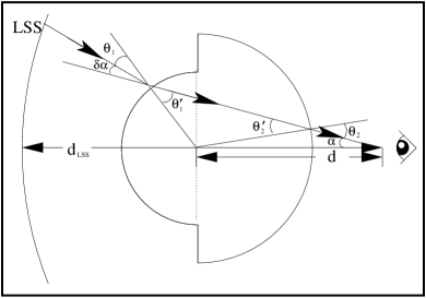
Figure 1: Cross section of a void (Thompson–Vishniac model). The trajectory of a photon is depicted from the LSS to an observer. The subscripts 1 and 2 denote quantities at the time the photon enters the void and at the time it leaves, respectively. $\alpha$ is defined as the angle formed between the line-of-sight direction and the direction of the void’s centre. $\delta\alpha$ is defined as the scattering angle of a photon. $d$ is defined as the comoving distance of the void’s centre. $d_{LSS}$ is defined as the comoving distance of the LSS.

This treatment agrees with the complementary approach of using the potential approximation for the under-density (Martínez-González et al. 1990). The potential approximation is defined in the EdS background making certain assumptions for which one of the Einstein equations reduces to the Poisson equation,

$$\frac{1}{a^{2}}\nabla^{2}\psi=4\pi G\bar{\rho}\,\delta\,,$$ (6)

where $\bar{\rho}$ is the background density and $\delta=\delta\rho/\bar{\rho}$ is the density fluctuation field. For a spherical void with a thin shell, $\rho(\eta,{\bf x})$ is explicitly written as,

$$\begin{array}[]{c}\rho(\eta,\,r)=\bar{\rho}(\eta)\theta(r-r_{v}(\eta))+\rho_{\rm in}(\eta,r)\theta(r_{v}(\eta)-r)\\ +\sigma(\eta)\delta_{\rm Dirac}(r-r_{v}(\eta))\,,\end{array}$$ (7)

where $\theta$ is the Heaviside function, $\delta_{\rm Dirac}$ is the Dirac delta function, $\rho_{\rm in}$ is the energy density inside the void, and $\sigma$ is the surface energy density of the shell. Using this model of a void and assuming $\rho_{\rm in}$ to be homogeneous, (6) is easily integrated to give,

$$\psi=\frac{1}{4}H^{2}a^{2}\left(r^{2}-r_{v}^{2}\right)\delta\,,\quad{\rm for}\quad r<r_{v}\,,$$ (8)

$$\psi=0\,,\quad{\rm for}\quad r>r_{v}\,.$$ (9)

The non-linear growth of the void causes the potential inside it to grow with respect to the EdS background. This gives rise to the RS effect given by,

$$\Delta_{\rm RS}=-2\int_{\rm LSS}^{0}d{\bf x}\cdot\nabla\psi\,.$$ (10)

The integration of (10) for a void between us at the LSS results in equation (4), that is the Thompson–Vishniac result.

4.2 Voids on the LSS

If a photon intersects a void on the LSS, we use the potential approximation to calculate the Sachs–Wolfe (1967) effect due to the photon originating from within the underdensity. For an empty void ($\delta=-1$) that satisfies the potential approximation (8), the SW effect is given by (Sakai et al. 1999),

$$\begin{array}[]{c}\Delta_{\rm SW}\equiv\left.\frac{\delta T}{T}\right|_{\rm SW}=\left.\frac{1}{12}H^{2}a^{2}\left(r_{v}^{2}-r^{2}\right)\right|_{\rm LSS}\\ =\frac{1}{12}H^{2}a^{2}\left(r_{v}^{2}\cos^{2}\theta_{2}-X^{2}\right)\,,\end{array}$$ (11)

where $X$ is defined as the distance between the centre of the void and the LSS. Equation (11) takes a maximal value at $r=0$ corresponding to the case where a photon originates at the void centre.

We take into account the finite thickness of the LSS, which suppresses the SW effect for small voids, by averaging the contribution from a number of photons originating from a LSS of mean redshift 1100 and standard deviation in redshift 80. We also calculate the partial RS effect (PRS) that arises due to the expansion of the void on the LSS as the photon leaves it. Using the potential approximation and integrating (10) we obtain,

$$\begin{array}[]{c}\Delta_{\rm PRS}\equiv\left.\frac{\delta T}{T}\right|_{\rm PRS}=2\left(3+\frac{\left(r_{2}^{2}-r_{\rm LSS}^{2}\right)+\eta_{2}\left(\eta_{2}-4\eta_{\rm LSS}\right)}{\eta^{2}_{\rm LSS}}\right.\\ \left.+2\log\left(\frac{\eta_{2}}{\eta_{\rm LSS}}\right)-2\frac{r_{2}\left(\eta_{2}-\eta_{\rm LSS}\right)^{2}\cos\theta_{2}}{\eta_{\rm LSS}^{2}\eta_{i}}\right)\,,\end{array}$$ (12)

where $r_{\rm LSS}$ and $r_{2}$ are the size of the void at $\eta_{\rm LSS}$ and at the time the photon leaves the void ($\eta_{2}$) respectively and the angle $\theta_{2}$ is defined by reference to figure 1.

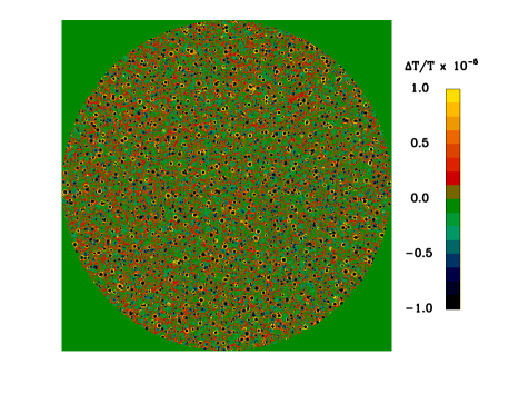
Figure 2: The map of the temperature fluctuations on the surface of last scattering from the fiducial void model considered. The parameters of this model are given by $\alpha=3$, $r_{\rm max}=25\,h^{-1}$ Mpc and $F_{v}=0.4$.

Once the photon has reached the last scattering surface, we know the variation of its temperature as well as its position on the LSS and can create a temperature map (figure 2). We then use a flat sky approximation to obtain the $C_{\ell}$ spectrum of the anisotropies (White et al. 1999; da Silva 2002) (see figure 3). This figure is the main result of this Paper and shows that a void model motivated by theory and observations can provide substantial power on scales beyond $\ell=2000$.

We point out that primordial void parameters are still poorly constrained by both observation and theory. The bottom panel of figure  3 shows a few further example models. For a power-law size distribution (as motivated by the inflationary scenario), large voids become rarer as $\alpha$ is increased. Therefore, since void analyses of redshift surveys only sample a fraction of the volume of the universe, there may exist voids of larger $r_{\rm max}$ than currently observed. Models with high $r_{\rm max}$ tend to predict too much power on scales $\ell\approx 1000$. However, if we take inflationary models with $\alpha>6$, as motivated by eg. Occhionero & Amendola (1994), then the peak moves to larger $\ell$ and the total power drops. The filling fraction mainly adjusts the overall power.

5 Conclusions

The cosmic microwave background is an excellent tool for probing the distribution of matter from last scattering until today. In the case of voids, the strongest signal stems from objects at very high redshifts, especially from those already present at decoupling. We discuss in this Paper the imprint of a power law distribution of primordial, spherical and compensated voids, which could for example be generated by a phase transition during inflation.

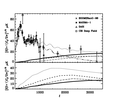
Figure 3: Top: The CMB anisotropies produced by the fiducial void model (solid line) compared to the primary CMB anisotropies (dashed-triple-dotted). Also plotted are the sum of primary and void contributions (dotted) as well as the fluctuations induced purely by voids on the last scattering surface (dashed) and by those between last scattering and today (dashed-dotted). We show the “standard” cosmological concordance model: of course a combined analysis of primary and void–induced fluctuations would select a different cosmology for the primary contribution. Bottom: Example models depicting a range of void contributions to the CMB fluctuations. The models plotted are $\alpha=3$, $r_{\rm max}=25\,h^{-1}$ Mpc and $F_{v}=0.4$ (solid line), $\alpha=3$, $r_{\rm max}=40\,h^{-1}$ Mpc and $F_{v}=0.4$ (dotted), $\alpha=3$, $r_{\rm max}=40\,h^{-1}$ Mpc and $F_{v}=0.2$ (dashed) and $\alpha=6$, $r_{\rm max}=40\,h^{-1}$ Mpc and $F_{v}=0.4$ (dashed-dotted).

We show that the signature of such a distribution of voids, that is compatible with redshift survey observations, contributes additional power on small angular scales. At the same time, this scenario solves the void–crisis of the CDM model. Experiments such as the CBI are able to directly probe small angular scales and constrain void parameters. We will present a constraints analysis of a wide range of void models in a future paper. In this in–depth analysis, we will also investigate the non-Gaussian signal of void models that are compatible with CMB observations as well as any effect of acoustic waves that primordial voids may propagate to the sound horizon (Baccigalupi & Perrotta 1998, Corasaniti et al. 2001).

Other sources are also expected to contribute at high $\ell$. Probably the strongest of these is the thermal Sunyaev-Zel’dovich (SZ) effect. Since the thermal SZ effect is strongly frequency–dependent, experiments which work at about 30 GHz (like CBI) will see a stronger signal than those working at higher frequencies (Aghanim et al. 2002). Hence a multi-frequency approach should be able to easily disentangle the contribution of voids from the SZ effect. Unfortunately, it seems to be difficult at present to predict the precise level of the SZ contribution, since different groups are reporting different results (see eg. Springel et al. 2000 for a compilation). Future multi-frequency, high-resolution and high signal-to-noise maps should be able to significantly constrain the contribution of primordial voids to the high $\ell$ CMB power spectrum. Additionally, deep galaxy redshift surveys and measurements of the distribution of matter in the Ly-$\alpha$ forest will able to directly explore the presence of voids in the baryonic matter distribution at low redshifts.

References

- [1] Aghanim N. et al., 2002, preprint archived under astro-ph/0203112.
- [2] Aikio J. and Mähönen P., 1998, Astrophys. J. 497, 534.
- [3] Amendola L. et al., 1996, Phys. Rev. D 54, 7199.
- [4] Amendola L., Baccigalupi C. and Occhionero F., 1998, Astrophys. J. 492, L5.
- [5] Arnau J.V. et al., 1993, Astrophys. J. 402, 359.
- [6] Baccigalupi C., Amendola L. and Occhionero F., 1997, Mon. Not. R. Astron. Soc. 288, 387.
- [7] Baccigalupi C., 1998, Astrophys. J. 496, 615.
- [8] Baccigalupi C., Perrotta F., 2000, Mon. Not. R. Astron. Soc., 314, 1
- [9] Bertschinger E., 1985, Astrophys. J. Supp. 58, 1.
- [10] Brans C. and Dicke C.H., 1961, Phys. Rev. 24, 925.
- [11] Corasaniti P.S., Amendola L. and Occhionero F., 2001, Mon. Not. R. Astron. Soc., 323, 677
- [12] Dekel A. and Silk J., 1986, Astrophys. J. 303, 39.
- [13] El-Ad H. et al., 1996, Astrophys. J. Lett. 462, L13.
- [14] El-Ad H., Piran T. and Dacosta L.N., 1997, Mon. Not. R. Astron. Soc. 287, 790.
- [15] El-Ad H. and Piran T., 1997, Astrophys. J. 491, 421.
- [16] Fullana M.J., Arnau J.V. and Saez D., 1996, Mon. Not. R. Astron. Soc. 280, 1181.
- [17] Hoffman Y., Silk J. and Wyse R.F.G., 1992, Astrophys. J. Lett. 388, L13.
- [18] Holman R., Kolb E.W. and Wang Y., 1990, Phys. Rev. Lett. 65, 17.
- [19] Hoyle F. and Vogeley M.S., 2002, Astrophys. J. 566, 641.
- [20] Kauffmann G. and Fairall A.P., 1991, Mon. Not. R. Astron. Soc. 248, 313.
- [21] Kauffmann G. and Melott A.L., 1992, Astrophys. J. 393, 415.
- [22] Kolb E.W., 1991, in The Birth and Early Evolution of the Universe, Proceedings of the 1990 Nobel Symposium.
- [23] La D. and Steinhardt P.J., 1989, Phys. Rev. Lett. 62, 376.
- [24] La D., Steinhardt P.J. and Bertschinger E., 1989, Phys. Lett. B 231 231.
- [25] La D., 1991, Phys. Lett. B 265, 232.
- [26] Liddle A.R. and Wands D., 1991, Mon. Not. R. Astron. Soc. 253, 637.
- [27] Liddle A.R. and Wands D., 1992, Phys. Lett. B 276, 18.
- [28] Maeda K. and Sato H., 1983, Progr. Theor. Phys. 70, 772.
- [29] Martínez-González E., Sanz J.L. and Silk J., 1990, Astrophys. J. Lett 355, 5.
- [30] Martínez-González E. and Sanz J.L., 1990, Mon. Not. R. Astron. Soc. 247, 473.
- [31] Mason B.S. et al., 2002, astro-ph/0205384
- [32] Mészáros A., 1994, Astrophys. J. 423, 19.
- [33] Mészáros A. and Molnár Z., 1996, Astrophys. J. 470, 49.
- [34] Müller V. et al., 2000, Mon. Not. R. Astron. Soc. 318, 280.
- [35] Occhionero F. and Amendola L., 1994, Phys. Rev. D 50, 4846.
- [36] Panek M., 1992, Astrophys. J. 388, 225.
- [37] Peacock J.A. et al., 2001, Nature 410, 169.
- [38] Peebles P.J.E., 1989, J. R. Astron. Soc. Canada 83, 363.
- [39] Peebles P.J.E., 2001, Astrophys. J. 557, 495.
- [40] Pellegrini P.S., da Costa L.N. and de Carvalho R.R., 1989, Astrophys. J. 339, 595.
- [41] Plionis M. and Basilakos S., 2002, Mon. Not. R. Astron. Soc. 330, 399.
- [42] Ryden B.S., 1995, Astrophys. J. 452, 25.
- [43] Ryden B.S. and Melott A.L., 1996, Astrophys. J. 470, 160.
- [44] Rees M.J. and Sciama D., 1968, Nature 217, 511 (1968).
- [45] Sachs R.K. and A.M. Wolfe A.M., 1967, Astrophys. J. 147, 73.
- [46] Sakai N., Sugiyama N. and Yokoyama J., 1999, Astrophys. J. 510, 1.
- [47] Sato H., 1985, Prog. Theor. Phys. 73, 649.
- [48] Shi X., Widrow L.M. and Dursi L.J., 1996, Mon. Not. R. Astron. Soc. 281, 565.
- [49] da Silva A., 2002, DPhil Thesis, University of Sussex (in preparation).
- [50] Slezak E., de Lapparent V. and Bijaoui A., 1993, Astrophys. J. 409, 517.
- [51] Springel V., White M. and Hernquist L., 2001, Astrophys. J. 549, 681; ibid. Astrophys. J. 562, 1086.
- [52] Thompson K.L. and Vishniac E.T., 1987, Astrophys. J. 313, 517.
- [53] Turner M.S., Weinberg E.J. and Widrow L.M., 1992, Phys. Rev. D 46, 2384.
- [54] White M., Carlstrom J.E., Dragovan M. & Holzapfel W.L., 1999, Astrophys. J. 514, 12
- [55] Will C.M., 2001, Living Rev. Rel. 4, 4.