Microarcsecond Radio Imaging using Earth Orbit Synthesis

Abstract

The observed interstellar scintillation pattern of an intra-day variable radio source is influenced by its source structure. If the velocity of the interstellar medium responsible for the scattering is comparable to the earth’s, the vector sum of these allows an observer to probe the scintillation pattern of a source in two dimensions and, in turn, to probe two-dimensional source structure on scales comparable to the angular scale of the scintillation pattern, typically $\sim 10\,\mu$as for weak scattering. We review the theory on the extraction of an “image” from the scintillation properties of a source, and show how earth’s orbital motion changes a source’s observed scintillation properties during the course of a year. The imaging process, which we call Earth Orbit Synthesis, requires measurements of the statistical properties of the scintillations at epochs spread throughout the course of a year.

1 Introduction

Flux density variability on intra-day timescales has recently been detected in a few tens of extragalactic radio sources (Heeschen 1984; Witzel et al. 1986, Kedziora-Chudczer et al. 2001). There is now overwhelming evidence that the principal mechanism responsible for intra-day variability (IDV) at centimeter wavelength is interstellar scintillation (ISS), rather than intrinsic source variability (Kedziora-Chudczer et al.  1997; Dennett-Thorpe & de Bruyn 2001a,b; Jauncey et al. 2001; Rickett et al.  2001; Jauncey & Macquart 2001).

ISS is observed in compact ($\lesssim 100\,\mu$as) radio sources due to the scattering of radiation in the Galactic interstellar medium (ISM) as it propagates toward earth. Inhomogeneities in the ISM impart phase structure on the wavefront, which leads in turn to a pattern of flux density deviations on the observer’s plane. Flux density variability is observed in a scattered source if an observer moves relative to the source’s scintillation pattern, ie. due to relative motion between the ISM, the source and the earth. The presence of such radio IDV implies extremely small source sizes ($\sim 5-100\,\mu$as), and high brightness temperatures ($T_{B}\sim 10^{13}-10^{15}$ K, e.g. Kedziora-Chudczer et al. 1997). This is well above the inverse Compton limit, and it is not clear whether such emission is explainable in terms of Doppler boosted synchrotron emission (Begelman, Rees & Sikora 1994). The properties — including the radio structures — of IDV sources are therefore of considerable interest.

The scintillation pattern of an IDV source contains information on the structure of the source, which can be derived from the statistical properties of the scintillation pattern given the statistical properties of the scattering medium. This has already been demonstrated for sources undergoing interplanetary scintillation; the experiment by Cornwell, Anantharamaiah & Narayan (1989) is an elegant illustration of this technique.

Some IDV sources exhibit large annual modulations in their variability timescales (Dennett-Thorpe & de Bruyn 2001a; Rickett et al. 2001; Jauncey & Macquart 2001). This is explained in terms of the earth’s orbital motion; as the earth’s velocity changes during its orbit about the sun, so does an earth-based observer’s velocity relative to the ISM. Both the speed and direction change greatly if the speed of the scintillation pattern relative to the heliocentre, due to the intrinsic motion of the ISM, is comparable to the earth’s speed. This effect is expected to be prevalent for IDV sources because the ISM velocity is comparable to earth’s, but is not generally observed in the scintillations of pulsars because of their high intrinsic speeds. Their speeds, typically $\gtrsim 150$ km/s are much greater than that of the earth or the ISM, and usually dominate the scintillation speed.

The large variation in scintillation speed and direction over the course of a year makes it possible to observe two-dimensional structure in the scintillation pattern. Hence ISS can be used to “image” a source on $5-100\,\mu$as scales. In this paper we show how to use changes in the earth’s velocity around the sun to probe the scintillation pattern in two dimensions, and how to invert this information to obtain source structure. We refer to this technique as Earth Orbit Synthesis in light of its similarity to the conventional radio interferometric imaging technique of Earth Rotation Synthesis.

As for the radio imaging technique of Earth Rotation Synthesis, Earth Orbit Synthesis assumes that the source structure remains relatively stable over the course of the observations. This appears to be a good assumption for several IDV sources that have been well-studied over a number of years. B0917$+$624 appears to have been scintillating over the decade and a half that this source has been followed in detail (e.g. Jauncey & Macquart 2001), while J1819$+$3845 has shown a clear annual cycle that repeats closely over at least the last two years (Dennett-Thorpe & de Bruyn 2001a), and PKS 1519$-$273 has shown IDV each time it has been observed in sufficient detail over the past decade (Kedziora-Chudczer et al. 2001). However, it should be remembered that this technique is not applicable to those sources that exhibit episodic IDV such as PKS 0405$-$385 (Kedziora-Chudczer et al. 2000).

In §2 the apparent scintillation velocity of an extragalactic source is derived in terms of the velocities of the ISM and the earth. In §3 we relate the statistics of intensity and polarization fluctuations to source structure. A model for the scintillation velocity is combined with statistics of the intensity fluctuations to derive source structure in §4, and the technique is demonstrated with some specific examples. The conclusions are presented in §5.

2 Earth’s orbital motion

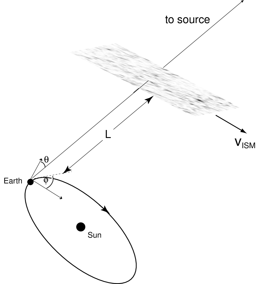
Figure 1: The scattering model. The earth-source line of sight moves relative to a scattering screen, fixed at a distance $L$ from earth.

The velocity of an earth-based observer across the scintillation pattern of a scattered source varies annually due to the earth’s orbit about the sun. Here we derive the observed scintillation velocity in terms of the position of a distant scintillating source and the velocity of the interstellar medium relative to the heliocentre (see Fig. 1).

We assume that the internal motions of the scattering material are negligible compared to the bulk motion of the material across the line of sight. We also assume that the scattering occurs predominantly in one layer of the ISM only, at a distance $L$ from earth, so that motion of the scattering material can be characterized by a single velocity. This assumption appears to be valid for a few IDV radio sources whose scattering screens appear to be nearby and localized (e.g. Dennett-Thorpe & de Bruyn 2000), and is a good approximation for other IDV sources.

The observed velocity of the line of sight to an extragalactic source through a scattering screen is given by

$${\bf v}_{\rm obs}={\bf v}_{\rm ISM}-{\bf v}_{\hbox{$\oplus$}},$$ (2-1)

where ${\bf v}_{\rm ISM}=({v_{\rm ISM}}_{x},{v_{\rm ISM}}_{y},{v_{\rm ISM}}_{z})$ and ${\bf v}_{\hbox{$\oplus$}}$ are, respectively, the velocities of the ISM and the earth relative to the heliocentre. For extragalactic sources, the proper motions of the source across the line of sight can be ignored. The co-ordinate system is aligned so that ${\bf e}_{z}$ points normal to the ecliptic plane and ${\bf e}_{x}$ points along ecliptic longitude $0^{\circ}$ in the ecliptic plane.

We ignore the $0.01^{\circ}$ inclination of the earth’s orbit to the ecliptic, and approximate the earth’s orbital motion as occurring in the ecliptic plane. The eccentricity of the earth’s orbit ($e=0.0167$) results in a negligible variation in orbital speed. We therefore approximate the earth’s orbital velocity relative to the heliocentre as:

$${\bf v}_{\hbox{$\oplus$}} = v_{\hbox{$\oplus$}}(\sin 2\pi t,-\cos 2\pi t,0),$$ (2-2)

where $v_{\hbox{$\oplus$}}=29.78\,$km/s is the mean orbital speed of the earth, $t$ is the time in years measured from the vernal equinox.

As shown in Figure 1, and choosing the earth to be at the origin of the co-ordinate system we write location of the scintillation screen in terms of ecliptic co-ordinates ${\bf a}=a\,(\cos\phi\cos\theta,\sin\phi\cos\theta,\sin\theta)$, where $\phi$ and $\theta$ are, respectively, the ecliptic longitude and latitude of the scintillating source. For typical screen distances $\gtrsim 20$pc, changes in $\hat{\bf a}={\bf a}/a$ caused by orbital changes in the earth’s position relative to the screen are negligible.

The observed motion of the scintillation pattern across the line of sight is

$${\bf v}_{\rm scint}=[V_{\parallel}+v_{\hbox{$\oplus$}}\cos(2\pi t-\phi)]{\bf e}_{\parallel}+[V_{\perp}+v_{\hbox{$\oplus$}}\sin\theta\sin(2\pi t-\phi)]{\bf e}_{\perp},$$ (2-3)

where ${\bf e}_{\parallel}=(-\sin\phi,\cos\phi,0)$ and ${\bf e}_{\perp}=(-\cos\phi\sin\theta,-\sin\phi\sin\theta,\cos\theta)$ are, respectively, the unit vectors parallel and perpendicular to the ecliptic along the line of sight to the scintillating source. The intrinsic speed of the ISM relative to the heliocentre and tangential to the line of sight is $V_{\parallel}$ along ${\bf e}_{\parallel}$ and $V_{\perp}$ along ${\bf e}_{\perp}$, where

$$V_{\parallel} = {v_{\rm ISM}}_{y}\cos\phi-{v_{\rm ISM}}_{x}\sin\phi,$$ (2-4)

$$V_{\perp} = {v_{\rm ISM}}_{z}\cos\theta-\sin\theta({v_{\rm ISM}}_{x}\cos\phi+{v_{\rm ISM}}_{y}\sin\phi).$$ (2-5)

Equation (2-3) implies that the velocity of the scintillation pattern relative to the earth changes in both magnitude and direction on an annual cycle.

3 Source structure

The scintillation pattern of a scattered source is related to both its intrinsic structure and the inhomogeneities in the ISM. Source structure can be derived if the statistical properties of the scintillation pattern due to a point-source are known. In §3.1 we express for the scintillation pattern due to a point source in terms of the scattering medium’s statistical properties. In §3.2 we show how the scintillation pattern is modified when the scintillating source has extended structure.

3.1 The scintillation pattern of a point source

The scintillation pattern of a point source depends upon the phase fluctuations on the scattering screen which are characterized by the phase structure function

$$D_{\phi}({\bf r})=\langle[\phi({\bf r}^{\prime}+{\bf r})-\phi({\bf r}^{\prime})]^{2}\rangle.$$ (3-1)

The angular brackets denote an ensemble average over all possible realisations of the scattering medium, and ${\bf r}$ is a two-dimensional vector on the scattering screen.

For most lines of sight through the ISM the phase structure function reflects an underlying power law spectrum of phase inhomogeneities between some inner and outer scales $l_{0}$ and $L_{0}$ respectively, and one has

$$D_{\phi}({\bf r})=\left(\frac{r}{r_{\rm diff}}\right)^{\beta-2},$$ (3-2)

where $\beta$ is close to $11/3$ (Armstrong, Rickett & Spangler 1995), the value expected for Kolmogorov turbulence. The strength of the phase fluctuations is measured by $r_{\rm diff}$, the length scale over which the root-mean-square phase difference on the phase screen is one radian.

The strength of the scattering is determined by the ratio $r_{\rm F}/r_{\rm diff}$; the quantity $r_{\rm F}=\sqrt{cL/(2\nu\pi)}$ is the Fresnel scale. The scattering is weak when phase irregularities on the scattering screen are small, when $r_{\rm diff}>r_{\rm F}$ and strong when they are large, when $r_{\rm diff}<r_{\rm F}$. The scattering strength varies as a function of frequency since both $r_{\rm diff}\propto\nu^{2/(\beta-2)}$ and $r_{\rm F}$ vary with frequency. It is convenient to define $\nu_{t}$ as the frequency at which the scattering changes from strong to weak. The scattering is weak at frequencies above $\nu_{t}$, while strong scattering occurs at frequencies below $\nu_{t}$.

The qualitative properties of the scintillation depend heavily on the scattering strength, and hence on $\nu_{t}$. In general, the value of $\nu_{t}$ toward a scintillating source is unknown, but can be determined from observations of its variability over a range of frequencies (e.g. Kedziora-Chudczer et al. 1997; Quirrenbach et al. 2000; Kedziora-Chudczer et al. 2001), or can be inferred from models of the ISM (Walker 1998). Along lines of sight out of the Galactic plane the transition frequency is in the range $\nu_{t}\sim 3-8$ GHz (Walker 1998).

A useful statistic of the intensity fluctuations of a point source due to scattering by the ISM is the intensity autocorrelation function

$${C_{II}}_{\rm pt}({\bf r})=\langle\delta I_{\rm pt}({\bf r}^{\prime}+{\bf r})\delta I_{\rm pt}({\bf r}^{\prime})\rangle,$$ (3-3)

where $\delta I_{\rm pt}({\bf r})=[I({\bf r})-\langle I\rangle]/\langle I\rangle$ is the fractional deviation in the intensity at the point ${\bf r}$ on the observer’s plane. This function describes the correlation between the intensity fluctuations between points ${\bf r}^{\prime}$ and ${\bf r}^{\prime}+{\bf r}$ on the observer’s plane. An alternative but equivalent representation of the intensity fluctuations is provided by the power spectrum, ${W_{II}}_{\rm pt}$, which is related to the intensity autocorrelation function by a Fourier transform

$${W_{II}}_{\rm pt}=\int d^{2}{\bf r}\exp[i{\bf q}\cdot{\bf r}]{C_{II}}_{\rm pt}({\bf r}).$$ (3-4)

We adopt the power spectrum representation in the discussion below.

The functional dependence of ${W_{II}}_{\rm pt}({\bf r})$ depends on the scattering strength. In the regime of weak scattering, one has (Salpeter 1967, Jokipii & Hollweg 1970, Narayan 1992)

$${W_{II}}_{\rm pt}({\bf q}) = C\,q^{-2}\left(\frac{1}{qr_{\rm diff}}\right)^{\beta-2}\sin^{2}\left(\frac{1}{2}r_{\rm F}^{2}q^{2}\right),$$ (3-5)

with $C=11.2$ for $\beta=11/3$. The power spectrum peaks at $q\sim 1/r_{\rm F}$, showing that the typical length scale of scintillations in the regime of weak scattering is $r\approx r_{\rm F}$. An object undergoing weak scintillations would exhibit flux density variations on a timescale $t_{\rm F}=r_{\rm F}/v_{\rm scint}$.

In the regime of strong scattering the power spectrum of intensity fluctuations for $\beta<4$ is (Gochelashvily & Shishov 1975)

$${W_{II}}_{\rm pt}(q)=\left\{\begin{array}[]{ll}2^{\beta-3}\frac{\pi(\beta-2)(4-\beta)\Gamma(\beta/2)}{\Gamma\left(\frac{6-\beta}{2}\right)}\,q^{-2}\left(\frac{r_{\rm F}}{r_{\rm diff}}\right)^{\beta-2}(qr_{\rm F})^{6-\beta}\exp[-(qr_{\rm ref})^{\beta-2}],&q\lesssim r_{\rm ref}^{-1}\\ \frac{2\pi}{\beta-2}\,\Gamma\left(\frac{1}{\beta-2}\right)r_{\rm diff}^{2},&r_{\rm ref}^{-1}\lesssim q\lesssim r_{\rm diff}^{-1}\\ \frac{2^{\beta}\pi(\beta-2)\Gamma(\beta/2)}{\Gamma\left(\frac{4-\beta}{2}\right)}\,q^{-2}(qr_{\rm diff})^{2-\beta},&r_{\rm diff}^{-1}\lesssim q\\ \end{array}\right.,$$ (3-9)

where $r_{\rm ref}=r_{\rm F}^{2}/r_{\rm diff}$ is known as the refractive scale. Intensity fluctuations can occur predominantly on two timescales in this regime, corresponding to the two peaks in ${W_{II}}_{\rm pt}(q)$. The outermost peak, corresponding to the effect of diffractive scintillation, occurs at $q\sim 1/r_{\rm diff}$ and is associated with fast-timescale, narrowband, large amplitude (up to 100% modulated) variability.

The other peak in ${W_{II}}_{\rm pt}(q)$ occurs at $q\sim 1/r_{\rm ref}$, and is associated with refractive scintillation. Refractive scintillations occur on a longer timescale than weak scintillations, are broadband and have a typically low ($\sim 10$%) modulation index. The timescale associated with refractive scintillation is $t_{\rm ref}=r_{\rm ref}/v_{\rm scint}$. This is a factor $r_{\rm F}/r_{\rm diff}>1$ slower than for weak scattering.

Intensity fluctuations of IDV sources scintillating in the strong scattering regime are seen to occur on timescales $\sim 1-10$ days with amplitudes up to $\sim 10$% of the total source intensity (e.g. Kedziora-Chudczer et al. 2001). This is attributed to refractive scintillation which is exhibited by any source with angular diameter $\theta_{S}\lesssim r_{\rm ref}/L$. No IDV source has yet been observed to exhibit diffractive scintillation. The stringent limitations on source size required for a source to exhibit diffractive scintillation, $\theta_{S}\lesssim r_{\rm diff}/L$ are harder to satisfy for IDV sources. For example, one requires $\theta_{S}\lesssim 6\,\mu$as at $\nu=2$ GHz to exhibit fully modulated diffractive scintillation scattering, where we assume $\nu_{t}=5$ GHz and $D=100$ pc. These limitations are less stringent if $D$ is smaller, as has been suggested for at least one source (Dennett-Thorpe & de Bruyn 2000).

Expressions (3-5) and (3-9) are only valid when the statistical properties of the phase fluctuations on the scattering screen are isotropic, in the sense that the length scale $r_{\rm diff}$ does not vary with orientation on the screen. Anisotropy introduces a preferred direction in the scattering medium so that ${C_{II}}_{\rm pt}$ is no longer a function of $r$ only, but depends on the orientation. Typical elongations of the scattering pattern in the ISM can exceed 2:1 (see Chandran & Backer submitted for a full discussion). Anisotropic screen structure can therefore cause elongations in the scintillation pattern similar to apparent elongations caused by intrinsic source structure. One way to distinguish between source structure and screen anisotropy involves imaging the scattered source at low frequency, where the scattering is strong (ie. $\nu<\nu_{t}$) and the condition $\theta_{S}<r_{\rm ref}/D$ is more likely to be satisfied. Then the shape of the scattered image is entirely dominated by the scattering and any anisotropy is readily apparent as an elongation of the scattering disk along the axis corresponding to small $r_{\rm diff}$. This permits a direct measurement of the effects of screen anisotropy. Of course, the measurement can only be attempted at frequencies low enough that the scattering disk is sufficiently large to be resolved; this may be an important limitation in practice.

We see in §4.1 that the effect of screen anisotropy is not important when the angular size of a source exceeds the angular scale of the scintillation pattern for a point source (ie. $r_{\rm F}/D$ for weak scattering), and is readily distinguished from source structure by its characteristic structure in ${W_{II}}_{\rm pt}$. Thus, to first order, effects of screen anisotropy are diminished in many IDV sources. Hereafter we restrict our discussion to isotropic phase screens for the purposes of simplicity.

It possible to determine which of equations (3-5) and (3-9) is applicable to a set of observations provided that the characteristics of the intensity fluctuations are known at several frequencies. For weak scattering one has $t_{\rm F}\propto\nu^{1/2}$, whereas $t_{\rm ref}\propto\nu^{2.2}$ (assuming $\beta=11/3$) for strong scattering. The large difference in the timescales of the intensity variations allows a determination of whether the variability is occurring in the regime of weak or strong scattering.

Many sources are observed to scintillate at frequencies that straddle the regime between weak and strong scattering. It is difficult to provide analytic expressions for ${W_{II}}_{\rm pt}$ in this transition regime, and instead, equation (3-5) may be used on the understanding that it is only approximately correct, or ${W_{II}}_{\rm pt}$ may be derived numerically from scattering simulations.

3.2 The scintillation pattern of an extended source

We now discuss the effect of source structure on the observed scintillation pattern of an extended source. Direct measurements of the scattered wavefield from an extended source may be inverted to completely determine the source structure. The intensity scintillation pattern of a source also contains information on source structure. However, analysis of the intensity fluctuations alone only provides partial information on source brightness distribution.

3.2.1 The wavefield

The wavefield of a scattered source is directly related to its structure. The mutual coherence function is the simplest nontrivial moment of the wavefield. If the wavefield measured by a receiver at the point ${\bf r}$ on the observer’s plane is $u(z;{\bf r})$, the normalized two-point correlation function is then

$$\Gamma_{\alpha\alpha^{\prime}}(z;{\bf r})=\frac{\langle u_{\alpha}(z;{\bf r}^{\prime})u_{\alpha^{\prime}}^{*}(z;{\bf r}^{\prime}+{\bf r})\rangle}{I_{0}},$$ (3-10)

where $\alpha,\alpha^{\prime}=[x,y]$ corresponds to the component of the wavefield oscillating along the $x$ and $y$ axes orthogonal to the direction of propagation, along the $z$-axis, and $I_{0}$ is the mean source total intensity. The normalized Stokes visibilities are defined by

$$\Gamma_{I}(z;{\bf r}) = (\Gamma_{xx}(z;{\bf r})+\Gamma_{yy}(z;{\bf r}))/2\qquad\Gamma_{Q}(z;{\bf r})=(\Gamma_{xx}(z;{\bf r})-\Gamma_{yy}(z;{\bf r}))/2$$

$$\Gamma_{U}(z;{\bf r}) = (\Gamma_{xy}(z;{\bf r})+\Gamma_{yx}(z;{\bf r}))/2\qquad\Gamma_{V}(z;{\bf r})=i(\Gamma_{xy}(z;{\bf r})-\Gamma_{yx}(z;{\bf r}))/2.$$ (3-11)

It is assumed that the source is spatially incoherent and that the wavefront from the IDV source incident upon the scattering screen is planar, which is a very good approximation for extragalactic sources. (The planar approximation is not valid for Galactic objects, but it is possible to make a simple correction for the curvature of the wavefront in this case (e.g., Goodman & Narayan 1989).) The mutual coherence function measured by an observer is then related to the mutual coherence function of the source $\Gamma_{X}(0;{\bf r}),\,X=[I,Q,U,V]$ by

$$\left(\begin{array}[]{l}\Gamma_{I}(z;{\bf r})\\ \Gamma_{Q}(z;{\bf r})\\ \Gamma_{U}(z;{\bf r})\\ \Gamma_{V}(z;{\bf r})\end{array}\right)=e^{-D_{\phi}({\bf r})/2}\left(\begin{array}[]{c}\Gamma_{I}(0;{\bf r})\\ \Gamma_{Q}(0;{\bf r})\cos 2\phi_{V}+\Gamma_{U}(0;{\bf r})\sin 2\phi_{V}\\ -\Gamma_{Q}(0;{\bf r})\sin 2\phi_{V}+\Gamma_{U}(0;{\bf r})\cos 2\phi_{V}\\ \Gamma_{V}(0;{\bf r})\end{array}\right),$$ (3-20)

where $\phi_{V}=\lambda^{2}{\rm RM}$ is the mean phase change induced by Faraday rotation along the ray path, and we assume no inhomogeneity in the Faraday rotation transverse to the line of sight.

The normalized mutual coherence of the source, $\Gamma_{X}(0;{\bf r})$ is related to its angular brightness distribution normalized by the mean intensity via a Fourier transform

$$\Gamma_{X}(0;{\bf r})=\int d^{2}{\hbox{\boldfont\char 18\relax }}\,b_{X}(\hbox{\boldfont\char 18\relax })\exp\left[-2\pi i\frac{\hbox{\boldfont\char 18\relax }\cdot{\bf r}}{\lambda}\right].$$ (3-21)

The behaviour of the mutual coherence function depends on the angular size of the source relative to the angular scale of the scintillation pattern as seen by an observer on the earth. Equations (3-20) and (3-21) imply the behaviour of $\Gamma(z;{\bf r})$ is dominated by the source angular structure if its angular size exceeds that of the scintillation pattern seen by an observer, $\theta_{S}\gtrsim k/r_{\rm diff}$. In this instance the source is said to be resolved by the scattering medium.

Conversely, the mutual coherence function of a source with angular size $\theta_{S}\lesssim k/r_{\rm diff}$ is dominated by the scattering, and $\Gamma(z;{\bf r})\sim\Gamma(z;0)\exp[-D_{\phi}({\bf r})/2]$. It is difficult to derive source structure when the source is unresolved by the scattering medium because the scattering properties dominate the mutual coherence function. This limitation is important in the regime of strong scattering where $k/r_{\rm diff}$ is may be large relative to the size of an IDV source.

The quantities $\Gamma_{X}({\bf r})$ can be measured over short coherent integrations (see, e.g. Goodman & Narayan 1989); typically two or three scintles are sufficient to obtain a good estimate.

3.2.2 Intensity fluctuations

Measurement of the intensity fluctuations contains partial information on the structure of a source. In this section we derive the relationship between the brightness distribution of a scattered source and its intensity fluctuations. The pattern of intensity fluctuations from an extended source is derived by dividing the source into small elements and computing the individual intensity scintillation pattern from each element (again assuming a spatially incoherent source). The scintillation pattern of the extended source is therefore the sum of the scintillation patterns from all the elements of the source.

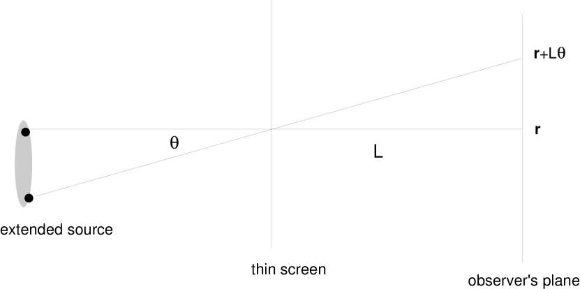
Figure 2: The geometry of the scattering assumed in calculating the effect of a source’s structure on its scintillation pattern.

Figure 2 shows that the wavefront incident on the screen at an angle ` to the line of sight, and heading towards the point ${\bf r}+L{\hbox{\boldfont\char 18\relax }}$, intersects a thin scattering screen at the same point as a normally incident wavefront, heading towards ${\bf r}$. Each of these wavefronts experiences identical scattering, and the amplification caused by the scattering screen is thus identical for these two wavefronts. It follows that scintillation pattern of an extended source is (Little & Hewish 1966),

$$\delta S_{X}({\bf r})=\int d^{2}{\hbox{\boldfont\char 18\relax }}\,b_{X}({\hbox{\boldfont\char 18\relax }})\delta I_{\rm pt}({\bf r}-L{\hbox{\boldfont\char 18\relax }}),$$ (3-22)

where $\delta S_{X}=(S_{X}-\langle S_{X}\rangle)/\langle S_{X}\rangle$ is the fractional flux density deviation in Stokes parameter $X=[I,Q,U,V]$, and $b_{X}({\hbox{\boldfont\char 18\relax }})$ is the angular brightness distribution of the source as observed at the scattering screen, normalized such that $\int b_{I}({\hbox{\boldfont\char 18\relax }})d^{2}{\hbox{\boldfont\char 18\relax }}=1$ and $\int b_{Y}({\hbox{\boldfont\char 18\relax }})d^{2}{\hbox{\boldfont\char 18\relax }}=Y/I_{0},\,\,Y=[Q,U,V]$. The brightness distributions $b_{Q}$ and $b_{U}$ at the screen differ from their distributions at the source if Galactic Faraday rotation is important. The distributions at the source are found by determining the Faraday rotation along the line of sight to the source. A magnetized ISM may also induce fluctuations in the amount of radiation transferred between Stokes $Q$, $U$ and $V$, however the fluctuations in the degree of birefringence are of order $\Omega_{e}/\omega_{p}\sim 10^{-8}$ smaller than the phase fluctuations considered here, and are probably unimportant for the scattering considered here (see Macquart & Melrose 2000).

The flux density deviations observed in an extended source are connected to the scintillation statistics of a point source by

$$C_{XY}({\bf r}) = \langle\delta S_{X}({\bf r}^{\prime})\delta S_{Y}({\bf r}+{\bf r}^{\prime})\rangle$$ (3-23)

$$= \int d^{2}{\hbox{\boldfont\char 18\relax }}d^{2}{\hbox{\boldfont\char 18\relax }}^{\prime}b_{X}({\hbox{\boldfont\char 18\relax }})b_{Y}({\hbox{\boldfont\char 18\relax }}^{\prime})\langle\delta I_{\rm pt}({\bf r}^{\prime}-L{\hbox{\boldfont\char 18\relax }})\delta I_{\rm pt}({\bf r}^{\prime}+{\bf r}-L{\hbox{\boldfont\char 18\relax }}^{\prime})\rangle.$$

The Fourier-transformed equivalent of equation (3-23) illustrates clearly the connection between source structure and the scintillation statistics via the power spectrum of intensity fluctuations,

$$W_{XY}({\bf q})=\widetilde{C_{XY}}({\bf q}) = \langle\widetilde{S}_{X}({\bf q})\widetilde{S}_{Y}^{*}({\bf q})\rangle$$ (3-24)

$$= \frac{1}{L^{4}}[\widetilde{B}_{X}({\bf q})\widetilde{B}_{Y}^{*}({\bf q}){W_{II}}_{\rm pt}({\bf q})],$$

where $B_{X}({\hbox{\boldfont\char 18\relax }})=b_{X}({\hbox{\boldfont\char 18\relax }}/L)$, the Fourier transform of a function is denoted with a tilde, and we have made use of equation (3-4). The quantity $B_{X}(\hbox{\boldfont\char 18\relax })$ is identical to the visibility $\Gamma_{X}(0;{\bf r})$ of the previous section. Equation (3-24) may be inverted to derive information on the structure of a scintillating source if the scattering properties of the ISM, embodied in ${W_{II}}_{\rm pt}({\bf q})$, are known.

Equation (3-24) may be interpreted as follows. The quantity ${W_{II}}_{\rm pt}({\bf q})$ is the power spectrum of intensity fluctuations in the scintillation pattern that would be observed for a point source. The quantity $\widetilde{B}_{X}({\bf q})\widetilde{B}_{Y}^{*}({\bf q})$ is the power spectrum of intensity structure in the source. The resultant power spectrum of intensity fluctuations, $\widetilde{C_{XY}}({\bf q})$, is that of a point source if the angular structure contained in source is smaller than the scale of the scintillation pattern for a point source (ie. the source is unresolved by the ISM). On the other hand, the observed scintillation pattern is dominated by source angular structure if the source is larger than the scale of the scintillation pattern for a point source. For example, scintillations in the weak scattering regime contain power on length scales $r\gtrsim r_{\rm F}$ (equivalent to $q\lesssim 1/r_{\rm F}$). Source structure has no measurable effect if the source angular size is less than the angular scale of the scintillation pattern (ie. when $\theta_{S}<r_{\rm F}/D$).

If the angular size of the source is smaller than the scale size of the scintillation pattern for a point source, the term in square brackets in (3-24) is approximated by ${W_{II}}_{\rm pt}({\bf q})$. This is because ${W_{II}}_{\rm pt}({\bf q})$ decreases much faster with $q$ than $\widetilde{B_{I}}({\bf q})\widetilde{B_{I}}^{*}({\bf q})$. On the other hand, if the source angular size exceeds that of the scintillation pattern for a point source, we can use the approximation ${W_{II}}_{\rm pt}\approx 2.8\,q^{4-\beta}r_{\rm F}^{4}/r_{\rm diff}^{\beta-2}$ for small $q$ to obtain (see equation (3-23))

$$C_{XY}({\bf r})\approx\frac{2.8\,r_{\rm F}^{4}r_{\rm diff}^{2-\beta}}{(2\pi)^{2}L^{4}}\int d^{2}{\bf q}\,e^{-i{\bf q}\cdot{\bf r}}q^{4-\beta}\tilde{B_{X}}({\bf q})\tilde{B_{Y}}^{*}({\bf q}).$$ (3-25)

Sources sufficiently large to be resolved by the scattering medium exhibit smaller and slower intensity fluctuations relative to unresolved sources. The intensity modulation index, $C_{XY}(0)$, of an resolved source is therefore smaller than that of an unresolved source. This is evident from equation (3-24). The amplitude of $C_{XY}(0)$ decreases if the terms due to the source cut off $C_{XY}({\bf q})$ before ${W_{II}}_{\rm pt}$ reaches its maximum value (e.g. at $q\sim 1/r_{\rm F}$ for weak scattering).

4 Earth Orbit Synthesis

The earth’s orbital motion allows the scintillation pattern of a scattered source to be mapped in two dimensions. This is because the velocity of an earth-based observer relative to the ISM changes as the earth’s orbital velocity changes during the course of a year. An observer moving at a velocity ${\bf v}$ relative to the ISM samples the scintillation pattern along the direction parallel to ${\bf v}$. It is possible to measure the correlations $\Gamma_{X}({\bf r}={\bf v}t)$ or $C_{XY}({\bf r}={\bf v}t)$ for observations a time $t$ apart. The quantity $\Gamma_{X}({\bf r})$ can be measured over short coherent integrations (see, e.g. Goodman & Narayan 1989). A good approximation to the quantity $C_{XY}({\bf r})$ can typically be derived from observations of $\gtrsim 5$ scintles, typically requiring one to two days flux density monitoring for typical IDV sources.

Over the course of the year observations at different epochs sample the scintillation pattern in different directions, as the velocity of the earth changes around the solar circle. In particular, if the velocity of the ISM is comparable to the earth’s, then a strong “annual cycle” effect will appear in the observed IDV pattern, as has been observed already in J1819+3845 (Dennett-Thorpe & de Bruyn 2001a) and 0917+624 (Jauncey & Macquart 2001; Rickett et al. 2001). This enables measurement of $\Gamma_{X}({\bf r})$ or $C_{XY}({\bf r})$ for a large range of orientations of ${\bf r}$, and the information may be inverted to obtain source structure provided that it is stable on a timescale long enough for it to be mapped. The main limitation to the technique is that one does not always know ${\bf v}$ because the velocity of the ISM is not generally known. Thus one must solve simultaneously for ${\bf v}$ and the source structure, or measure ${\bf v}$ directly from observations of the time delay between the scintillation pattern as observed at two widely separated ($\gtrsim 3000$ km) receivers as the scintillation pattern passes across the earth (Jauncey et al. 2001, Dennett-Thorpe & de Bruyn 2002).

We demonstrate the technique with several examples, concentrating on Earth Orbit Synthesis using intensity fluctuations.

4.1 An example using Intensity Fluctuations

An intensity image of the structure in a scintillating source requires measurement of the autocorrelation function $C_{II}({\bf r})$. It is not possible to measure the spatial structure of the scintillation pattern of a source, $C_{II}({\bf r})$, directly. The scale of the scintillation pattern is usually larger than that of earth so that it is impossible to measure $C_{II}({\bf r})$ on sufficiently long baselines ${\bf r}$. This problem is overcome by measuring the correlations of the scintillation signal as a function of time, rather than baseline. One measures the temporal correlation function

$${C_{II}}_{t}(t)=\frac{\langle I(t^{\prime})I(t+t^{\prime})\rangle}{\langle I\rangle^{2}}-1.$$ (4-1)

The correlation between two scintillation signals measured a time $t$ apart at the same receiver may be derived from the correlation in the scintillation pattern measured by two receivers a distance ${\bf r}$ apart. The relation between the temporal and spatial intensity autocorrelation functions is thus

$${C_{II}}_{t}(t)=C_{II}({\bf r}={\bf v}t)=\frac{1}{(2\pi)^{2}\,L^{4}}\int d^{2}{\bf q}\,e^{-i{\bf q}\cdot{\bf r}}\left[\widetilde{B_{I}}({\bf q})\widetilde{B_{I}}^{*}({\bf q}){W_{II}}_{\rm pt}({\bf q})\right].$$ (4-2)

An important point in connection with (4-2) is that the modulation depth of the scintillation pattern, $C_{II}(0)$ is independent of the velocity of the scattering medium relative to earth. For instance, the depth of the intensity modulations does not depend on whether the scintillation pattern moves parallel or orthogonal to the long axis of an elongated source. However, we see that the characteristic timescale of the scintillations depends strongly on the direction of motion if ${\bf v}$ varies during the course of a year.

The effect of source structure is particularly simple when a source undergoes weak scattering and its angular size is larger than that of the scintillation pattern of a point source (ie. $\theta_{S}>r_{\rm F}/D$). Equation (3-25) is applicable in this case, and we assume $\beta=4$ instead of the usual Kolmogorov value of $\beta=11/3$ to simplify the algebra and derive analytic results. We obtain

$$C_{II}({\bf r})=\frac{2.8\,r_{\rm F}^{4}}{r_{\rm diff}^{2}L^{4}}\int d^{2}{\bf q}\,e^{i{\bf q}\cdot{\bf r}}\,|\widetilde{B_{I}}({\bf q})|^{2},\qquad L\theta_{S}>r_{\rm F}.$$ (4-3)

This expression, and the assumptions made in deriving it, are employed in the following examples.

4.1.1 Elongated source

We illustrate Earth Orbit Synthesis by examining the combined effect of source structure and velocity variations on a source with elliptical brightness distribution:

$$b_{I}({\hbox{\boldfont\char 18\relax }})=\frac{1}{\alpha_{x}\alpha_{y}\pi}\exp\left[-\left(\frac{\theta_{x}}{\alpha_{x}}\right)^{2}-\left(\frac{\theta_{y}}{\alpha_{y}}\right)^{2}\right],$$ (4-4)

where $\alpha_{x}$ and $\alpha_{y}$ are chosen to be the source angular scales parallel to the ${\bf e}_{\parallel}$ and ${\bf e}_{\perp}$ axes respectively. This choice is made for convenience only, and it is simple to re-orient the source at an angle $\xi$ to the axes by making the transformation $(x,y)\rightarrow(x\cos\xi+y\sin\xi,-x\sin\xi+y\cos\xi)$. Combining equations (4-3) and (4-4) yields the following intensity autocorrelation function

$$C_{II}({\bf r})=\frac{2.8\,r_{\rm F}^{4}}{2\pi\alpha_{x}\alpha_{y}L^{2}r_{\rm diff}^{2}}\exp\left[-\left(\frac{x^{2}}{2L^{2}\alpha_{x}^{2}}+\frac{y^{2}}{2L^{2}\alpha_{y}^{2}}\right)\right],\qquad L\alpha_{x,y}>r_{\rm F}$$ (4-5)

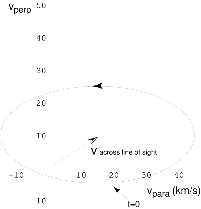
Figure 3: The scintillation speed of a source located at ecliptic co-ordinates $(\theta,\phi)=(30^{\circ},0^{\circ})$ with an intrinsic ISM velocity of $(V_{\parallel},V_{\perp})=(15,10)$ km/s.

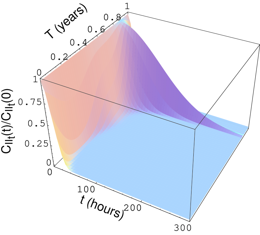
Figure 4: The observed intensity autocorrelation function as a function of time and a epoch for an elliptical source whose angular size exceeds scattering disk and with a brightness distribution given by equation (4-4) with $L\,\alpha_{x}=10^{9}$ m and $L\,\alpha_{y}=10^{9}$ m. Panel (a) shows the evolution of the temporal autocorellation function, ${C_{II}}_{t}$ throughout the year in the limit $\beta\rightarrow 4$, while (b) shows the evolution of the decorrelation timescale.

It is possible to determine the temporal decorrelation of the scintillation signal, for a given scintillation speed and direction. In the following we use $V_{\parallel}=15$ km/s, $V_{\perp}=10$ km/s and we assume the source has ecliptic co-ordinates $\theta=30^{\circ}$ and $\phi=0$. The variation in the scintillation speed over the course of a year is shown in Fig. 3. Figures 4(a) and 5(a) show how the intensity temporal autocorrelation function $C_{II}(t)$ varies throughout the year for an elliptical source with these screen parameters.

The effect of source structure is evident in the timescale of variability. It is convenient to define the decorrelation timescale, $t_{\rm dc}$ as the time in which the intensity correlation falls to $1/e$ of its maximum value. The decorrelation timescale for the elliptical source described by equation (4-5) is

$$t_{\rm dc}=\left[\frac{({\bf v}_{\rm scint}\cdot{\bf e}_{\parallel})^{2}}{2L^{2}\alpha_{x}^{2}}+\frac{({\bf v}_{\rm scint}\cdot{\bf e}_{\perp})^{2}}{2L^{2}\alpha_{y}^{2}}\right]^{-1/2}.$$ (4-6)

Changes in the magnitude of ${\bf v}_{\rm scint}$ cause changes in the scintillation timescale even if the source is circularly symmetric, whereas changes in the direction of ${\bf v}_{\rm scint}$ only result in changes in $t_{\rm ISS}$ if the source is elongated, when $\alpha_{x}\neq\alpha_{y}$.

Figures 4(b) and 5(b) plot the variation in decorrelation timescale as a function of epoch for a specific scintillation velocity for the elliptical source with two different source parameters, $L\,\alpha_{x}=10^{9}$ m and $L\,\alpha_{y}=10^{9}$ m and $5\times 10^{9}$ m respectively. Fig. 4(b) shows the expected scintillation timescale for a circularly symmetric source, and Fig. 5(b) the timescale for an elongated source. The peak in the scintillation timescale at $T\approx 0.9$ yr is common to both plots and occurs because the scintillation speed reaches a minimum. The emergence of another peak in Fig. 5(b) occurs due to the presence of structure in the source, here an elongation along the $y$-axis. The peak occurs at the time of the year that the scintillation direction is tangential to the long axis of the source.

4.1.2 Two-component source

A source with two components shows richer structure in the statistics of the intensity variations. We consider two gaussian patches of emission, the central peak having an intensity $a_{0}I_{0}$ ($0<a_{0}<1$) and the other, located at an angular separation of ${\hbox{\boldfont\char 18\relax }}_{0}$, having an intensity $(1-a_{0})I_{0}$. The two subsources have identical angular scales $\alpha$ and we again assume that the angular diameters of the subsources exceed the angular diameter of the scintillation pattern due to a point source, so that equation (3-25) applies in the regime of weak scattering. The source angular brightness distribution is

$$b_{I}({\hbox{\boldfont\char 18\relax }})=\frac{a_{0}}{\pi\alpha^{2}}\exp\left[-\frac{{\hbox{\boldfont\char 18\relax }}^{2}}{\alpha^{2}}\right]+\frac{1-a_{0}}{\pi\alpha^{2}}\exp\left[-\frac{({\hbox{\boldfont\char 18\relax }}-{\hbox{\boldfont\char 18\relax }}_{0})^{2}}{\alpha^{2}}\right],$$ (4-7)

for which the resulting spatial intensity autocorrelation function is

$$C_{II}({\bf r})=\frac{r_{\rm F}^{4}}{4\alpha^{2}L^{2}\pi^{2}r_{\rm diff}^{2}}\exp\left[-\frac{r^{2}+L^{2}{\hbox{\boldfont\char 18\relax }}_{0}^{2}}{2\alpha^{2}L^{2}}\right]\left((1-2a_{0}+2a_{0}^{2})\exp\left[\frac{{\hbox{\boldfont\char 18\relax }}_{0}^{2}}{2\alpha^{2}}\right]+2a_{0}(1-a_{0})\cosh\left[\frac{{\bf r}\cdot{\hbox{\boldfont\char 18\relax }}_{0}}{\alpha^{2}L}\right]\right).$$ (4-8)

Figure 6 plots the spatial intensity autocorrelation function of this source. This function has three peaks. The lightcurve of a two-component source therefore exhibits interesting behaviour when the scintillation direction is parallel to the line joining the two substructures. An observer then measures the spatial autocorrelation function along a line that joins the three peaks in the autocorrelation function.

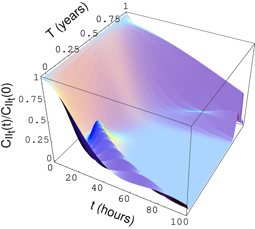
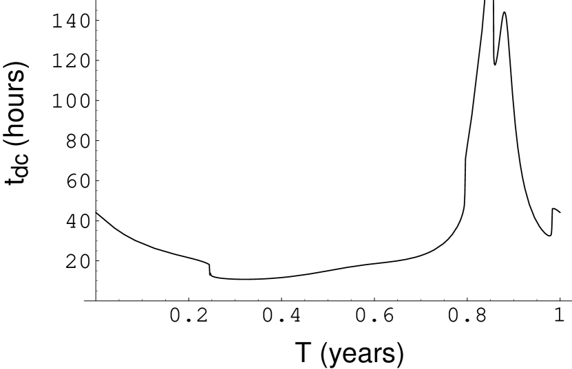
Figure 7: The observed intensity autocorrelation function as a function of time and a epoch for a source whose angular size exceeds scattering disk and with a brightness distribution given by equation (4-4) with $\alpha_{x}=4\times 10^{9}$, $\alpha_{y}=10^{9}$ and $a_{0}=0.5$. Panel (a) shows the evolution of the temporal autocorellation function, ${C_{II}}_{t}$ throughout the year ($\beta\rightarrow 4$), while (b) shows the evolution of the decorrelation timescale.

A specific example of such behaviour is illustrated in Figure 7, which demonstrates how the temporal autocorrelation function of a two component source changes throughout the course of a year. At $T\approx 0.0-0.2$ yr the scintillation velocity is parallel to the direction of the two separated peaks, and a second bump is visible in the temporal intensity autocorrelation function.

4.1.3 Polarization reference mapping

Only limited information about source structure is available from Earth Revolution Synthesis using intensity fluctuations. It is impossible to determine $b_{I}(\hbox{\boldfont\char 18\relax })$ directly from $C_{II}({\bf r})$. Only the correlation of the angular brightness distribution, $\langle b_{I}(\hbox{\boldfont\char 18\relax }+\hbox{\boldfont\char 18\relax }^{\prime})b_{I}(\hbox{\boldfont\char 18\relax }^{\prime})\rangle$, can be derived.

However, Earth Orbit Synthesis is useful even when the brightness distribution $b_{I}({\hbox{\boldfont\char 18\relax }})$ cannot be ascertained exactly. IDV sources often exhibit fluctuations in Stokes $Q$, $U$ and $V$ that are dissimilar to those observed in $I$. This occurs if the polarized structure of the source differs from its structure in total intensity. This substructure can be mapped relative to the total intensity structure, using the correlations $C_{IQ}({\bf r})$, $C_{IU}({\bf r})$ and $C_{IV}({\bf r})$ to find the quantities $\langle b_{I}({\hbox{\boldfont\char 18\relax }^{\prime}+\hbox{\boldfont\char 18\relax }})b_{Q}({\hbox{\boldfont\char 18\relax }^{\prime}})\rangle$, etc.. It is thus possible to map the brightness distribution of a source in one Stokes parameter relative to another Stokes parameter, as has been shown for both the linear and circular polarized components in PKS 1519$-$273 (Macquart et al. 2000).

5 Conclusion

Measurement of the scintillation characteristics of IDV sources allows their structure to be investigated with microarcsecond resolution. The radio structures of IDV sources are currently of interest because of their high brightness temperatures. Earth Orbit Synthesis has the potential to determine the origin of these compact structures; it can determine, for example, whether the observed emission emanates from the central cores of these objects or from the bases of jets.

Short timescale polarization variability in IDV sources indicates the presence of polarization structure on similarly fine scales and — in many cases — on even smaller scales than the structure in total intensity. The advantage of Earth Orbit Synthesis over traditional polarimetric imaging is its high resolution. Such a high resolution probe is less subject to beam-depolarization. Indeed, this mapping technique is already discovering remarkable detail about the polarized sub-structure of IDV sources (e.g. Macquart et al. 2000).

The observed two-dimensional scintillation pattern of a scattered radio source is highly influenced by source structure. This pattern can be measured in two dimensions if the apparent velocity of the scintillation across the line of sight to a scattered source changes; changes in direction allow an observer to probe source structure along different directions. Direction changes occur when the velocity of the scattering material is comparable to the earth’s velocity, and the vector sum of these two velocities changes during the course of a year.

The derivation of source structure requires measurement of the scintillation fluctuations at several epochs over the course of a year. This is achieved by measuring the temporal decorrelation of the intensity $\langle I(t)I(t+t^{\prime})\rangle$. Many IDV sources also exhibit polarization variability, which is often not well correlated with the total intensity. This occurs when the source structure in polarized and total intensity emission differs. Polarized substructure information is available by measuring the temporal cross-correlations $\langle X(t)Y(t+t^{\prime})\rangle$ between Stokes parameters $X$ and $Y$. It is possible to measure the polarized substructure of a source with reference to the intensity emission to high precision.

An advantage of the Earth Orbit Synthesis technique is the capability to compare source structure between frequencies. For example, one could compare the angular separation between source components as a function to yield information relating to opacity changes with frequency. Analysis of the data on PKS 1519$-$273 (Macquart et al. 2000) demonstrates not only the power to compare source structure at two frequencies, but even to compare the relative source properties in different Stokes parameters.

It should be emphasised that the use of Earth Orbit Synthesis as an imaging technique is subject to limitations. Firstly, the scintillation process only probes source structure over a limited angular size range. Consequently, while Earth Orbit Synthesis probes microarcsecond structures, it provides no information on the relation between microarcsecond and larger scale structure. Secondly, the use of autocorrelation functions in the imaging process is a necessary but severe limitation to any imaging that can be achieved. This technique yields the power spectrum of the source brightness distribution and, as such discards phase information that is present in normal rotational synthesis. The stochastic nature of the scintillation process forces us to use ensemble average quantities such as autocorrelation functions.

The angular resolution achievable using scintillation-based imaging depends on the properties of the scattering medium. In the regime of weak scattering, generally applicable at frequencies $\nu\gtrsim 5$ GHz, the intensity scintillations are sensitive to angular scales $\theta\sim r_{\rm F}/D\propto\nu^{-1/2}$. The scattering is strong at frequencies $\nu\lesssim 5$ GHz. The refractive scintillation exhibited by IDV sources in this regime is less sensitive to small angular scales because the angular resolution achievable is $\theta\sim r_{\rm ref}/D$ which is large, and scales as $\nu^{-2.2}$ for a Kolomogorov spectrum of inhomogeneities. Strong scattering is typically sensitive to sizes $\gtrsim 0.1$ mas, and hence can be found in many more flat-spectrum sources, particularly at low Galactic latitudes. Thus, while less useful competing against VLBI for milliarcsecond imaging, strong scattering here remains an excellent probe of the ISM close to the Galactic plane.

A program to use Earth Orbit Synthesis to map structure in IDV sources is currently underway using the Australia Telescope Compact Array (Bignall et al. 2001).

Figure 5: The observed intensity autocorrelation function as a function of time and a epoch for a source whose angular size exceeds scattering disk and with a brightness distribution given by equation (4-4) with $L\,\alpha_{x}=10^{9}$ m and $L\,\alpha_{y}=5\times 10^{9}$ m. Panel (a) shows the evolution of the temporal autocorellation function, ${C_{II}}_{t}$ throughout the year (in the limit $\beta\rightarrow 4$), while (b) shows the evolution of the decorrelation timescale.

Figure 6: The spatial intensity autocorrelation function of a source whose angular size exceeds that of the scattering disk and with a brightness distribution given by equation (4-7) with $L\alpha=10^{9}$ m and a source separation of $L({\theta_{0}}_{x},{\theta_{0}}_{y})=(3,0)\times 10^{9}$ m, $a_{0}=0.5$ and assuming $\beta\rightarrow 4$.

References

- Armstrong et al. (1995) Armstrong, J.W., Rickett, B.J. & Spangler, S.R., 1995, ApJ, 443, 209
- Begelman et al. (1994) Begelman, M.C., Rees, M.J. & Sikora, M. 1994, ApJ, 429, L57
- Bignall et al. (2001) Bignall, H., Jauncey, D.L., Kedziora-Chudczer, L.L., Lovell, J.E.J., Macquart, J.-P., Rayner, D.P., Tingay, S.J., Tzioumis, A.K., Clay, R.W., Dodson, R.G., McCulloch, P.M. & Nicholson, G.D. 2001, to appear in the proceedings of “AGN Variability across the Electromagnetic Spectrum,” held in Sydney June 2001
- Chandran and Backer (2002) Chandran, B.D.G. & Backer, D.C. 2002, ApJ, submitted (astro-ph/0202261)
- Cornwell et al. (1989) Cornwell, T.J., Anantharamaiah, K.R. & Narayan, R., 1989, J. Opt. Soc. Am. A, 6, 977
- Dennett-Thorpe and de Bruyn (2000) Dennett-Thorpe, J., & de Bruyn, A.G. 2000, ApJ, 529, 65L
- Dennett-Thorpe and de Bruyn (2001a) Dennett-Thorpe, J. & de Bruyn, A.G. 2001a, in Proceedings of IAU 205, “Galaxies and their Constituents at the highest angular resolution,” Eds. Schilizzi, Vogel & Elvis, ASP Conf. Series, 88
- Dennett-Thorpe and de Bruyn (2002) Dennett-Thorpe, J. & de Bruyn, A.G. 2002, Nature, 415, 57
- Gochelashvily and Shishov (1975) Gochelashvily, K.S. & Shishov, V.I., 1975, Opt. Quant. Electron., 7, 524
- Goodman and Narayan (1989) Goodman, J. & Narayan, R. 1989, MNRAS, 238, 995
- Heeschen (1984) Heeschen, D.S. 1984, AJ, 89, 1111
- Jauncey et al. (2000) Jauncey, D.L., Kedziora-Chudczer, L.L., Lovell, J.E.J., Nicholson, G.D., Perley, R.A., Reynolds, J.E., Tzioumis, A.K., Wieringa, M.H. 2000, in Proceedings of the VSOP Symposium, “Astrophysical Phenomena Revealed by Space VLBI,” Eds. Hirabayashi, H., Edwards, P.G. & Murphy, D.W., 147
- Jauncey et al. (2001) Jauncey, D.L., Kedziora-Chudczer, L.L., Macquart, J.-P., Lovell, J.E.J., Perley, R.A., Nicolson, G.D., Rayner, D.P., Reynolds, J.E., Tzioumis, A.K., Wieringa, M.H. & Bignall, H.E. 2001, in Proceedings of IAU 205, “Galaxies and their Constituents at the highest angular resolution,” Eds. Schilizzi, Vogel & Elvis, ASP Conf. Series, 84
- Jauncey and Macquart (2001) Jauncey, D.L. & Macquart, J.-P. 2001, A&A, 370, L9
- Jokipii and Hollweg (1970) Jokipii, J.R. & Hollweg, J.V. 1970, ApJ, 160, 745
- Kedziora-Chudczer et al. (1997) Kedziora-Chudczer, L., Jauncey, D.L., Wieringa, M.H., Walker, M.A., Nicolson, G.D., Reynolds, J.E. & Tzioumis, A.K. 1997, ApJ, 490, L9
- Kedziora-Chudczer et al. (2000) Kedziora-Chudczer, L.L. et al. 2000, in the proceedings of IAU 182 held in Guiyang, China.
- Kedziora-Chudczer et al. (2001) Kedziora-Chudczer, L.L., Jauncey, D.L., Wieringa, M.H., Tzioumis, A.K. & Reynolds, J.E., 2001, MNRAS, 325, 1411
- Kraus et al. (1999) Kraus, A., Witzel, A., Krichbaum, T.P., Lobanov, A.P., Peng, B. & Ros, E., 1999, A&A, 352, L107
- Little and Hewish (1966) Little, L.T. & Hewish, A. 1966, MNRAS, 134, 221
- Macquart et al. (2000) Macquart, J.-P., Kedziora-Chudczer, L., Rayner, D.P., Jauncey, D.L., 2000, ApJ, 538, 623
- Macquart and Melrose (2000) Macquart, J.-P. & Melrose, D.B. 2000, ApJ, 545, 798
- Narayan (1992) Narayan, R., 1992, Phil. Trans. R. Soc. Lond. A, 341, 151
- Quirrenbach et al. (2000) Quirrenbach, A., Kraus, A., Witzel, A., Zenzus, J.A., Peng, B., Risse, M., Krichbaum, T.P., Wegner, R., Naundorf, C.E. 2000, A&AS, 141, 221.
- Rickett et al. (1995) Rickett, B.J., Quirrenbach, A., Wegner, R., Krichbaum, T.P. & Witzel, A., 1995, A&A, 293, 479
- Rickett et al. (2001) Rickett, B.J., Witzel, A., Kraus, A., Krichbaum, T.P. & Qian, S.J. 2001, ApJ, 550, L11
- Salpeter (1967) Salpeter, E.E. 1967, ApJ, 147, 434
- Walker (1998) Walker, M.A., 1998, MNRAS, 294, 307
- Witzel et al. (1986) Witzel, A., Heeschen, D. S., Schalinski, C. & Krichbaum, Th. 1986, Mitteil. Astron. Gesellschaft, 65, 239