Orbital dynamics of three-dimensional bars:
II. Investigation of the parameter space

Abstract

We investigate the orbital structure in a class of 3D models of barred galaxies. We consider different values of the pattern speed, of the strength of the bar and of the parameters of the central bulge of the galactic model. The morphology of the stable orbits in the bar region is associated with the degree of folding of the x1-characteristic. This folding is larger for lower values of the pattern speed. The elongation of rectangular-like orbits belonging to x1 and to x1-originated families depends mainly on the pattern speed. The detailed investigation of the trees of bifurcating families in the various models shows that major building blocks of 3D bars can be supplied by families initially introduced as unstable in the system, but becoming stable at another energy interval. In some models without radial and vertical 2:1 resonances we find, except for the x1 and x1-originated families, also families related to the z-axis orbits, which support the bar. Bifurcations of the x2 family can build a secondary 3D bar along the minor axis of the main bar. This is favoured in the slow rotating bar case.

1 Introduction

Barred galaxies have bars of very different strength, ranging from the weak bars of SAB galaxies to the strong bars of e.g. NGC 1365 [Lindblad 1999]. They may have large, small, or no bulge components in their centers. The possibility that bars in late-type barred spiral galaxies end at their inner Lindblad resonance (hearafter ILR) has also been considered (Lynden-Bell 1979, Combes & Elmegreen 1993, Polyachenko & Polyachenko 1994) and this would imply that in some cases bars may have corotation far beyond their ends. It is thus important to understand whether and to what extent the orbital structure changes with the basic parameters in the models. We investigate this here using a class of models, the individual representatives of which differ in their central mass concentration and in the pattern speed and strength of the bar.

We follow the evolution of all the families of periodic orbits we think may play a role in the dynamics and morphology of bars and peanuts. We believe we indeed have all the main families for two reasons. First, the edge-on profiles of the galaxies are mainly affected by the vertical bifurcations up to the 4:1 vertical resonance. Beyond this resonance the orbits of the bifurcating 3D families remain close to the equatorial plane and thus do not characterize the edge-on morphology. Second, families bifurcated at the n:1 radial resonances for $n>4$ do not in general support the bar (e.g. Contopoulos & Grosbøl 1989, Athanassoula 1992).

The models presented here are static, but they may be viewed as corresponding to individual phases of an evolutionary process of the dynamical evolution of a galaxy within a Hubble time. Therefore, a complete investigation of the dynamical system is necessary in order to find all orbits possibly associated with the presence of specific morphological features.

In the first paper of this series (Skokos, Patsis & Athanassoula 2002, hereafter paper I) we presented the basic families in a model composed of a Miyamoto disc of length scales A=3 and B=1, a Plummer sphere of scale length 0.4 for a bulge and a Ferrers bar of index 2 and axial ratio $a:b:c=6:1.5:0.6$. The masses of the three components satisfy $G(M_{D}+M_{S}+M_{B})=1$ and are given in Table 1. The length unit is 1 kpc, the time unit 1 Myr and the mass unit $2\times 10^{11}M_{\odot}$.

In the present paper we compare the orbital structure of our basic model with those encountered in five more models. Our models, including the fiducial model A1 of paper I, are described in Table 1. G is the gravitational constant, M_D, M_B, M_S are the masses of the disk, the bar and the bulge respectively, $\epsilon_{s}$ is the scale length of the bulge, $\Omega$_b is the pattern speed of the bar, $E_{j}$(r-IILR) and $E_{j}$(v-ILR) are the values of the Jacobian for the inner radial ILR and the vertical 2:1 resonance respectively, and $R_{c}$ is the corotation radius.

Table 1: Parameters of our models. G is the gravitational constant, M_D, M_B, M_S are the masses of the disk, the bar and the bulge respectively, $\epsilon_{s}$ is the scale length of the bulge, $\Omega$_b is the pattern speed of the bar, $E_{j}$(r-IILR) is the Jacobian for the inner radial ILR, $E_{j}$(v-ILR) is the Jacobian for the vertical 2:1 resonance, $R_{c}$ is the corotation radius. The comment in the last column characterizes the model in order to facilitate its identification.

model name	GMD	GMB	GMS	$\epsilon_{s}$	$\Omega$b	$E_{j}$(r-IILR)	$E_{j}$(v-ILR)	$R_{c}$	comments
A1	0.82	0.1	0.08	0.4	0.0540	-0.441	-0.360	6.13	fiducial
A2	0.82	0.1	0.08	0.4	0.0200	-0.470	-0.357	13.24	slow bar
A3	0.82	0.1	0.08	0.4	0.0837	-0.390	-0.364	4.19	fast bar
B	0.90	0.1	0.00	–	0.0540	–	–	6.00	no bulge
C	0.82	0.1	0.08	1.0	0.0540	–	-0.364	6.12	extended bulge
D	0.72	0.2	0.08	0.4	0.0540	-0.467	-0.440	6.31	strong bar

This paper is organized as follows: In section 2 we discuss models with fast, or with slow bars. Section 3 introduces a model with no 2:1 resonances, section 4 a model with vertical but no radial ILR, and section 5 a model with a massive bar. We conclude in section 6.

2 The effect of pattern speed

2.1 A slow rotating bar

Model A2 is the same as model A1 in everything, except for the pattern speed, $\Omega$${}_{b}=0.02$, which is less than half that of model A1. The corotation in this model is at 13.24, rather than at 6.13 as in model A1, and the outer inner Lindblad resonance (OILR) is now at 6.1, i.e. roughly the end of the bar or the corotation distance of the models with $\Omega$_b = 0.054.

The changes in the dynamical behaviour are much more important than a stretching of the corotation radius by a factor larger than two and an enlargement of the x2-x3 loop in the characteristic and in the stability curves of the model. New bifurcations and new gaps are introduced, while the morphology of some of the existing families changes drastically. The differences are so big as to introduce nomenclature issues. Let us start our examination of the main simple-periodic families and of their bifurcations with the help of the characteristic diagram for planar orbits, shown in Fig. 1.

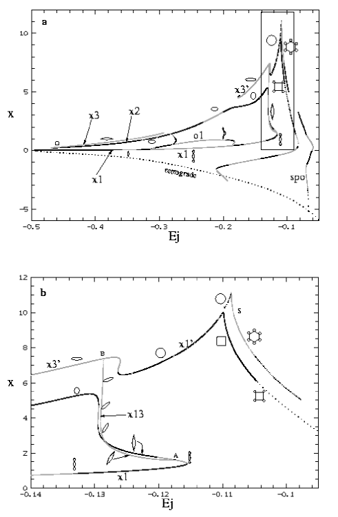
Figure 1: Characteristic diagram for the 2D families of model A2. Grey parts of the lines show the unstable parts of the families. In (b) we give an enlargement of the area included in the frame in (a).

Following the convention introduced in paper I, we draw with a black line the parts of the characteristics which correspond to stable parts of the families, while grey is associated with instability. There are two main characteristics, or rather families of characteristics. The lower one is confined to the region below $x\approx 5.5$. It is divided from the upper characteristic by a gap, occurring roughly at $E_{j}=-0.128$. There are are also a number of 3D families bifurcating from these characteristics, of which the most important ones will be described at the end of this section.

The main feature of the characteristic diagram is a continuous curve constituted by the simple-periodic 2D families x1, x2 and x3. We will follow it counter-clockwise. Starting close to $E_{j}=-0.5$ for $x=0$ we walk along the characteristic of the typical x1 family. The orbits there are elliptical-like and support the bar.

At the first S $\rightarrow$U transition of x1 the family x1v1 is bifurcated. That means we have reached at this energy the vertical 2:1 resonance. It has a similar evolution as in the fiducial case (paper I), but it is complex unstable for a considerably smaller energy range. This affects strongly the vertical profile of the model (Patsis, Skokos & Athanassoula, 2002a hereafter paper III). Since it is a 3D family it is not included in Fig. 1.

The first radial bifurcation occurs at $E_{j}\approx-0.31$ and gives the family o1. This is stable for a tiny $E_{j}$ interval, just after the S$\rightarrow$U transition. It then follows a S$\rightarrow$U$\rightarrow$S$\rightarrow$U sequence and ends again on x1. Thus this family builds a bubble, both in the characteristic and the stability diagram, together with x1 or with its indices, as did family t1 in model A1. Its morphology, however, shows that it is related to a radial 1:1 resonance [Papayannopoulos & Petrou 1983], since both cuts with the $y=0$ axis are for $x>0$ (alternatively $x<0$), so that it can be viewed as a distorted circle. It nevertheless has three tips or ‘corners’, of which the two close to the $y$ axis are very sharp and for large $E_{j}$ values they develop loops. This morphological evolution is reflected by the small orbits drawn close to the o1 curve on Fig. 1a.

The next S$\rightarrow$U transition brings in the system x1v3. This is a 3D family, so again it is not included in the diagram. When x1 becomes again stable close to $E_{j}\approx-0.134$, its orbits have developed loops along the major axes of the ellipses. Since we are already at the area included in the frame in Fig. 1a, it is easier to follow the evolution of the families on the characteristic in Fig. 1b. We observe that close to $E_{j}=-0.115$ the curve has a bend and continues towards lower $E_{j}$ and higher $x$ values. On the bend x1 orbits are still very elongated with loops at the $y$ axis, as noted by a x1 orbit drawn there. The x1 family has developed these loops well before the bend. Between $E_{j}=-0.115$ and $E_{j}=-0.13$, at the rising part of the characteristic, towards lower $E_{j}$ values, the x1 orbits become again ellipse-like and their loops vanish (for the time being we forget about the gray branch we observe at the same area). Meanwhile, the characteristic curve has two more bends at $x$ roughly 3 and 5 respectively and for almost the same value of $E_{j}\approx-0.13$, and then follows the long branch towards lower $E_{j}$ values, which reaches $E_{j}\approx-0.47$. On this branch and close to $E_{j}=-0.13$ the x1 orbits have small ellipticities and become even rounder as we move to lower $E_{j}$ values. Finally after $E_{j}\approx-0.17$ the orbits are elongated along the minor axis of the bar, and are stable (except for $-0.23<E_{j}<-0.2$), i.e. they belong to the x2 family. At $E_{j}\approx-0.47$ the curve folds again and continues its journey towards larger $E_{j}$ values. The orbits at this branch are typical x3 orbits and exist until $E_{j}\approx-0.29$, where they change multiplicity. Thus in this model the x2 and the x3 families are continuations of the x1, the transition being made by circular and circular-like orbits, rather than by a gap as in the standard cases (Contopoulos & Grosbøl 1989, Athanassoula 1992a, paper I etc.).

At $E_{j}\approx-0.23$ the stability index associated with the 3D bifurcations intersects the $-2$ axis. So we have the bifurcation of a new family with the same multiplicity. We call this family x2v1. We emphasize the fact that this is a simple periodic family, since in model A1 (paper I) we had already encountered a 3D bifurcation of x2 (family x2mul2), which, however, is of multiplicity 2. Since this new family is a direct bifurcation of x2 at the S$\rightarrow$U transition close to $E_{j}=-0.23$, as we move towards larger values of $E_{j}$, it inherits the stability of the parent family, i.e. it is stable.

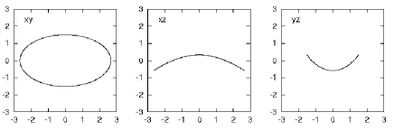
Figure 2: Stable orbit of the x2v1 family.

It stays stable for a large energy interval, $-0.23<E_{j}<-0.18$, which means that it is a family that can affect the morphology of the galaxy. Its morphology can be seen in Fig. 2. As we can see this family can support a peanut-like feature, which, however, is elongated not along the major but along the minor axis of the main bar. If such orbits are populated in a real galaxy, then they will support a 3D stellar inner bar with a ‘x2 orientation’.

Close to the part of the x1 characteristic for $-0.13<E_{j}<-0.115$, where the curve folds and extends towards lower energies (Fig. 1b), we have, besides the ‘x1 part’, a gray branch (unstable orbits) that bridges the main loop with another branch of the characteristic diagram existing at the same energies and for larger $x$ values. If this bridge was missing then we would have a classical type 2 gap as at the radial 4:1 resonance regions (Contopoulos & Grosbøl 1989). What we have now could be called a pseudo-gap. The orbits of this branch are unstable and belong to a family we call x13, since it starts for low $x$ values as x1 at point ‘A’ (Fig. 1b) and reaches at ‘B’ a horizontal branch, which is the characteristic curve of a x3-like family. x13 is a radial bifurcation in $\dot{x}$, so the curve we give in Fig. 1 for this family is just the projection of its characteristic in the ($E_{j}$,$x$) plane. The morphology of these orbits is expected to be related with inclined ellipses, whose major axis shifts from being parallel to the bar major axis (for members on or near the major loop characteristic) to parallel to the bar minor axis (for members on or near the x3^′ characteristic). The shift happens in a small energy interval, in which the x1 orbits have the longest projections on the $y$ axis. Successive orbits of x13, as we move from ‘A’ to ‘B’ (Fig. 1b), are given in Fig. 3. The evolution of the stability indices

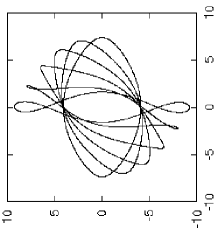
Figure 3: Successive x13 orbits. They are all unstable.

of x1 in this area follow every possible complication one could imagine in order to avoid bifurcating a stable family with similar morphology. Due to this ‘conspiracy’ it was not possible for us to find a stable x13-like family.

The second part of the characteristic diagram, at the same energies as the ‘x1 part’ and for higher $x$ values, has orbits which are x3-like. These orbits are ellipses elongated along the minor axis of the bar and are almost everywhere unstable, except for a tiny part of the characteristic for $E_{j}\approx-0.175$. We thus called them x3^′. Moving along the x3^′ branch of the characteristic towards larger $E_{j}$ values, we encounter a step-like feature in the curve (Fig. 1b) and beyond it we have planar orbits, which can be easily described as prograde quasi-circular orbits. Their general dynamical properties and their relation with other families at the area resemble those of the x1 family. So this family is a kind of continuation of x1, which we call x1^′ (as we called, for lower energies, the continuation of the x3 family x3^′). The stability indices of x1^′ oscillate and at the tangencies with the $b=-2$ axis the 3D families x1^′v4, x1^′v5 etc. are born. We call them like this because their morphology on the $(x,z)$ and $(y,z)$ projections resembles the morphology of the x1v4 and x1v5 families of the fiducial case. The bifurcated 3D families remain as stable close to the equatorial plane, i.e. they do not characterize the vertical profile of the model, although they have large stable parts. It is important to note that in this case the shape of the x1^′ orbits – and of the $(x,y)$ projections of x1^′v4 and x1^′v5 as well – are not elongated along the major axis of the bar, but are quasi-circular. Thus, they do not enhance the bar towards the corotation radius (13 kpc). This can be seen in Fig. 4.

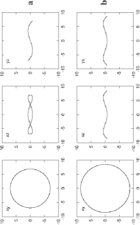
Figure 4: Stable orbits of the families x1^′v4 (a), and x1^′v5 (b).

The characteristic of x1^′, as in the case of model A1 for x1, has a local maximum at $E_{j}\approx-0.11$. At the decreasing branch (lower $x$’s for larger $E_{j}$ values) the orbits of the family develop ‘corners’. The usually rectangular-like orbits found in the 4:1 region (cf. Fig. 2g in paper I) are for this model square-like. x1^′ has a stable part just after the turning point, while in model A1 the decreasing branch is almost everywhere unstable. For yet larger energies, when the orbits at their four apocentra have loops, x1^′ is unstable.

As can be seen in Fig. 1b the gap at $E_{j}\approx-0.11$ is a real type 2 gap, the upper branch of which has stable circular orbits at the ‘increasing $x$’ part and unstable hexagonal orbits at the decreasing part following it at larger $E_{j}$ values. The latter are not much elongated along the $y$ axis. Due to this morphological evolution of the x1 family there are no elliptical-like orbits elongated along the $y$ axis to extend the bar towards corotation. The elongated orbits which reach the farthest out in the $y$ direction are elliptical-like orbits with loops, reaching $y\approx 9.4$, surrounded by a roundish structure reaching the corotation region (Fig. 5).

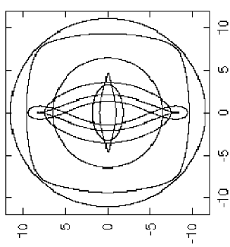
Figure 5: Stable orbits for model A2.

Before closing our description of model A2, we should mention that the family x1v4, initially bifurcated as double unstable, becomes stable for larger energies and provides the system with 3D orbits with low $\overline{|z|}$. The orbit we give in Fig. 6 has $E_{j}=-0.12$,

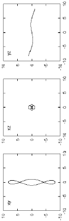
Figure 6: Stable orbit of the x1v4 family of model A2.

while the family x1v4 bifurcates for $E_{j}\approx-0.245$ at a D$\rightarrow$U transition of x1. The evolution of the stability indices of this family in model A2 is less complicated than in model A1. It nevertheless shows all kinds of instabilities we encounter in 3D Hamiltonian systems and finally ends again on x1. This means that it can be considered both as a direct and as an inverse bifurcation of x1.

Summarizing the main differences of the orbital behaviour of the slow rotating bar model from that in the fiducial case, we underline the existence of a complicated common characteristic of the x1, x2 and x3 families. As a consequence the simple-periodic families of the x1-tree appear in two parts. The second part consists of x1^′ and its 3D bifurcations. The families of the x1^′-tree have large stable parts, but they do not help the bar reach closer to corotation since they are quasi-circular (or have quasi-circular projections on the equatorial plane). The rectangular-like orbits in this case are almost squares. The model also includes a simple periodic x2-like 3D family. Other differences in the orbital behaviour from model A1 that should be mentioned is the small complex unstable part of x1v1 and the bifurcation of the family x1v4 at a D$\rightarrow$U stability transition.

2.2 A fast rotating bar

Model A3 has a fast rotating bar. Its pattern speed is 0.0837, which brings corotation to 4.2 kpc, i.e. closer to the center than the end of the imposed bar. All other parameters remain as in models A1 and A2.

The major effect, as expected, is that the OILR approaches the IILR, and the size of what we would call ‘x2-region’ is drastically reduced. In model A3 both x2 and x3 families still exist. The size of the semi-major axis of the largest x2 orbit is 0.63 kpc. This means, that the x2 orbits could support features of sizes about $\approx$ 1.2 kpc. In other words in such models, the x2 family could play a role in the dynamics of the innermost 1 kpc of the system if the corresponding orbits are populated, despite the fact that the x2-loops we find are tiny ($\Delta E_{j}\approx 0.01$) in comparison to those of models A1 and of course A2. In Fig. 7 we see the evolution of the stability indices of this model. Note the small elliptical features around $E_{j}\approx-0.385$, which are made from the combination of the stability indices of x2 and x3. The stability indices of these two families do not have any other cuts or tangencies with the $b=2$ or $b=-2$ axes and thus this model has no 3D families oriented perpendicular to bar major axis and cannot form a peanut with this orientation.

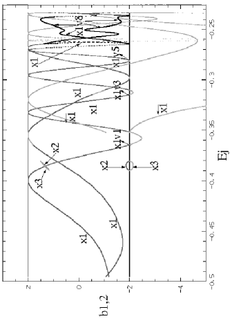
Figure 7: Stability diagram for the family x1 in model A3. The black bold curves at the right part of the figure ($-0.265<E_{j}<-0.235$) are the stability indices of the family x1v8. Light grey curves indicate instability.

The oscillations of the b1 and b2 curves of x1 bring in the system the families x1v1, x1v3 and x1v5 as stable. Their dynamical behaviour, and thus their importance for the global dynamics of the system, do not differ from what we encountered in the fiducial case, and so we do not discuss it further here. In this model x1v4 is not significant. It remains unstable until its orbits reach high $z$ values above the equatorial plane. The curves indicated by $\stackrel{{\scriptstyle\leftarrow}}{{x1}}$ correspond to the orbits at the branch of the characteristic of x1, after the bend of the curve towards lower energies for $E_{j}\approx-0.235$ (see Fig. 8 below). Light gray indicates also in Fig. 7 unstable orbits. The lower index almost goes through the point of intersection of x1 with the $-2$ axis. However, because of the location of the second index, we do not have a loop that closes on x1 there.

The new elements that the study of this model brings to the investigation of the orbital dynamics of barred potentials are focused at the region of the (type 2) gap at the 4:1 resonance. In Fig. 8 we show what is

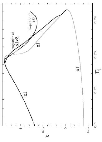
Figure 8: Part of the characteristic diagram of model A3. It shows the curve of the family x1 at the 4:1 resonance region, and the ($E_{j}$,$x$) projections of families q₀ and x1v8. Light gray color indicates unstable orbits.

new in this model on a characteristic ($E_{j}$,$x$) diagram of x1. We have also included the ($E_{j}$,$x$) projections of a planar family (q₀), which has $\dot{x_{0}}\neq 0$ in the initial conditions, and a 3D family (x1v8), which is unstable in model A1.

Let us start from the latter. As can be seen in Fig. 7, the stability index associated with the vertical bifurcations has its seventh cut with the $b=-2$ axis at $E_{j}\approx-0.265$ (the depth and size of the unstable region is very small; we observe in Fig. 7 that the depth and size of the successive unstable regions decreases with increasing energy). At this point a new stable family is born. Fig. 8 shows that this family is bifurcated just before the local maximum of the x1 characteristic curve. The $(x,z)$ and $(y,z)$ morphology of this new family is similar to that of family x1v8 of our fiducial model (cf. Fig. 17c in paper I) and thus, according to the rules set in paper I, we call it x1v8, although it emerges at the seventh vertical bifurcation. In model A3 the succession of appearance of the bifurcating families associated with the vertical 5:1 resonance is reversed compared with the families of the corresponding instability strip in the fiducial case. Now this instability strip is located before the local maximum of the x1-characteristic at $E_{j}\approx-0.26$ (Fig. 8), while in model A1 it is located beyond the corresponding local maximum. As discussed in paper I when the evolution of the stability index of x1 associated with the vertical bifurcations has successive cuts with the $b=-2$ axis giving rise to a S$\rightarrow$U$\rightarrow$S sequence in its stability, a stable and an unstable family are introduced in the system. In model A1 for all instability strips at the vertical resonances before the local maximum of the characteristic curve, the families introduced as stable at the S$\rightarrow$U transition are bifurcations in $z$, and the unstable ones, bifurcated at the U$\rightarrow$S part, are bifurcations in $\dot{z}$. The opposite is true for the 5:1 resonance instability strip located beyond the local maximum. There we had a stable family bifurcated in $\dot{z}$, which we called x1v7 and an unstable one bifurcated in $z$ we called x1v8 (paper I). In the present model the corresponding instability strip of the vertical 5:1 resonance is located before the local maximum of the x1-characteristic for $E_{j}\approx-0.26$ (Fig. 8) and the family introduced as stable is a bifurcation in $z$. Since we keep the nomenclature introduced in the fiducial model throughout this series of papers, this is family x1v8 and the bifurcation in $\dot{z}$, unstable in the present model, is x1v7.

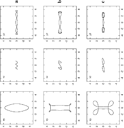
Figure 9: Orbits of the family x1v8 of model A3. From top to bottom: $E_{j}=-0.26$, $E_{j}=-0.25$ and $E_{j}=-0.24$ respectively.

We note that while the x1v7 family of model A1 very soon gets orbits with large $|z|$’s, family x1v8 is stable everywhere and its orbits remain confined close to the equatorial plane (Fig. 9).

Almost at the local maximum of the x1 characteristic, at $E_{j}\approx-0.26$, we have another S$\rightarrow$U transition of x1 (Fig. 8). There we have a radial bifurcation with ${\dot{x}}\neq 0$ . We call the resulting family q₀, since it bifurcates at the 4:1 resonance close to the local maximum, and its morphology is different than that of the q1, q2 families of model A1. Its morphological evolution, as we move along the ($E_{j}$,$x$) projection of its characteristic, is given in Fig. 10.

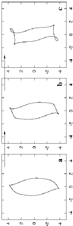
Figure 10: A sequence of three stable orbits of the q₀ family of model A3, showing its morphological evolution. They have (from left to right) $E_{j}=-0.2615,-0.260$ and $-0.255$ respectively.

In Fig. 8 we see that q0 is stable almost everywhere with only two small unstable zones. The one closer to the bifurcating point is bridged by a family (not shown in Fig. 8) existing just in this interval. The orbits of this family are slightly asymmetric with respect to the corresponding unstable orbits of q0 at the same $E_{j}$ values. Practically one could say that q0 is stable even there. The second zone of instability is in an area where the loops of q0 are big, so that the orbits are less interesting because of their morphology. Thus we conclude that practically all the morphologically interesting parts of q0 are stable.

Concluding about model A3, we can say that its differences with respect to the fiducial case are focused at the dynamics close to the local maximum of the characteristic at the radial 4:1 resonance. In general, in most other models we examined, the decreasing branches of the x1 characteristics beyond the local maximum harbor mainly unstable families. In that respect, model A3 is an exception, because at this region we can find decreasing branches with large stability regions offered not by x1 itself but by q0 and x1v8. We note that q0 and x1v8 are the most elongated rectangular-like orbits we found in any of the models we studied. In model A3 the bar is supported by the x1 and q0 families up to 3.8 kpc, with corotation at 4.2 kpc (For more details about the supported face-on morphologies of our models, see Patsis, Skokos & Athanassoula, 2002b hereafter paper IV). Further differences are the size of the x2 region, which in model A3 is very small and the insignificance of the x1v4 family. A final difference of A3 from the rest of the models we examined is the lack of a ‘bow’ structure in the stability diagrams. The rest of the orbital structure is similar to that of model A1.

3 A model without 2:1 resonances

All models presented until now include an explicit bulge component in the form of a Plummer sphere. In order to investigate the influence of central concentrations on the dynamics of the bar we consider a model without this component, and we increase the mass of the disc accordingly so that the total mass stays the same as that of the other models. This is model B, in which all other parameters are as in model A1. We note that this particular case has been studied by Pfenniger (1984).

The model is characterized by the lack of radial as well as vertical 2:1 resonances. The stability indices of x1 have their first tangency with the $b=-2$ axis at $E_{j}\approx-0.240$. We call the family bifurcated at this point x1v5 because the $(x,z)$ and $(y,z)$ projections of its orbits have the same morphology as that of the x1v5 family of model A1. x1v5 exists up to $E_{j}\approx-0.219$ where it rejoins x1. This family corresponds to the B$z_{1}$ family of Pfenniger (1984). Another 3D orbit is bifurcated from x1 at $E_{j}\approx-0.217$, and is morphologically similar to x1v5 so that we name it x1v5^′. This family has stable orbits with low $|z|$ over a reasonable energy range, i.e it is an important family of the system, as was already pointed out by Pfenniger (1984) who named it B$z_{2}$. At $E_{j}\approx-0.215$ the x1v7 family is bifurcated, which corresponds to the B$\dot{z}_{3}$ family of Pfenniger (1984). The overall evolution of the stability indices in this model is characterized by a complicated ‘bow’, around $E_{j}\approx-0.22$, reminiscent of the bow in model A1. The bow is at the center of the 3:1 region, which in this model is rather extended. The values of the indices of the 3:1 families remain smaller than 0, and all bifurcations are simple periodic families. The model has t1, t2 and 3D 3:1 orbits with t1- and t2-like projections. Its 4:1 gap is of type 2, and beyond this gap, towards corotation, the orbital behaviour resembles that of model A1.

In this model we found one more family, which has large stable parts over a very extended energy range. This family has morphological similarities with x1v4, but it is not related with the x1-tree. This means that at least as far as we have followed, it does not bifurcate from or be linked with a family belonging to the x1-tree. This family exists for $E_{j}>-0.285$ and is one of the families of periodic orbits related to the z-axis family, i.e. to the 1D orbits on the rotational axis of the system. The well known bifurcations of the z-axis family are the sao and uao families (Heisler, Merritt & Schwarzschild 1982). They are introduced at S$\rightarrow$U and U$\rightarrow$S stability transitions of the z-axis family respectively, at which we have cuts of one of the stability indices with the $b=-2$ axis. We find them considering the $z=0$ plane as a surface of section. However, if the orbits of a single periodic family are repeated $n$-times it can be considered as $n$-periodic (paper I, §2.2). As explained in Appendix I, specific values of the stability index (Eq. 8) determine the $E_{j}$ value at which an $n$-periodic family will bifurcate. These $n$-periodic families are the so called ‘deuxième genre’ families of Poincaré (1899). The family we found to be important in this model is a bifurcation of the z-axis family when we consider its orbits repeated three times, i.e. of z3, according to the nomenclature we introduced in paper I. In this case tangencies of the stability indices of z3 with the $b=-2$ axis will bifurcate two 3-periodic families and the family we discuss here is one of them. The z-axis family does not change its stability at the energies at which the new families are born. Already by studying the evolution of the stability indices of the z-axis family, we can find out from Eq. 8 the $E_{j}$ values at which 3-periodic bifurcations will appear. Thus we know that for $E_{j}=-0.285$, a bifurcation of the z-axis orbits with multiplicity 3 will be born. We call this family z3.1s and its position of birth is seen in Fig. 11.

In Fig. 11 we give the evolution of the stability indices of z3. As expected at $E_{j}\approx-0.285$ it has a tangency with the $b=-2$ axis, and z3.1s is bifurcated.

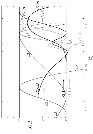
Figure 11: Part of the stability diagram of model B. It includes z3.1s, z3.1u and parts of z3.

Actually at this point two families are bifurcated. At $E_{j}\approx-0.256$ the one initially bifurcated as stable becomes unstable and remains so thereafter, while the opposite is true for the one bifurcated as unstable. We call z3.1s the one which is stable for the largest energy range and z3.1u the one initially bifurcated as stable. In any case their morphologies are very similar. We note that neither of the families have one of the stability indices on the $b=-2$ axis for some energy interval. Both stay close to it after the bifurcating point, but not on it, as one can realize by looking at the appropriate enlargement of Fig. 11 (not plotted here). The range of energies over which z3.1s is stable emphasizes its importance (Fig. 11).

The multiplicity of an orbit is associated with the surface of section we use. The z-axis orbits are calculated using as surface of section the $(x,y)$ plane, so the multiplicity in this case does not refer to the morphology of the projection of the orbit on this plane, but to the number of intersections with this plane. The detailed morphological evolution is given in Fig. 12. We observe that the multiplicity of the z3.1s family if we consider as surface of section the $y=0$ plane, as we do for all families of the x1-tree, is 1.

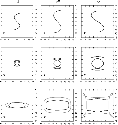
Figure 12: The morphological evolution of three stable z3.1s orbits. In (a) for $E_{j}=-0.25$, in (b) for $E_{j}=-0.22$, and in (c) for $E_{j}=-0.2$. In the $(x,y)$ projection we include, in grey, the x1 orbit with the same $E_{j}$.

In the $(x,y)$ projection we have overplotted with light grey the corresponding x1 orbits. The $(x,y)$ projection of z3.1s is always included inside the curve of the x1 orbit. It is evident that the morphology of the x1 orbits is similar but not identical to that of the z3.1s $(x,y)$ projection. We observe also that the $(x,z)$ and $(y,z)$ projections remain close to the plane of symmetry of the galactic model, at least for the lowest energies.

Apart from z3.1s, we have found other families associated with z$n$s. A case that could be mentioned is a bifurcation of z5, the shape of which is given in Fig. 13.

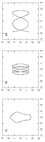
Figure 13: A stable z5.1s orbit at $E_{j}\approx-0.225$.

Orbits like this can populate a galactic bulge or the central part of disks. Indeed, although we have not an explicit bulge component in this model, our disc is not flat. Due to the geometry of the Miyamoto disc one would need in the central part orbits with projections on the $z$ axis of the order of 1 kpc in order to build a self-consistent model. Thus orbits like z5.1s should be considered. In general, however, the tangencies with the $b=-2$ axis are for larger energies and as a result, these orbits, since they are bifurcations of the z-axis, have big $\overline{|z|}$ values, and so, even if they have stable parts, are not interesting building blocks for the disc of our system.

For this model we underline the presence and importance of the z3.1s orbits and the lack of the 3D families associated with low order vertical resonances, since the first vertical bifurcation of x1 is x1v5, a family bifurcated at the vertical 4:1 resonance.

4 A model without radial ILRs

Model C is intermediate between models A1 and B. It has a Plummer sphere bulge, the scale length of which is 2.5 times larger than the scale length of the bulge of A1. It is thus considerably less centrally concentrated, and as a result its $\Omega$-$\kappa$/2 curve is less peaked. This model does not have any radial ILRs, since we have, like in model A1, $\Omega$_b=0.054.

On the other hand the model does have a vertical 2:1 resonance, where is bifurcated a x1v1 family (Fig. 14),

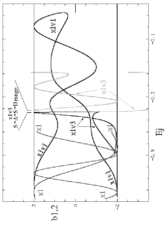
Figure 14: Stability diagram for x1, x1v1 and x1v3 in model C.

which in this model is characterized by a large stable part. After the usual S$\rightarrow$$\Delta$ transition at $E_{j}=-0.08$ the family remains always complex unstable. Furthermore, at $E_{j}=-0.26$ the maximum $z$ of the orbits is 1 kpc, and at $E_{j}$ = -0.225 the maximum $z$ is 1.5 kpc. This means that it is a very important family for the dynamics of the system. x1v3 exists as well. It has a S$\rightarrow$$\Delta$$\rightarrow$S$\rightarrow$U sequence of stability types, but the $\Delta$$\rightarrow$S$\rightarrow$U part happens in a very narrow energy range (Fig. 14). At the final S$\rightarrow$U transition the 3D family x1v3.1 depicted in Fig. 15 is bifurcated.

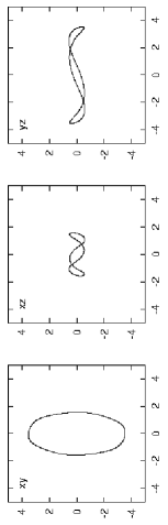
Figure 15: A stable orbit of the family x1v3.1 in model C at $E_{j}\approx-0.2235$.

In this particular model this family is just bridging x1v3 with x1v4 at $E_{j}\approx-0.2232$. At this energy x1v4 becomes stable and x1v3.1 can be considered as an inverse bifurcation of it. All this is worth mentioning because x1v3.1 is a 3D family with a $(x,y)$ projection resembling that of the family q0 of model A3.

The most important feature of model C is that x1v1 becomes complex unstable for the first time at large energies and not just after it is born as e.g. in the fiducial model A1. The consequences of this stability evolution for the global dynamics of the model are described in detail in paper III.

5 A strong bar case

Strong perturbations in Hamiltonian systems result in systems with a larger degree of orbital instabilities, and a larger amount of chaos. Model D has a bar twice as massive as that of the other models and a disc accordingly less massive, so that the total mass is the same. We can see the effect of this change in Fig. 16, which

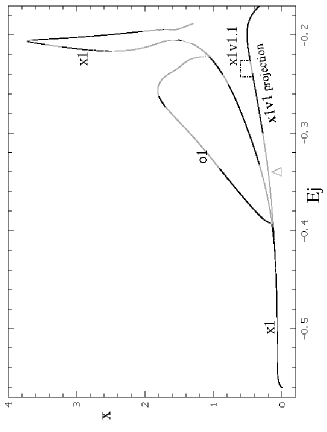
Figure 16: Characteristic diagram for some important families in model D. The unstable region of x1v1 bridged by x1v1.1 is indicated by a dashed-dotted line.

is a characteristic diagram of families x1, o1 and also of the ($E_{j}$,$x$) projection of the characteristic of the 3D family x1v1. The rising part of the branch of the x1 characteristic, for $E_{j}<-0.205$, is steeper than in model A1. In this model x1 is mainly stable at its decreasing branch ($E_{j}>-0.205$). The morphology of the x1 orbits there is rectangular-like, and this clearly shows that the model with a stronger bar favours this morphology.

The behaviour of x2 in model D is similar to that in model A1. The variation of the stability indices of x1 introduces as first bifurcating family in the system family x1v1. This has first a short stable part and then becomes complex unstable. The branch on Fig. 16 indicated by x1v1 is just the ($E_{j}$,$x$) projection of its characteristic curve. On this curve we note with $\Delta$ the complex unstable part. In the S$\rightarrow$$\Delta$ transition there is no family inheriting the stability of x1v1 when the latter becomes unstable. As a result, the only stable family for $-0.38<E_{j}<-0.338$ is the o1 family, which we also found in the slow bar case. If, at a given energy, we consider the two representatives of this family which are symmetric with respect to the major axis of the bar, we get the combined morphology shown in Fig. 17.

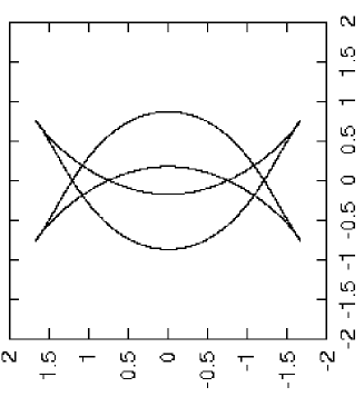
Figure 17: Two o1 orbits in model D, symmetric with respect to the major axis of the bar.

We should also note that the $(x,y)$ projection of the x1v1 family, away from the family’s bifurcating point, does not quite follow the morphological evolution of x1 at the same energy. The $(x,y)$ projections get squeezed on the sides already before they become rectangular shaped and thus tend to take a shape like ‘8’. This happens just before $|z|$ reaches values larger than 2 kpc. This morphology as well as the morphology of family x1v1.1, which bridges a small zone of simple instability of x1v1, can be seen in Fig. 18.

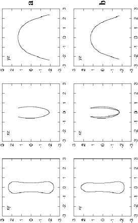
Figure 18: Orbits of the families x1v1 (a) and x1v1.1 (b) in model D at $E_{j}\approx-0.225$ and $-0.235$ respectively.

To summarise the specific features of the orbital structure of model D it is worth underlining that, due to its stronger bar, the x1v1 family bifurcates at lower energies than in the other models. After it bifurcates from x1 as stable it has, as usual, a complex unstable part, but beyond the $\Delta$$\rightarrow$S transition the orbits have still low $\overline{|z|}$. Another interesting feature is the stability of the x1 family at the decreasing part of the characteristic. Also, as in model B, families x1v5 and x1v5^′ exist and have stable representatives. Finally we note that from the families bifurcated initially as unstable, only x1v6 has away from the bifurcating point a small stability part.

6 Conclusions

In this paper we investigated the orbital structure in a class of models representing 3D galactic bars. The parameters we varied are the pattern speed, the strength of the bar and parameters defining the bulge component of the galactic model. We found all the families that could play an important role in the dynamics of 3D bars, and we registered the main changes which happen as we vary the parameters under consideration. Since evolutionary scenarios of the morphology of the bars within a Hubble time could include an increase of the bulge mass and a deceleration of the bar, as well as an increase or decrease of the bar’s strength, our models could correspond to discrete phases in the dynamical evolution of a barred galaxy. They could thus be used to explain the changes in the underling dynamics when the galaxies evolve. Similarly, they can be used to understand the dynamics of selected snapshots of $N$-body simulations.

Our main conclusions in the present paper are:

1. In all models we examined, the extent of the orbits which are most appropriate to sustain 3D bars is confined inside the radial 4:1 resonance. Viewing the models face-on, the orbits with the longest projections along the major axis of the bar are either boxy or elongated with loops at the major axis; these are typical shapes of the orbits in the radial 4:1 resonance region. This behaviour is common to both slow and fast rotating bars.

2. The evolution of the characteristic of the basic family x1 depends heavily on the pattern speed. The slower the bar rotates, the more complicated the x1-characteristic curve becomes. In the slowest of our models the families x1, x2 and x3 share the same characteristic curve. The folding of the characteristic towards lower energies, with most extreme case the one with the slow rotating bar, corresponds to a ‘bow’ feature in the evolution of the stability indices as function of $E_{j}$.

3. The fast rotating bar model A3 did not have the complicated evolution in the x1 characteristic and in the stability diagram corresponding to the ‘bow’. In this case all main 3D families of the x1-tree bifurcate from x1 at an S$\rightarrow$U transition before the local maximum of the x1-characteristic at the radial 4:1 resonance and have initial conditions $(x,z,0,0)$.

4. The bars can be supported not only by x1-originated families but, depending on the model, by 3D orbits bifurcated from families related with the z-axis orbits. This has been encountered in the case of a model without radial or vertical 2:1 resonances.

5. Slow pattern rotation favours the presence of 3D x2-type orbits along the minor axis of the main bar. These orbits, which can lead to a 3D inner bar, are typical orbits of the potentials we studied.

6. The most elongated 4:1 rectangular-like orbits have been encountered in the fast rotating bar model A3. On the contrary, the corresponding orbits in the slow bar of model A2 are square-like and farther out circles and orbits with circular-like $(x,y)$ projections. Thus in the slow bar case the bar is supported only by elliptical-like orbits of the x1-tree. The different elongations of the rectangular-like orbits can be explained by the fact that we have, in all models considered, bars of the same length in the imposed potential. Since the corotation radius changes with pattern speed, the non-axisymmetric part of the forcing is relatively larger near corotation for the fast bar than for the slow one.

7. The decreasing part of the x1-characteristic is in most cases unstable, except for the strong bar case (model D). This favours the presence of rectangular-like orbits at the outer parts of strong bars, in good agreement with observations (Athanassoula, Morin, Wozniak et al. 1990). This could be due to the fact that the bar forcing is stronger in the strong bar case. Stable rectangular-like orbits can also be found in the case of the fast rotating model A3, where rectangular-like stable orbits are provided not by the family x1 but by the families q0 and x1v8. This could again be due to the fact that, in the fast bar case, the forcing in the corotation region is larger than in other cases. The two above put together seem to argue that a strong bar forcing in the region around corotation is necessary for the model to have stable rectangular-like orbits which are sufficiently elongated along the bar major axis.

8. Models with low mass concentrations at the center (models B and C) favour the presence of $zn$ bifurcations for low $n$, which in some cases may be important for the global dynamics of the system (e.g. family z3.1s in model B). In this way we can have bar supporting families unrelated with the x1-tree.

9. In the x1-tree we encounter complex instability mainly in the x1v1 family. It can however, happen (e.g. in model C) that complex instability appears in large energies and thus all orbits with $\overline{|z|}<2$ kpc are stable. One must examine in every case the extent in $z$ of the complex unstable orbits of x1v1 in order to decide about the significance of this family for a model.

The connection between the families of periodic orbits and the observed morphologies in edge-on disc galaxies is discussed in paper III, and the contribution of orbital theory to the question of the boxiness of the outer isophotes in early type bars in paper IV.

Appendix A Poincaré’s ‘deuxième genre’ families in Hamiltonian systems

The number $n$ of intersections of a periodic orbit with the Poincaré surface of section, when the orbit has a particular direction, defines its multiplicity. So a periodic orbit of multiplicity $n$ has $n$ points of intersection with the Poincaré surface of section and it is called a periodic orbit of period $n$.

The linear stability or instability of a periodic orbit is defined by the eigenvalues of the corresponding monodromy matrix (see for example Yakubovich & Starzhinskii 1975). The columns of this matrix are suitably chosen linearly independent solutions of the so-called variational equations. These equations describe the time evolution of a small deviation from the periodic orbit. The eigenvalues of the monodromy matrix of a periodic orbit can be grouped as pairs of inverse numbers, i.e. if $\lambda$ is an eigenvalue then $1/\lambda$ is also an eigenvalue (Broucke 1969, Contopoulos & Magnenat 1985). The stability index $b$ that corresponds to a particular pair of eigenvalues is defined as:

$$b=-\left(\lambda+\frac{1}{\lambda}\right)$$ (1)

An orbit is stable when both stability indices are real numbers in the interval $(-2,\,2)$, which equivalently means that the corresponding eigenvalues are complex conjugate numbers on the unit circle.

As a parameter of the dynamical system changes the eigenvalues move on the complex plane. When two eigenvalues moving on the unit circle coincide on $\lambda=1$ and split along the real axis, the stability type of the orbit changes from stable to unstable. The corresponding stability index is negative and decreases below $-2$. At the same time a new periodic orbit of the same multiplicity is born. If, on the other hand, the two eigenvalues continue to lie on the unit circle, after coinciding on $\lambda=1$, which means that the orbit remains stable, then two new orbits of the same multiplicity are born. A periodic orbit of multiplicity $1$ can be also considered as a periodic orbit of multiplicity $n>1$ if it is repeated $n$ times. It has as monodromy matrix $M_{n}$ the matrix

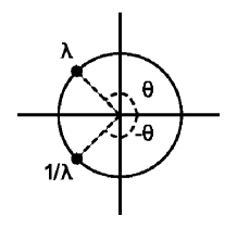
Figure 19: The eigenvalues of a stable orbit on the unit circle.

$$M_{n}=M^{n}_{1},$$ (2)

where $M_{1}$ is the monodromy matrix of the periodic orbit considered as 1-periodic. If the periodic orbit of period $1$ is stable, then it has a pair of eigenvalues of the form

$$\lambda=\cos\vartheta+i\sin\vartheta\,,\>\>\>\frac{1}{\lambda}=\cos\vartheta-i\sin\vartheta\,,$$ (3)

as seen in Fig. 19. Thus the corresponding stability index is:

$$b=-\left(\lambda+\frac{1}{\lambda}\right)=-2\cos\vartheta.$$ (4)

Considering this orbit as one of period $n$ its eigenvalues will be of the form $\lambda^{n}$, $(1/\lambda)^{n}$, so that the corresponding stability index $b_{(n)}$becomes:

$$b_{(n)}=-2\cos(n\vartheta).$$ (5)

A tangency of $b_{(n)}$ with the line $b=-2$ gives birth to two new periodic orbits of period $n$, while the 1-periodic orbit remains stable. This bifurcation happens when

$$b_{(n)}=-2\Rightarrow\cos(n\vartheta)=1$$ (6)

This condition is satisfied if we have e.g.

$$\vartheta=2\pi\frac{1}{n},$$ (7)

or equivalently when the stability index $b$ of the period $1$ periodic orbit crosses the line

$$b=-2\cos\left(2\pi\frac{1}{n}\right).$$ (8)

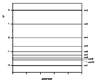
Figure 20: The values of the stability index $b$ that correspond to bifurcations of period $n=1,2,...,10$ given by Eq. (8).

The bifurcating families of periodic orbits are the ‘deuxième genre’ families of Poincaré (1899). In Fig. 20 we plot the lines given by (8) corresponding for $n=1,2,...10$. We see that, as we approach $b=-2$, the density of the lines as well as the period of the bifurcating orbit increase.

References

- [Athanassoula 1992a] Athanassoula E., 1992a, MNRAS 259, 328
- [Athanassoula 1990] Athanassoula E., Morin S., Wozniak H., Puy D., Pierce M. J., Lombard, J., Bosma, A., 1990, MNRAS 245, 130
- [Broucke 1969] Broucke R., 1969, NASA Techn. Rep. 32, 1360
- [Combes & Elmegreen 1993] Combes F., Elmegreen B.G., 1993, A&A 271,391
- [Contopoulos & Grosbøl 1989] Contopoulos G., Grosbøl P., 1989, A&AR 1,261
- [Contopoulos & Magnenat 1985] Contopoulos G., Magnenat P., 1985, Celest. Mech. 37, 387
- [Heisler et al. 1982] Heisler J., Merritt D., Schwarzschild M., 1982, ApJ 258, 490
- [Lindblad 1999] Lindblad P.O., 1999, A&ARv 9, 221
- [Lynden-Bell 1979] Lynden-Bell D., 1979, MNRAS 187, 101
- [Patsis et al. 2002a] Patsis P.A., Skokos Ch., Athanassoula E., 2002a (paper III - in preparation)
- [Patsis et al. 2002b] Patsis P.A., Skokos Ch., Athanassoula E., 2002b (paper IV - in preparation)
- [Papayannopoulos & Petrou 1983] Papayannopoulos T., Petrou M., 1983, A&A 119, 21
- [Pfenniger 1984] Pfenniger D., 1984, A&A 134, 373
- [Poincaré 1899] Poincaré H, 1899, ‘Les Methodes Nouvelles de la Mechanique Celeste’, Vol. III, Gauthier-Villars, Paris
- [Polyachenko & Polyachenko 1994] Polyachenko V.L., Polyachenko E.V., 1994, AstL 20, 416
- [Skokos et al. 2002] Skokos Ch., Patsis P.A., Athanassoula E., 2002 MNRAS, paper I this issue
- [Yakubovich & Starzhinskii] Yakubovich V. A., Starzhinskii V. M., 1975, ‘Linear Differential Equations with Periodic Coefficients’, Vol. 1, J. Wisley, New York
Acknowledgments
We acknowledge fruitful discussions and very useful comments by Prof. G. Contopoulos. We thank the referee for useful suggestions that allowed to improve the presentation of our work. This work has been supported by EET II and K 1994-1999; and by the Research Committee of the Academy of Athens. Ch. Skokos and P.A. Patsis thank the Laboratoire d’Astrophysique de Marseille, for an invitation during which essential parts of this work have been completed.