Orbital dynamics of three-dimensional bars:
I. The backbone of 3D bars. A fiducial case

Abstract

In this series of papers we investigate the orbital structure of 3D models representing barred galaxies. In the present introductory paper we use a fiducial case to describe all families of periodic orbits that may play a role in the morphology of three-dimensional bars. We show that, in a 3D bar, the backbone of the orbital structure is not just the x1 family, as in 2D models, but a tree of 2D and 3D families bifurcating from x1. Besides the main tree we have also found another group of families of lesser importance around the radial 3:1 resonance. The families of this group bifurcate from x1 and influence the dynamics of the system only locally. We also find that 3D orbits elongated along the bar minor axis can be formed by bifurcations of the planar x2 family. They can support 3D bar-like structures along the minor axis of the main bar. Banana-like orbits around the stable Lagrangian points build a forest of 2D and 3D families as well. The importance of the 3D x1-tree families at the outer parts of the bar depends critically on whether they are introduced in the system as bifurcations in $z$ or in $\dot{z}$.

1 Introduction

A thorough understanding of the orbital structure in a barred galaxy potential can provide useful insight to the stellar dynamics of barred galaxies and therefore to the dynamical evolution of these objects, as reviewed e.g. by Athanassoula (1984), Contopoulos & Grosbøl (1989), Sellwood & Wilkinson (1993) and Pfenniger (1996). Stable periodic orbits trap around them regular orbits and thus constitute the backbone of galaxy structure (Athanassoula, Bienayme, Martinet et al. 1983). Thus the appearance of a given morphological feature can often be associated with the properties of one of the main families of periodic orbits. In the ’90s, starting with Athanassoula (1992a; 1992b), many papers have pointed out that the gaseous response to steady barred potentials is, to a large degree, determined by the morphology of the periodic orbits in the corresponding stellar case. Thus, orbital and gaseous dynamics are linked. This has provided added incentive for studies of the morphology and the stability of periodic orbits in Hamiltonian systems representing disc galaxies.

Orbital theory has often provided useful information on the structure of galactic bars. Thus it is now understood that a bar is basically due to regular orbits trapped around the so called ‘x1’ periodic orbits, which are elongated along the bar major axis [Contopoulos & Grosbøl 1989]. Such orbits do not extend beyond the corotation resonance, and in many cases no suitable elongated orbits can be found beyond the 4:1 resonance. This led orbital theory to predict that bars should end at or before corotation [Contopoulos 1980]. Orbital theory was also able to predict - at the right distance from the center - the loops of the near-infrared isophotes (see the case of NGC 4314 in Patsis, Athanassoula & Quillen 1997). Yet not all important morphological features have been so far explained with the help of periodic orbits. Thus orbital theory has difficulties to explain the boxy isophotes surrounding the bars of, mainly, early-type barred galaxies (Athanassoula 1996, Patsis et al. 1997). Another point still under discussion is the morphology of the peanut-shaped bulges observed in edge-on disc galaxies. They are considered by many authors as revealing the presence of a bar, and to be associated with the 2:1 vertical resonance. It is not clear, however, which families can make this vertical structure. Could a bar without a vertical 2:1 resonance be boxy or peanut-shaped when viewed edge-on? Could we have stellar rings out of the equatorial plane at the ILR region? Furthermore, the detailed dynamics of the corotation region and the differences in the vertical structure between fast and slow bars remain open issues.

In this series of papers we use orbital theory to address the above questions. This is a first step towards understanding both the orbital behavior in $N$-body models and the responses of gaseous discs to potentials derived from near-infrared observations. The differences between our model and the well studied corresponding 2D case of the Ferrers bar [Athanassoula 1992a] reflect the changes due to the inclusion of the third dimension. In separate papers we address the question of the morphology of the peanut shaped-bulges (Patsis, Skokos & Athanassoula, 2002a - paper III) and of the boxy isophotes of bars seen face-on (Patsis, Skokos & Athanassoula, 2002b - paper IV).

Our first goal is to make a thorough study of the orbital structure in 3D barred potentials, to classify the important families, and to follow their morphological evolution as a function of the Jacobi integral. We start with a fiducial case. Many of the families we find in this model have been previously mentioned (e.g Heisler, Merritt & Schwarzschild 1982; Pfenniger 1984, 1985b; Martinet & de Zeeuw 1988; Hasan, Pfenniger & Norman 1993). However, other, equally important families, have not yet been studied.

Studying the orbital stability in a Hamiltonian system approximating the dynamics of a barred galaxy we get the periodic orbits that could be used as building blocks for a density model. The general rule is to look for stable periodic orbits, since they trap around them the regular orbits. Not all of them, however, are equally important. The isodensities of the model we use show us the topological limits within which we should look for the significant orbits. Stable representatives of families of periodic orbits which do not support the imposed morphology, i.e. that of a bar embedded in an axisymmetric disc with a central bulge, should be considered as less important. As an example, in 2D models, let us mention the case of the retrograde family x4, which is stable over a very large interval of energies (Athanassoula et al. 1983). This family, however, should get a minimum weight when one tries to construct a self consistent model using a Schwarzschild (1979) or a Contopoulos & Grosbøl (1988) method. In a model of a 3D disc galaxy, besides the counter-rotating x4 family on the equatorial plane, one has to filter out also stable orbits with large $\overline{|z|}$, i.e. orbits with large mean vertical deviations, since these orbits do not contribute much to the density of the barred galaxy.

This paper is organized as follows: In section 2 we review briefly the parts of orbital theory that are necessary for understanding this paper. In particular we explain the use of characteristic and stability diagrams in following the dynamical evolution of a family of periodic orbits. We describe also the various types of instabilities encountered in 3D Hamiltonian systems and we introduce the nomenclature of the main families. The latter is necessary since a number of the families presented here have not been previously discussed and thus need to be incorporated in a unique nomenclature scheme. In section 3 we introduce our 3D model and the orbital structure in a 2D counterpart. In section 4 we present the main families x1, x2 and x3 and their bifurcations. In section 5 we describe the orbits around L₄ (or L₅) and around L₁ (or L₂), as well as families outside corotation. We conclude in section 6.

2 A short introduction to periodic orbits in the present context

2.1 Periodic orbits and their stability

In this section we will briefly review some parts of orbital theory which are necessary for the understanding of this paper. A clear, easily readable introduction to the subject has been given by Sellwood & Wilkinson (1993). We also refer the reader to the pioneering works of Pfenniger (1984, 1985b) and Contopoulos & Magnenat (1985).

We study the stability of simple-periodic orbits in a barred potential in cartesian coordinates. The 3D bar is rotating around its short $z$ axis. The $x$ axis is the intermediate and the $y$ axis the long one. The system is rotating with an angular speed $\Omega_{b}$ and the Hamiltonian governing the motion of a test-particle can be written in the form:

$$H=\frac{1}{2}(p_{x}^{2}+p_{y}^{2}+p_{z}^{2})+V(x,y,z)-\Omega_{b}(xp_{y}-yp_{x}),$$ (1)

where $p_{x},~{}p_{y},$ and $p_{z}$ are the canonically conjugate momenta. We will hereafter denote the numerical value of the Hamiltonian by $E_{j}$ and refer to it as the Jacobi constant or, more loosely, as the ‘energy’. The corresponding equations of motion are:

$$\dot{x}=p_{x}+\Omega_{b}y, \dot{y}=p_{y}-\Omega_{b}x, \dot{z}=p_{z}$$

$$\dot{p_{x}}=-\frac{\partial V}{\partial x}+\Omega_{b}p_{y}, \displaystyle{\dot{p_{y}}=-\frac{\partial V}{\partial y}-\Omega_{b}p_{x},} \dot{p_{z}}=-\frac{\partial V}{\partial z}$$ (2)

The space of section in the case of a 3D system is 4D. The equations of motion are solved for a given value of the Hamiltonian, starting with initial conditions $(x_{0},\dot{x}_{0},z_{0},\dot{z}_{0})$ in the plane $y$=0, for $\dot{y}>0$. The next intersection with the $y$=0 plane with $\dot{y}>0$ is found and the exact initial conditions for the periodic orbit are calculated using a Newton iterative method. A periodic orbit is found when the initial and final coordinates coincide with an accuracy at least 10^-10. The integration scheme used was a fourth order Runge-Kutta scheme.

The estimation of the linear stability of a periodic orbit is based on the theory of variational equations. We first consider small deviations from its initial conditions, and then integrate the orbit again to the next upward intersection. In this way a transformation $T:\mathbf{R}^{4}\to\mathbf{R}^{4}$ is established, which relates the initial with the final point. The relation of the final deviations of this neighboring orbit from the periodic one, with the initially introduced deviations can be written in vector form as: $\vec{\xi}=M\,\vec{\xi_{0}}$. Here $\vec{\xi}$ is the final deviation, $\vec{\xi_{0}}$ is the initial deviation and $M$ is a $4\times 4$ matrix, called the monodromy matrix. It can be shown that the characteristic equation is written in the form $\lambda^{4}+\alpha\lambda^{3}+\beta\lambda^{2}+\alpha\lambda+1=0$. Its solutions $(\lambda_{i},i=1,2,3,4)$ obey the relations $\lambda_{1}\,\lambda_{2}=1$ and $\lambda_{3}\,\lambda_{4}=1$ and for each pair we can write:

$$\lambda_{i},1/\lambda_{i}=\frac{1}{2}[-b_{i}\pm(b_{i}^{2}-4)^{\frac{1}{2}}],$$ (3)

where $\displaystyle b_{i}=1/2\,(\alpha\pm\Delta^{1/2})$ and $\Delta=\alpha^{2}-4(\beta-2)$.

The quantities $b_{1}$ and $b_{2}$ are called the stability indices. If $\Delta>0$, $|b_{1}|<2$ and $|b_{2}|<2$, the 4 eigenvalues are on the unit circle and the periodic orbit is called ‘stable’. If $\Delta>0$, and $|b_{1}|>2$, $|b_{2}|<2$, or $|b_{2}|>2$, $|b_{1}|<2$, two eigenvalues are on the real axis and two on the unit circle, and the periodic orbit is called ‘simple unstable’. If $\Delta>0$, $|b_{1}|>2$, and $|b_{2}|>2$, all four eigenvalues are on the real axis, and the periodic orbit is called ‘double unstable’. Finally, $\Delta<0$ means that all four eigenvalues are complex numbers but off the unit circle. The orbit is characterized then as ‘complex unstable’ (Contopoulos & Magnenat 1985, Heggie 1985, Pfenniger 1985a,b). We use the symbols $S,\>U,\>D,\>\Delta$ to refer to $stable$, $simple~{}unstable$, $double~{}unstable$ and $complex~{}unstable$ periodic orbits respectively. For a general discussion of the kinds of instability encountered in Hamiltonian systems of N degrees of freedom the reader may refer to Skokos (2001).

The method described above has been initially presented by Broucke (1969) and Hadjidemetriou (1975), and has been used in studies of the stability of periodic orbits in systems of three degrees of freedom. The reader is referred to Pfenniger (1984) and Contopoulos & Magnenat (1985) for an extended description.

A diagram that describes the stability of a family of periodic orbits in a given potential when one of the parameters of the system varies (e.g. the numerical value of the Hamiltonian $E_{j}$), while all other parameters remain constant, is called a ‘stability diagram’ (Contopoulos & Barbanis 1985, Contopoulos & Magnenat 1985). With the help of such a diagram one is able to follow the evolution of the stability indices $b_{1}$ and $b_{2}$, and the transitions from stability to instability or from one to another kind of instability. We will loosely refer to the $b=2$ and $b=-2$ lines on a stability diagram as the $b=2$ and $b=-2$ axes. The S$\rightarrow$U transitions, when one of the stability indices has an intersection with the $b=-2$ axis, or tangencies of the stability curves with the $b=-2$ axis, are of special importance for the dynamics of a system. In this case a new stable family is generated by bifurcation of the initial one and has the same multiplicity as the parent family. That means that the periodic orbits of the bifurcating family have, before closing, as many intersections with the plane $y$=0, for $\dot{y}>0$, as the orbits of the parent family. The new family may play an important role in the dynamics of the system. S $\rightarrow$U transitions after an intersection of a stability curve with the $b=2$ axis, or tangencies of a stability curve with the $b=2$ axis, also generate a stable family but are accompanied by period doubling. This means that the number of intersections with the plane $y$=0 (always with $\dot{y}>0$), needed for the periodic orbits to close, is double the corresponding number of the parent family. Since the most important families we examine here are simple-periodic, i.e. of multiplicity 1, intersections or tangencies of their stability indices with the $b=2$ axis introduce in the system families of orbits with multiplicity 2. U$\rightarrow$D and D$\rightarrow$$\Delta$ transitions do not bring new stable families in the system and thus in principle are only of theoretical interest. As we will see, however, the evolution of a family which is found to be initially unstable may be very important for the dynamics of our model. The family could simply become stable in another energy interval, or it may play a major role in a collision of bifurcations, an inverse bifurcation or other dynamical phenomena [Contopoulos 1986]. Finally in the case S$\rightarrow$$\Delta$ we have in general no bifurcating families of periodic orbits.

Another very useful diagram is the ‘characteristic’ diagram [Contopoulos & Mertzanides 1977]. It gives the $x$ coordinate of the initial conditions of the periodic orbits of a family as a function of their Jacobi constant $E_{j}$. In the case of orbits lying on the equatorial plane and starting perpendicular to the $x$ axis, we need only one initial condition, $x$, in order to specify a periodic orbit on the characteristic diagram. Thus, for such orbits this diagram gives the complete information about the interrelations of the initial conditions in a tree of families of periodic orbits and their bifurcations. However, even for orbits completely on the equatorial plane, but not starting perpendicular to the $x$ axis we need to give initial conditions as position–velocity pairs $(x,\dot{x})$ and the characteristic diagram is three-dimensional $(E_{j},x,\dot{x})$. In the general case of orbits in a 3D system, one has a set of four initial conditions and the characteristic diagram is five-dimensional. The representation of such a diagram is difficult, but when necessary we will give just the $(E_{j},x)$ projection. $(E_{j},x)$ diagrams that can be compared with the corresponding 2D models will always be given. In all characteristic diagrams the region to which the orbits are confined is bounded by a curve known as the zero velocity curve (ZVC), since the velocity on it becomes zero.

2.2 The nomenclature of the main families

Our orbital study is more extended than previous ones and thus brings in new families of orbits which have not been studied so far. We were thus brought to introduce a new nomenclature system, extension of the Contopoulos & Grosbøl (1989) system, which covers all the new types of orbits.

For the main 2D families of simple periodic orbits the nomenclature in the present paper follows the standard notation of Contopoulos & Grosbøl (1989). We thus have the x1 family, where orbits are elongated along the bar and which is the main family in the case of barred potentials, families x2 and x3, whose orbits are elongated perpendicular to the bar, and the retrograde family x4. 2D families bifurcated from x1 at the 3:1 resonance region on the equatorial plane are denoted by t1, t2, …, for consistency with the names used in Patsis et al. (1997). 2D families bifurcated at the 4:1 resonance region on the equatorial plane are called q1, q2, q3,…. Planar orbits related with the 1:1 radial resonance will be called o1, o2…. They are encountered only in some models. The fiducial case presented in the present paper is not one of them.

Further planar families appear beyond the x1 family, at the gaps of the even resonances 4:1, 6:1, 8:1 etc. They are given the names ‘f’, ‘s’, ‘e’… respectively. These families, not directly related to the morphological problems we address in this series, will be discussed elsewhere.

We name the 3D families bifurcated from the basic family x1 at the vertical resonances as x1v$n$, where $n$ denotes the order of their appearance in our fiducial model A (see below section 4). This is a convenient model to be used for our nomenclature, since there are families of 3D orbits associated with all basic vertical resonances. So x1v1 is the one bifurcated at the first S$\rightarrow$U transition, which happens at the vertical 2:1 resonance region, x1v2 is the one bifurcated at the U$\rightarrow$S transition (second stability transition of the model also at the vertical 2:1 resonance region), x1v3 is the one bifurcated at the S$\rightarrow$U transition at the vertical 3:1 resonance and so on. Further bifurcations of these x1v$n$ families are indicated with an ‘.$n$’ (for the $n$-th bifurcation) attached to the name of the parent family; i.e. the first bifurcation of x1v1 will be x1v1.1, the second x1v1.2, etc. Further bifurcations of these families will be indicated by further ‘.$n$’ attached to the name of the parent family. Thus x1v1.1.1 is the first bifurcation of x1v1.1. The naming system is thus extendable at will.

In general at each vertical resonance we have two bifurcating families introduced in the system. The number of oscillations along the rotation axis $z$ corresponds to the vertical resonance at which the family is born. E.g. families x1v1 and x1v2, which are bifurcated at the vertical 2:1 resonance region, have orbits with two oscillations along the $z$ axis. This determines only partially their morphology, since the bifurcating family can be introduced either in the $z$ or the $\dot{z}$ coordinate of the initial conditions. If we know the number of oscillations of a family along each axis and also whether it is a bifurcation in $z$ or $\dot{z}$, then we know its morphology. Families with similar morphology are similar in their corresponding $(x,y)$, $(x,z)$ and $(y,z)$ projections. In the fiducial case, where each vertical resonance is associated with two bifurcating families, the families x1v(2n-3) and x1v(2n-2) are born at the n:1 resonance.

We note, however, that the first vertical bifurcation is not in every model the x1v1 family, as in the fiducial case. In other models (Skokos, Patsis & Athanassoula, 2002 - paper II) it can happen that the first 3D bifurcation of x1 is not related with the 2:1 vertical resonance, but with a different one. In such a model the first vertical bifurcation of x1 will have the same name as the family of the fiducial model which has similar morphology. Equivalently, it will have the same name as the family of the fiducial model which is introduced in the same n:1 resonance and in the same ($z$ or $\dot{z}$) coordinate. This way we make sure that families with similar morphologies share the same name in the various models. In addition, if for some reason we have more than one vertical bifurcation of x1 associated with a vertical resonance, we introduce appropriate primes in our nomenclature. E.g. in a model with two vertical 4:1 resonances we will have the pairs of bifurcating families x1v5, x1v6 and x1v5^′, x1v6^′. By keeping the basic name of the family similar for all families associated with the same vertical resonance, we underline again the dependence of the name on the encountered morphology. Nevertheless, the basic names are given in the fiducial model, which thus becomes a reference case for all our work.

We use the same nomenclature not only for the bifurcations of the basic family x1, but in general for the vertical bifurcations of every 2D family. Their name consists of the name of the parent family, followed by ‘v$n$’, where $n$ indicates its $n$-th vertical bifurcation. Also the names of the bifurcations of the bifurcating families are characterized by the addition of ‘.1’, ‘.2’$\dots$ etc. at the end of the name of the 3D family, as described above for the corresponding families associated with x1.

We will use the same system in order to name also radially bifurcating families. In general a radial bifurcation will be named as ‘wr$n$’, where ‘w’ the name of the parent family. E.g. the $n$-th radial bifurcation of family f will be ‘fr$n$’ (fr1, fr2…etc.).

Let us now turn to orbits related with the axis of rotation. The family on the axis of rotation is called ‘z-axis’ family [Martinet & de Zeeuw 1988]. Its two first bifurcations are introduced at the first S$\rightarrow$U transition and the first U$\rightarrow$S transition respectively and they are the ‘sao’ and ‘uao’ orbits of Heisler, Merritt & Schwarzschild (1982). This nomenclature, however, does not lend itself to extension which can include what Poincaré (1899) called the ‘deuxième genre’ families (cf. Polymilis, Servizi & Skokos, 1997) which can play an important role in some Ferrers bars (paper II), so we will not adopt it here for other families related with the z-axis orbits. In practice ‘deuxième genre’ orbits are found on the stability diagrams as bifurcations of the parent family when this family is considered as being of higher multiplicity, i.e. if its orbits are repeated many times. Thus, the z-axis family, when its orbits are repeated twice, is called z2. Bifurcations of the z2 family are called z2.1, z2.2 etc. The same rule applies for the bifurcations of z3, i.e. for the bifurcations of z-axis if this is described three times. We then have z3.1, z3.2 and so on. These bifurcating families always come in pairs. A further index (s or u) is attached to their names and is related with their stability.

Around the Lagrangian points $L_{4,5}$ we have the long period banana-like orbits, which form a tree of families, and the short period orbits. For the latter we keep the Contopoulos & Grosbøl (1989) notation (spo). For the banana-like orbits we use the notation ban1, ban2,…ban$n$ in the 2D cases. Their 2D bifurcations are the families ban$n$.1, ban$n$.2,… etc. and their 3D bifurcations the families ban$n$v1, ban$n$v2,… etc. 3D banana-like orbits not related with a 2D one are named banv$n$.

A 2D family found around the unstable Lagrangian points $L_{2,3}$ is called $\ell_{1}$.

Throughout the papers we give also the names used by other authors for families that have been previously studied. However, since our study is more extended, there are several families mentioned for the first time.

3 The model

3.1 The 3D potential

For our calculations we used a 3D potential, which consists of a Miyamoto disc, a Plummer bulge and a Ferrers bar. Pfenniger and collaborators have made extensive use of this potential for orbital calculations (Pfenniger 1984, Pfenniger 1985a;b, Martinet & Pfenniger 1987, Pfenniger 1987, Pfenniger 1990, Hasan, et al. 1993, Olle & Pfenniger 1998). Our work is, in many ways, more extended. We make a much more extensive search for periodic families and we furthermore follow their stability. The latter allows us to find a number of ‘new’ families, which show interesting morphological characteristics. Furthermore, we vary the parameters of the model so that we are able to make comparisons between fast and slow rotating bars as well as between strong and weak bars (paper II). Finally, we focus our work more on tracing the orbital behaviour that could support observed morphological features and less on studying in depth qualitatively the dynamical phenomena that take place in this kind of Hamiltonian systems.

Our general model consists of 3 components. The disc is represented by a Miyamoto disc (Miyamoto & Nagai 1975), the potential of which reads:

$$\Phi_{D}=-\frac{GM_{D}}{\sqrt{x^{2}+y^{2}+(A+\sqrt{B^{2}+z^{2}})^{2}}},$$ (4)

where $M_{D}$ is the total mass of the disc, $A$ and $B$ are the horizontal and vertical scale lengths, and $G$ is the gravitational constant. The bulge is modeled by a Plummer sphere with potential:

$$\Phi_{S}=-\frac{GM_{S}}{\sqrt{x^{2}+y^{2}+z^{2}+\epsilon_{s}^{2}}},$$ (5)

where $\epsilon_{s}$ is the scale length of the bulge and $M_{S}$ is its total mass. The third component of the potential is a triaxial Ferrers bar, whose density $\rho(x)$ is:

$$\rho(x)=\left\{\begin{array}[]{lcc}\displaystyle{\frac{105M_{B}}{32\pi abc}(1-m^{2})^{2}}&{\mbox{f}or}&m\lid 1\\ &&\\ \displaystyle{0}&{\mbox{f}or}&m>1\end{array}\right.,$$ (6)

where

$$m^{2}=\frac{y^{2}}{a^{2}}+\frac{x^{2}}{b^{2}}+\frac{z^{2}}{c^{2}}\,\,,\,\,\,a>b>c,$$ (7)

$a$, $b$, $c$ are the semi-axes and $M_{B}$ is the mass of the bar component. The corresponding potential $\Phi_{B}$ and the forces are given in Pfenniger (1984). They are in a closed form, well suited for numerical treatment. For the Miyamoto disc we use A=3 and B=1, and for the axes of the Ferrers bar we set $a:b:c=6:1.5:0.6$, as in Pfenniger (1984). We note that these axial ratios are near the standard values given by Kormendy (1982). The masses of the three components satisfy $G(M_{D}+M_{S}+M_{B})=1$. The length unit is taken as 1 kpc, the time unit as 1 Myr and the mass unit as $2\times 10^{11}M_{\odot}$.

In Table 1 we give the parameters of our model. We give it the name A1, and it will be one of the models to be used in our comparative study in paper II.

Table 1: The parameters of our fiducial model A1. G is the gravitational constant, M_D, M_B, M_S are the masses of the disk, the bar and the bulge respectively, $\epsilon_{s}$ is the scale length of the bulge, $\Omega$_b is the pattern speed of the bar, $E_{j}$(r-IILR) and $E_{j}$(v-ILR) are the values of the Jacobi constant for the radial and vertical 2:1 resonances and $R_{c}$ is the corotation radius.

GMD	GMB	GMS	$\epsilon_{s}$	$\Omega$b	$E_{j}$(r-IILR)	$E_{j}$(v-ILR)	$R_{c}$
0.82	0.1	0.08	0.4	0.054	-0.44	-0.36	6.13

3.2 The 2D Ferrers bar

The general orbital structure in potentials including a 2D Ferrers bar can be found in Athanassoula (1992a). The dynamics are dominated by the presence of the x1 family, which is in general stable. It is characterized by the presence of a narrow instability zone at the 3:1 resonance and a gap at the 4:1 region, which is generally of type 2 [Contopoulos & Grosbøl 1989]. The S$\rightarrow$U$\rightarrow$S transition at the 3:1 region introduces in the system a couple of simple periodic families of orbits, the importance of which remains local. Beyond the type 2 gap and above the local maximum of the characteristic of x1 at the 4:1 resonance (Fig. 2 in Contopoulos & Grosbøl 1989) one can find a large number of families squeezed close to the zero velocity curve. Finally the families x2 and x3 generally exist for a large energy range and their characteristics form a single bubble. As it is known, x2 is generally stable and x3 unstable.

In the next sections we describe the orbital behaviour in a 3D case where both radial and vertical 2:1 resonances exist. We will thus find the differences introduced in the morphology and stability of the families of periodic orbits by the inclusion of the third dimension. We will also examine how the 3D families of periodic orbits support the bar.

4 The x1-family and its bifurcations

4.1 A general description

Contrary to the 2D models, where a single family, the x1 family, provides the building blocks for the bar, in 3D models we have a tree of families consisting of 2D and 3D families related to the planar x1 orbits. In Table 2 we summarize the properties of these families. We list their name, the value of the energy at which they are born ($E_{j}^{*}$), the $E_{j}$ intervals where they are stable and we indicate whether they are two-dimensional (2D) or three-dimensional (3D). Their interconnections and their role will be described in the following paragraphs.

Table 2: The families of the x1-tree. The successive columns give the name of the families, the value of the energy at which they are introduced ($E_{j}^{*}$), the intervals of $E_{j}$ at which they are stable and also if they are 2D or 3D. The ‘bow’-region is explained in the text, while ‘…’ after an energy value indicate that a family continues to be stable, but reaches distances far away from the $z=0$ plane.

family	$E_{j}^{*}$	stable intervals in $E_{j}$	2D / 3D
x1	$-0.495$	$-0.495<E_{j}<-0.360$	2D
		$-0.343<E_{j}<-0.293$
		$-0.278<E_{j}<-0.244$
		‘bow’-region $-0.222<E_{j}<-0.214$
		$-0.211<E_{j}<-0.205$
		$-0.192<E_{j}<-0.191$
		$-0.186<E_{j}<-0.185$
		$-0.175<E_{j}<-0.173$
x1v1	$-0.360$	$-0.360<E_{j}<-0.336$	3D
		$-0.253<E_{j}<-0.147\,\ldots$
x1v2	$-0.343$	always unstable	3D
x1v3	$-0.293$	$-0.293<E_{j}<-0.221$	3D
x1v4	$-0.278$	$-0.224<E_{j}<-0.149$	3D
x1v5	$-0.213$	$-0.213<E_{j}<-0.172$	3D
x1v6	$-0.211$	always unstable	3D
x1v7	$-0.205$	$-0.205<E_{j}<-0.183$	3D
		$-0.174<E_{j}<-0.170$
x1v8	$-0.192$	always unstable	3D
x1v9	$-0.185$	$-0.185<E_{j}<-0.182$	3D

There are also several 2D families, which are radial bifurcations of x1 and thus part of the x1-tree, but play a less important role in the morphology of the models. They are described in a separate table (Table 3). The ‘t’ families are related with the 3:1 and the ‘q’ with the 4:1 radial resonance region.

Table 3: Radial bifurcations of the x1 family. ‘t’ families are related with the 3:1 and ‘q’ families with the 4:1 radial resonance region. Columns are as in Table 2. $E_{j}$ values are given in general with three digits, except from the cases where narrow $E_{j}$ ranges of existence need more accuracy. We note that the t3 family exists also for lower energies than its $E_{j}^{*}$ (see section 4.4).

family	$E_{j}^{*}$	stable intervals in $E_{j}$	2D / 3D
t1	$-0.244$	$-0.244<E_{j}<-0.218$	2D
t2	$-0.214$	$-0.214<E_{j}<-0.209$,	2D
		$-0.204<E_{j}<-0.203$
t3	$-0.205$	$-0.2065<E_{j}<-0.2005$	2D
q1	$-0.191$	always unstable	2D
q2	$-0.1857$	$-0.1860<E_{j}<-0.1857$	2D
q3	$-0.183$	$-0.1818<E_{j}<-0.1808$	2D

Besides the orbits related to the x1 family, we find the x2 and x3 families and their 3D relatives as well. They exist for the same energy intervals as the families of the x1-tree, but their projections on the equatorial plane are elongated along the minor axis of the bar. They are described below.

4.2 Families x1, x2 and x3

The characteristics of the x1 and the x2-x3 families in model A1 (Fig. 1) have the typical geometry of the characteristics of 2D Ferrers bars [Athanassoula 1992a]. Due to the vertical instabilities, however, x1 becomes unstable over several $E_{j}$ intervals, and not only at the radial 3:1 resonance region, as in the 2D case. In Fig. 1 and in all characteristic diagrams hereafter we draw the unstable regions in light-grey. We observe that the decreasing part of the x1 curve, below the local maximum at the radial 4:1 resonance region ($E_{j}\approx-0.21$), is almost everywhere light-grey, indicating that the family is unstable there. The curve at about $E_{j}\approx-0.17$ turns back towards lower energies, remaining after that continuously unstable.

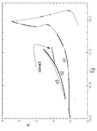
Figure 1: x1, x2-x3 and the x2mul2 $(E_{j},x)$-characteristics. The curve corresponding to x2mul2 is the projection of its characteristic on the $(E_{j},x)$ plane. Stable regions are drawn in black and unstable ones in light gray.

The morphological evolution of the x1 orbits is the one expected from the 2D case and is given in Fig. 2. The numbers at the upper right corners of the individual frames correspond to the $E_{j}$ value of the orbit. The orbits are chosen along the characteristic curve starting from the lower values of the Jacobi constant; the orbits in Fig. 2h,i,j belong to the decreasing branch. Except for the instability zones related to the 3:1 resonance all other unstable parts of x1 appear only in the 3D case. As mentioned in section 2.1, the families introduced at the instability strips by bifurcation inherit the kind of stability of the parent family, i.e. of x1. Thus, the instability gaps on the x1 characteristic are covered by the stable orbits of the families born after the corresponding S$\rightarrow$U transitions. So for almost every energy $E_{j}$ there exists a stable orbit of the x1-tree. As we mentioned in section 2, the 3D bifurcated families are in general characterized by four initial conditions $(x_{0},\dot{x}_{0},z_{0},\dot{z}_{0})$ so that a $(E_{j},x_{0})$ characteristic diagram cannot provide all the essential information. For this reason we prefer to follow the dynamical evolution of the orbits using stability diagrams.

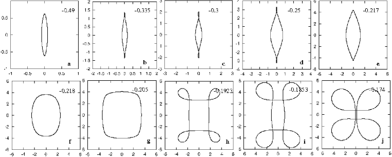
Figure 2: x1 stable orbits in model A1. The numbers at the upper right corners of the panels indicate their $E_{j}$ values.

These diagrams frequently become complicated, but they have the big advantage of giving in a straightforward way the interconnections of the various families, thus becoming a very useful tool in the hunting of periodic orbits.

The evolution of the stability indices $b_{1}$ and $b_{2}$ for x1 are given in Figs. 3,  4, and  5 for successive energy intervals. The arrows denote bifurcated families at the bifurcating points and show the direction of the stability index associated with the S$\rightarrow$U or U$\rightarrow$S transition. We observe that the variation of the

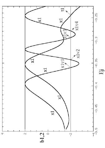
Figure 3: First part of the x1 stability diagram. Arrows denote the bifurcation of families and the direction in which these evolve.

index which in Fig. 3 has the larger values for $E_{j}<-0.38$ brings in the system the 3D families x1v1, x1v2 etc., while the variation of the other index brings in the families associated with the radial instabilities. The latter remain on the equatorial plane. The variation of their stability indices will in turn bring new families due to vertical and radial instabilities.

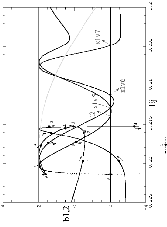
Figure 4: Second part of the x1 stability diagram. The evolution of the stability curves in the x1 ‘bow’ is indicated with numbers from 1 to 8 and arrows. In the diagram we indicate also the x1 bifurcations to the right of the ‘bow’. They are the families t2, x1v5, x1v6 and x1v7.

The feature depicted in Fig. 4 is typical of the stability diagrams of many of our models. We call this kind of evolution of the stability indices a ‘bow’. The $b_{1}$ and $b_{2}$ curves do not break anywhere, but they evolve in a continuous, rather complicated way, changing direction twice. This ‘bow’ area corresponds to the bend, or elbow, in the characteristic at about $E_{j}\approx-0.227$ (Fig. 1), and the complicated evolution of the stability indices happens as we move towards lower $E_{j}$ values along the characteristic curve of x1 at this area. In Fig. 4 one can follow the evolution of $b_{1}$ and $b_{2}$ by following the evolution of both the numbers and the nearby arrows. The lowest value of the stability index at ‘5’, not included in the Figure (indicated only with a dashed arrow outside of figure frame), is $\approx-55$.

A significant change in the way the 3D bifurcations of x1 are introduced in the system happens at the instability zone found just beyond the local maximum of the $(E_{j},x)$ characteristic close to the radial 4:1 resonance. As we see in Fig. 3, 4 and 5, the 3D families are bifurcated at S$\rightarrow$U and U $\rightarrow$S transitions, where the corresponding stability index intersects the $b=-2$ axis. Moving on the characteristic towards corotation, before reaching the decreasing branch, a bifurcating family at an S$\rightarrow$U transition is a stable 3D family with initial conditions $(x,z,\dot{x},\dot{z})=(a,b,0,0)$, where $a,b\in\mathbf{R}$ and $a,b\neq 0$. On the other hand, the family bifurcated at the U$\rightarrow$S transition, is (initially) simple unstable and has initial conditions $(x,z,\dot{x},\dot{z})=(c,0,0,d)$, with $c,d\in\mathbf{R}$ and $c,d\neq 0$. This means that the family introduced in the system as stable is a bifurcation at $z$, and the simple unstable family a bifurcation at $\dot{z}$. For the set of families associated with the vertical 5:1 resonance, on the decreasing branch of the characteristic, this sense of bifurcation is reversed. Namely we have the bifurcation in $z$ at the U$\rightarrow$S transition (x1v8) and the bifurcation in $\dot{z}$ at S$\rightarrow$U (x1v7).

In Fig. 5 we plot the last part of the stability diagram of the x1 family, corresponding to energies higher than $-0.2$.

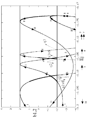
Figure 5: Stability diagram for x1 and bifurcating families corresponding to the decreasing part of the x1 characteristic. The evolution of the stability curves is indicated with numbers from 1 to 11, and thick arrows that point to the direction of the evolution. The bifurcating families and their direction of evolution are denoted with thin arrows.

As can be seen from the characteristic diagram of Fig. 1, this includes most of the decreasing part of the characteristic, the bend at $E_{j}\approx-0.173$ and the part that goes towards lower energies. This part (roughly for $-0.22<E_{j}<-0.173$), has negative $x$ values starting soon after the bend. Heavy arrows and numbers in increasing order on and next to the stability curves in Fig. 5 indicate the evolution of the indices as we move along this part of the characteristic. As we can see most parts are unstable, the short stable parts being drawn with heavy lines. After the turning point, at $E_{j}\approx-0.173$, the upper curve, moving now towards lower $E_{j}$ values, is stable until $E_{j}\approx-0.181$, then has a part with values smaller than $-2$ and then reenters the stability region for $E_{j}\approx-0.197$. The lower stability curve, however, reaches absolutely large negative values. Thus, the family is always unstable in the parts where $x<0$. It is easy to understand how the negative $x$ values are introduced by following the evolution of the x1 orbit morphology as we move along the characteristic (Fig. 2). As one moves along the decreasing part of the characteristic (Fig. 2h $\rightarrow$j), the four apocentra of the orbits develop loops, whose size increases strongly as the energy increases. Already for the orbit in Fig. 2j the loops have become so large, that the sides of the orbit along the bar major axis nearly touch. As we continue along the characteristic they will touch and then cross, so that $x$ becomes negative.

Let us now present the evolution of the x2-x3 loop in the 3D case. As seen in Fig. 1, the situation with the x2-x3 characteristic is exactly like in 2D. The stability indices form also loops, as the $b_{1}$ and $b_{2}$ indices of x2 and x3 join each other in pairs (Fig. 6).

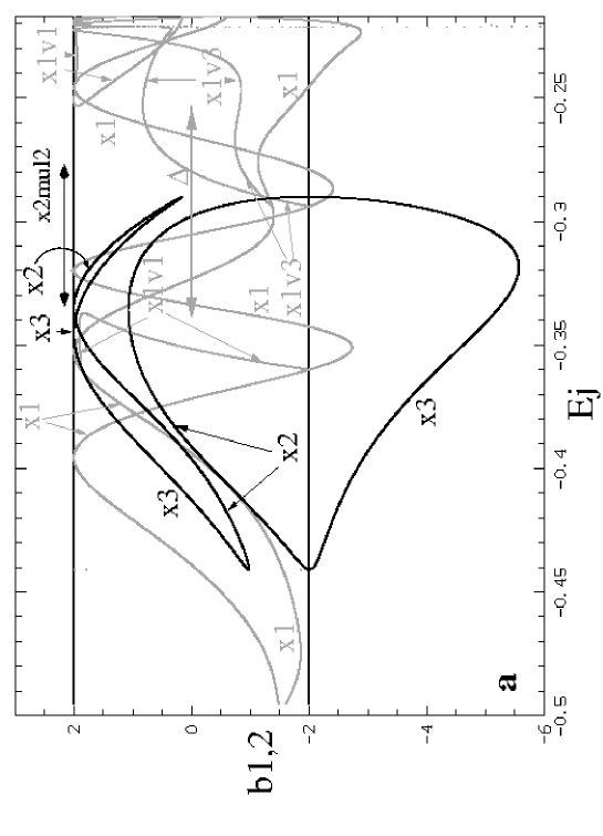
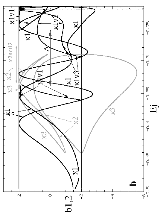
Figure 6: Stability diagram for x1, x2 and x3 orbits. In order to follow the interconnections of the various families, this diagram is given in two parts. In (a) the stability indices of the families x2 and x3 are emphasized and in (b) those of x1 and of the bifurcating families. A horizontal segment with double arrows in the upper part of the diagrams indicates the range of stability of the family x2mul2. The horizontal segment with double arrows, drawn black in the lower panel and indicated with $\Delta$, denotes the complex unstable part of x1v1.

In 2D models, the families x1 and x2 are in general the only simple periodic stable families at the x2-x3 area. This is not necessarily the case in 3D models. E.g. in this model, as we can see in Fig. 6b, the 3D family x1v1 has been bifurcated as stable just before the point $E_{j}=-0.36$, while close to $E_{j}=-0.29$ the family x1v3 is introduced in the system. So the situation at the x2-x3 area is more complicated, since we have there four simple periodic stable families. Since the x2-x3 stability indices form a bubble they have no further intersections with the $b=-2$ axis and there are no further bifurcations of other simple periodic x2-like families. Both families, however, have tangencies with the $b=2$ axis. At these points, as mentioned in the introduction, families of the same kind of stability, but with double multiplicity, will be bifurcated. The one bifurcated from the stable family x2 is interesting. If we put its $x$ initial values on the characteristic diagram (Fig. 1), we obtain the extra branch emerging from the x2-x3 loop, pointed with the curved arrow and characterized as ‘x2mul2’. The energy range over which it is stable is indicated with a double arrow above the $b=2$ axis in Fig. 6a. Its morphology is given in Fig. 7. The $(x,y)$ projection is typical of an x2 orbit, the $(x,z)$ one is a fish-like figure

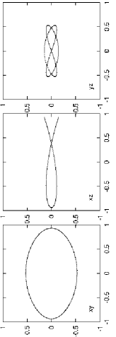
Figure 7: The 3D x2-like orbit x2mul2. This is a family of multiplicity 2.

reflecting the double multiplicity of the family, while the $(y,z)$ projection offers a shape that could produce a tiny boxy structure in the central region of the bar (note the scale on the axes). The $(x,z)$ projection can also offer a boxy structure, if one considers together with every orbit its symmetric with respect to the $z$ axis. This, however, is elongated along the minor axis of the bar as will be discussed in paper III. The morphology of this family shows that the model clearly can support in its face-on projection the presence of stellar rings in the x2-x3 area. This, however, is a thick ring structure extending outside the equatorial plane.

4.3 The main 3D families

The x1 S$\rightarrow$U transition at about $E_{j}\approx-0.36$ (Fig. 6b), generates the 3D family of periodic orbits x1v1. This family is related with the presence of the vertical 2:1 resonance. It has a stable part close to the bifurcating point, then it has a complex unstable part after an S$\rightarrow$$\Delta$ transition, and becomes again stable at about $E_{j}\approx-0.253$. We have found x1v1 as stable up to $E_{j}\approx-0.147$.

The morphological evolution of the family x1v1 is given in Fig. 8. This family corresponds to the z2 family of Hasan et al. (1993) and its orbits have been associated with the appearance of the peanut shaped bulges by Combes, Debbasch, Friedli et al. (1981). Indeed, due to the symmetry of the potential with respect to the equatorial plane, one can find all 3D families in pairs. Thus for x1v1 we will have the smile ($\smile$) and frown ($\frown$) types of the $(y,z)$ edge-on projections coexisting at a given energy, and the same holds for the $(x,z)$ projection. The $(x,y)$ projections of the 3D orbits follow in general the morphology of the corresponding x1 orbit of the same energy. As we said in the introduction, the importance of a family of stable periodic orbits is limited as the individual orbits grow in $|z|$. The x1v1 orbit for $E_{j}=-0.2$ in Fig. 8c exceeds both in its $(x,z)$ and its $(y,z)$ projections the height of 2 kpc and this means that it cannot contribute significantly to the density of the galactic disc. Its spatial extent on the other hand indicates that this orbit could be used to populate the bulge area.

The U$\rightarrow$S transition at $E_{j}\approx-0.343$ generates the family x1v2 which we followed until $E_{j}\approx-0.173$. It remains totally unstable and ends after a U $\rightarrow$ D $\rightarrow$ $\Delta$ sequence. It thus doesn’t play any important role in the dynamics of the system.

Family x1v3 (Fig. 9) is stable and its orbits keep low $|z|$ values roughly in the interval $-0.293<E_{j}<-0.221$. It then ends with a S$\rightarrow$$\Delta$ transition. This family is similar to the z1 family of Hasan et al. (1993). We note that both x1v1 and x1v3 provide useful orbits in the system before their S$\rightarrow$$\Delta$ transition. This behaviour is also seen in the 3D thick spiral model in Patsis & Grosbøl (1996). Complex instability helps introducing abrupt drops in the density of given features of a model (in our case the peanut), since it stops abruptly the existence of the family responsible for their appearance without bringing new stable families in the system. On the other hand, in cases where a stable family donates its stability to a bifurcation we have a smooth morphological evolution, which can give smooth density profiles in the galaxies. Both x1v1 and x1v3 do not have any intersections or tangencies with the $-2$ axis and for this reason they do not bifurcate other families with the same multiplicity.

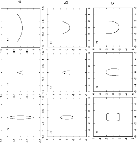
Figure 8: Three stable orbits of the x1v1 family. Note that the upper panels have a different scale than the middle and lower ones. Corotation in model A1 is at 6.13. The energies from top to bottom are: $E_{j}=-0.35$, $-0.25$ and $-0.20$ respectively.

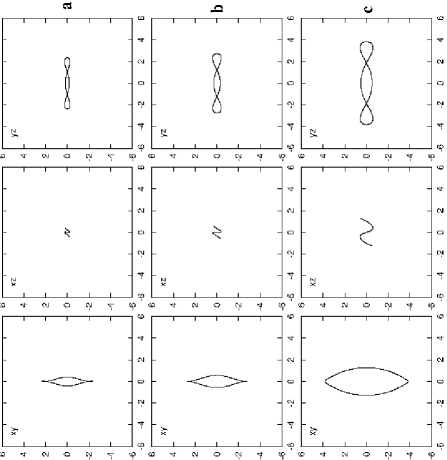
Figure 9: Three stable orbits of the x1v3 family. Their $(x,z)$ and $(y,z)$ projections have always low $|z|$ values. The energies from top to bottom are: $E_{j}=-0.28$, $-0.26$ and $-0.22$ respectively.

The next bifurcated family is x1v4. This is bifurcated from x1 after a U$\rightarrow$S transition. We would thus have expected it to be unimportant, since its parent family, x1, is unstable at the bifurcating point. This is the typical behaviour in such cases and we have seen it already happening for x1v2. x1v4 is introduced at about $E_{j}\approx-0.278$. One of the two stability indices, let us call it $b_{1}$, remains in the interval $-2<b_{1}<2$, while the other, $b_{2}$, goes to negative values smaller than $-2$. For larger $E_{j}$ values, however, $b_{2}$ increases and for about $E_{j}\approx-0.224$, both indices come in the stability zone, i.e. we have $-2<b_{1,2}<2$. The detailed description of this complicated evolution is beyond the scope of the present paper and does not add anything to the important information that family x1v4 brings stable representatives in the system for $E_{j}>-0.224$. The x1v4 family remains stable up to $E_{j}\approx-0.149$ where it becomes simple unstable. Its stability indices fold and the family continues existing towards smaller energies. The morphological evolution of x1v4 can be seen in Fig. 10. In Fig. 10a we give the three projections of an unstable orbit close to the bifurcating point from which the family emanates, while in Fig. 10b and

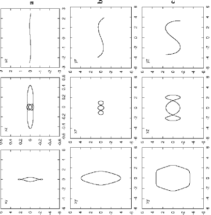
Figure 10: Orbits of the family x1v4. Panels (a) show an unstable orbit close to the bifurcating point at $E_{j}=-0.278$. Panels (b) and (c) show stable orbits for $E_{j}=-0.22$ and $E_{j}=-0.206$ respectively.

Fig. 10c we give two stable orbits, for energies $E_{j}>-0.224$. The last one is for $E_{j}=-0.206$ and we see that already the orbit reaches $|z|$ values close to 2 kpc away from the equatorial plane. For each orbit of this family there is also a symmetric one with respect to the equatorial plane. If only one of the two is populated, this would give rise to an asymmetric warp-like shape. Populating them both restitutes of course symmetry. The stable orbits of this family enhance the bar, but they deviate substantially from the equatorial plane.

4.4 Families at the 3:1 radial resonance

As we already saw, one of the two stability indices bifurcated the 3D families x1v1, x1v2, x1v3 and x1v4, by its intersections with the $b=-2$ stability axis. The intersections of the second stability index with this stability axis introduce in the system planar 2D orbits. The first family is bifurcated after a S$\rightarrow$U transition at $E_{j}\approx-0.244$, i.e. in the 3:1 resonance region. We call it t1 and it is stable (Fig. 11).

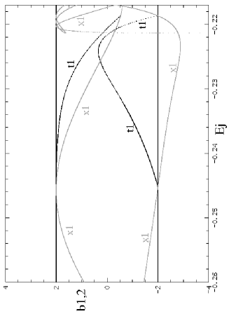
Figure 11: Stability diagram of the t1 family, the first radial bifurcation of x1 at the 3:1 resonance. The stability indices of x1 are given as well, drawn with light grey lines.

It bridges exactly the instability zone of the x1 in the S$\rightarrow$U$\rightarrow$S transition, i.e. its stability indices together with those of the x1, form a bubble [Contopoulos 1986]. t1 exists for approximately $-0.244<E_{j}<-0.218$ and at $E_{j}\approx-0.218$ can be considered as an inverse bifurcation of x1. At $E_{j}\approx-0.214$, just beyond the ‘bow’ area, the same stability index has another intersection with the $b=-2$ axis and x1 bifurcates another 2D family, t2. Several 2D and 3D 3:1 type families, related to each other and with x1, are introduced in the interval $-0.214<E_{j}<-0.20$. Let us briefly mention that, besides t1 (in Fig. 11) and t2, we found a third 2D 3:1 family, t3, which is stable for $-0.2065<E_{j}<-0.2005$, although it is introduced in the system as simple unstable for $E_{j}\approx-0.205$. The morphology of the three 2D families t1, t2 and t3 is given in Fig. 12, and their stable energy intervals in Table 3.

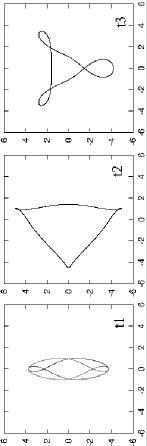
Figure 12: Stable orbits of the three 2-dimensional families at the 3:1 area. Note that the loops of t3 are asymmetric. In the left panel we plot a t1 orbit together with its symmetric with respect to the bar minor axis.

For the lower energies, the t1 orbits have only one loop, which is located on the $y$ axis, as the example shown in the left panel of Fig. 12. For higher energies they develop two more loops, symmetric with respect to the $y$ axis, and roughly equal in size to the first one. Since the orbits of family t1 are symmetric with respect to the $y$ axis, for every orbit we should have also its symmetric with respect to the $x$ axis. Combining the two, as in the left panel of Fig. 12, we obtain a shape that is elongated along the bar major axis and resembles the morphology of the x1 orbits with loops, at least for the energies where the orbits have only one loop. The extent of such orbits along the $y$ axis reaches up to 4 kpc, i.e. two thirds of the way to corotation.

t2 brings in the system three-dimensional families of periodic orbits with stable representatives. It bifurcates the family t2v1 at $E_{j}\approx-0.209$, which in turn bifurcates t2v1.1 at $E_{j}\approx-0.205$. The t2v1 family provides stable orbits to the system for $-0.209<E_{j}<-0.207$ and the t2v1.1 family for $-0.205<E_{j}<-0.203$. Triangular-like t2-type orbits have characteristic peaks at the sides of the bar, like the peak of the orbits at $x\approx-4$ in the $(x,y)$ projections of Fig. 13. They are near but not always on the minor axis of the bar and their presence can lead to local enhancements of the density at the area between the bar and the L_4,5 points.

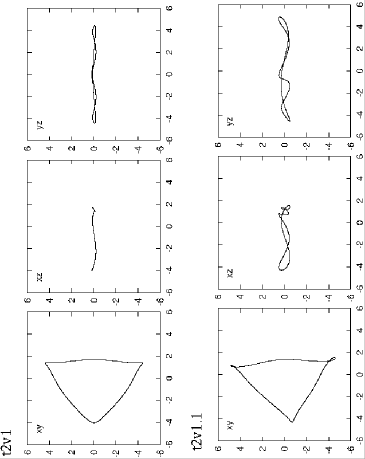
Figure 13: Stable orbits of two 3-dimensional families at the 3:1 area. Their names are given on the top left of each sets of panels.

For any energy in the interval $-0.214<E_{j}<-0.20$ there are almost always stable 3:1-type orbits of one or the other family. Together with t1, they affect the dynamics of the bar in this region. We note that the 3:1 orbits bifurcated from x1 are very common in all barred potentials and have both in 2D and 3D dynamically only local importance. Orbits of type t2v1 and t2v1.1 have been found even in the early $N$-body simulations of 3D bars (Figure 5 in Miller & Smith 1979). The loops of t3 on either side of the major axis of the bar are not of equal size. As can be seen by careful inspection of the t3 orbit in Fig. 12, the loop at the right side of the major axis is slightly bigger than the one to the left. Thus, morphologically, t3 is a kind of asymmetric t1, since for larger energies t1 develops loops which are symmetric with respect to the major axis, besides the one along the major axis.

4.5 The last part of the x1-tree

There are two more 3D bifurcations of x1 close to the local maximum of the characteristic at $E_{j}\approx-0.205$. It is x1v5 (bifurcated at $E_{j}\approx-0.213$ and being stable until $E_{j}\approx-0.172$) and x1v7 (bifurcated at $E_{j}\approx$ -0.205, just beyond the peak of the characteristic). The family x1v7 and its bifurcation x1v7.1 provide stable orbits for $-0.205<E_{j}<-0.18$ and $-0.175<E_{j}<-0.17$. Nevertheless, the part of this family that contributes to the density of the bar is limited by the fast increase of $|z|$ with the energy. Fig. 14 and 15 show the morphology of these families.

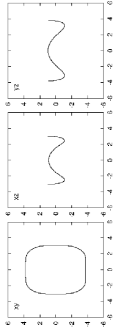
Figure 14: A typical stable x1v5 orbit.

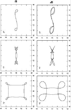
Figure 15: (a) A x1v7 orbit and (b) a x1v7.1 one. Both are stable.

In the same region we encounter two more 3D bifurcations of x1, namely the families x1v6, introduced at $E_{j}\approx-0.211$ (Fig. 4), and x1v8 introduced at $E_{j}\approx-0.1925$ (Fig. 5). Both are born after an U$\rightarrow$S transition of x1 and remain always unstable. We note that the representatives of x1v5, x1v6, x1v7 and x1v8 families are morphologically similar to those of the B$z_{2}$, B$\dot{z}_{2}$, B$\dot{z}_{3}$ and B$z_{3}$ families of Pfenniger (1984) respectively.

As we have seen, x1 is mostly unstable in the decreasing branch beyond the local maximum at the radial 4:1 gap and the morphology of the orbits at this branch is in general rectangular-like with loops in the corners. There are several families bifurcating from this branch and their orbits have, as already noted for other families, a morphology similar to that of x1 in the region. The 2D families q2 and q3 provide stable asymmetric orbits, two examples of which are given in Fig. 16. We also have one 3D bifurcating family, x1v9, a member of which is shown in Fig. 16. This family also has an asymmetric stable bifurcation for a short energy interval. No stable members of these families can be found outside the interval $-0.186<E_{j}<-0.1808$. To this we should add the small intervals of stability provided by x1 itself (cf. Fig. 1 and Fig. 5).

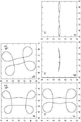
Figure 16: Morphology of stable orbits of x1’s bifurcations at largest energy values. Panels (a) and (b) show members of families q2 and q3 respectively. Panels (c) to (e) show the three views of an orbit of the x1v9 family.

Finally, for the sake of completeness we give in Fig. 17 the morphology of the three 3D families, members of the x1-tree, which remain always unstable although they exist for large energy intervals. As we have seen in the corresponding paragraphs they are the families x1v2, x1v6 and x1v8.

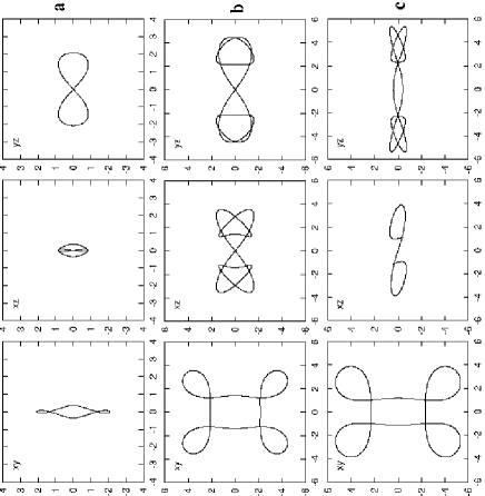
Figure 17: Orbits of the unstable families x1v2 (a), x1v6 (b), and x1v8 (c) at $E_{j}=-0.2612,\;-0.178$ and $-0.184$ respectively.

5 Further families

5.1 Orbits around L₄ and L₅

Another important ‘forest’ of families is the group of the banana like orbits. Here we find the usual planar long and short period banana-like orbits [Contopoulos & Grosbøl 1989]. The long period orbits are coming in the system in a large variety of families all of which have stable parts for $-0.1984<E_{j}<-0.1944$. The stability indices of these orbits exhibit a complicated behaviour having several tangencies and intersections with the $b=2$ and $b=-2$ axes. This brings many families in the system by bifurcation. The family found for lowest $E_{j}$ values is ban1 (Fig. 18a) which is born at $E_{j}\approx-0.1984$, followed by ban2 (Fig. 18b,c) that appears at a slightly greater energy value - which in turn bifurcates ban2.1 (Fig. 18d) at $E_{j}\approx-0.1972$ - and ban3 (Fig. 18e,f) introduced in the system at $E_{j}\approx-0.1983$. The most important of the planar orbits with stable parts, is ban4 (Fig. 18h), because it is stable over the largest energy interval ($-0.1982<E_{j}<-0.1955$). It exists for $E_{j}>-0.1982$ and it is not bifurcated at this point from any of the families existing for lower energies (ban1, ban2, ban2.1, ban3, ban3.1). From ban4 bifurcates the 2D family ban4.1 (Fig. 18g). The stability indices of ban4 have a complicated behaviour which is typical of a collision of bifurcations [Contopoulos 1986]. Approaching $E_{j}=-0.1955037765$, the ban4 orbits shrink to L₄ (or L₅), and beyond this point the short period orbits (spo) grow in size and take their bean-like shape (Fig. 18h and i respectively).

We have also found three 3D families of periodic orbits with stable parts. ban3v1 (Fig. 19a), a bifurcation of ban3 at $E_{j}\approx-0.1982$, is initially marginally stable, having one of its two stability indices almost equal to $-2$, but for $E_{j}>-0.1962$ the index become clearly larger than $-2$. At $E_{j}\approx-0.1947$ the two indices join each other and we have a S$\rightarrow$$\Delta$ transition. ban4v1 (Fig. 19b), a bifurcation of ban4 at $E_{j}\approx-0.1976$, is almost everywhere marginally stable in the interval $-0.1976<E_{j}<-0.1944$. For $E_{j}>-0.1944$ it is always complex unstable. ban3v1 and ban4v1 extend to very large $E_{j}$ values, but as complex unstable. Since we have S$\rightarrow$$\Delta$ transitions there are no bifurcating families and this is the mechanism that terminates the trapping of material around banana-like orbits in our 3D bars. Finally banv1 (Fig. 19c) is introduced in the system at $E_{j}\approx-0.1957$ as stable and remains stable up to $E_{j}\approx-0.1954$. This family is not obviously related to any other banana-like orbit. Since it is a 3D family we name it banv1.

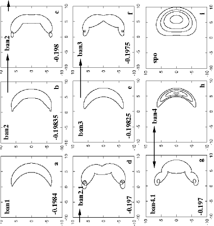
Figure 18: Stable 2D banana-like orbits. $E_{j}$ is given in the lower left corner of panels (a) to (g). Panels (h) and (i) include orbits of many $E_{j}$ values. Arrows indicate morphological evolution of the same or related families.

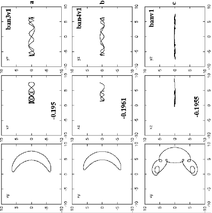
Figure 19: Stable 3D banana-like orbits. All three extend to large $E_{j}$ values but the two most important (ban3v1, ban4v1) are at these large $E_{j}$ values complex unstable. The numbers at the bottom of the $(x,z)$ projections give the $E_{j}$ of each orbit.

5.2 Orbits around L₁ and L₂

The L₁, L₂ Lagrangian points are known to be always unstable [Binney & Tremaine 1987]. Around them we find a family of planar periodic orbits we call $\ell_{1}$. It appears for $E_{j}$ values larger than the one corresponding to L₁, the morphology of its orbits resembles that of the spo orbits rotated by $\pi/2$, and their periods are of the order of the epicyclic period. Close to the L₁ energy and for $E_{j}<-0.168$ these orbits are unstable. For $E_{j}>-0.168$, however, $\ell_{1}$ has both stability indices between $-2$ and 2 and the family becomes stable. Orbits of this family can be found only by starting with initial conditions on the major axis of the bar. For this reason they had not been previously found, since in previous studies searches for periodic orbits started only with initial conditions on the $y=0$ axis. In Fig. 20, we plot a few stable orbits of $\ell_{1}$ and their symmetrics with respect to the $x$ axis for $E_{j}>-0.168$.

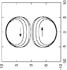
Figure 20: Stable orbits of the $\ell_{1}$ family and their symmetrics with respect to the $x$ axis. The innermost orbit, just next to the arrow, corresponds to $E_{j}\approx$ -0.168, just after the U$\rightarrow$S transition.

These stable orbits do not support the bar since they are elongated parallel to the minor axis. Nevertheless, they are of physical interest since they support motion parallel to the minor axis, contribute to the exchange of material between regions inside and outside corotation and are able to influence the dynamics in the region between bar and spirals in barred spiral galaxies. The streaming at the apocentra of the $\ell_{1}$ orbits could support arc-like features beyond the end of the bar.

For larger energies the $\ell_{1}$ orbits can be observed shifted towards the $x$ axis (minor axis of the bar), at about $E_{j}\approx-0.12$ they cross the $x$ axis and after a short unstable zone they fall on the retrograde family x4 as stable.

5.3 Orbits outside corotation

Beyond corotation we find the usual planar families [Contopoulos & Grosbøl 1989]. Most of their members display loops. We also find several 3D families with stable parts. As an example we give the family depicted in Fig 21, which is a bifurcation of the planar family called x1(1) by Contopoulos & Grosbøl (1989). The vertical extent of the 3D orbits we found beyond corotation is in general small.

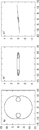
Figure 21: A 3D stable orbit beyond corotation.

Let us also mention some 2D families, orbits of which are given in Fig. 22. They have been calculated starting with initial conditions on the major axis of the bar as in the case of the $\ell_{1}$ family and have thus not been described in previous papers. All of them have large stable parts. These orbits have two interesting properties. First, some of them could support motion close to the end of the bar parallel to its minor axis, at radii shorter than the corotation radius. Second, they could efficiently transport material from the outer parts of the disc, e.g. from a distance close to 20 kpc from the center, to the central regions of the bar (e.g. Fig. 22a). This is particularly true for orbits as those shown in Fig. 22a and c.

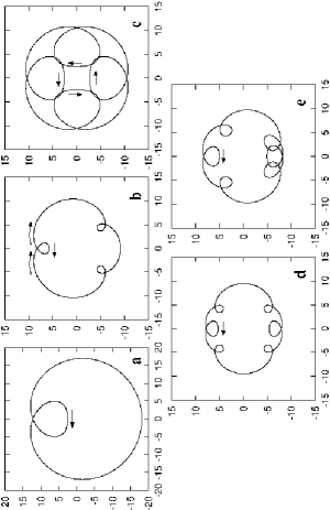
Figure 22: Examples of stable 2D orbits beyond corotation. They support motion parallel to the minor axis of the bar at the corotation region and favour exchange of material between regions far from the center and regions near to it.

6 Conclusions

In this paper we have made an extensive study of both the 2D and 3D periodic orbits in a fiducial model representative of a barred galaxy. We report on the stability and morphology of the main families. Our main conclusions are:

1. So far the x1 orbits were considered the backbone of bars. This, however, can only be the case for 2D bars, since the x1 can only populate the $z$=0 plane. For 3D bars the backbone is the x1, together with the tree of its 3D bifurcating families. Trapping around these families will determine the thickness and the vertical shape of galaxies in and around the bar region. Major building blocks for the 3D bars can be supplied also by families initially introduced as unstable. Thus the family x1v4, introduced in the system after a U$\rightarrow$S transition, is a basic family, giving stable representatives for large energy intervals in the system.

2. The $(x,y)$ projections of the 3D families of the x1-tree retain in general a morphological similarity with their parent family at the same energy. This has important implications for the morphology of a galaxy since it introduces building blocks which have similar morphology as the x1 orbits, but have a considerable vertical extensions. Especially at the regions close to the bifurcating points the $(x,y)$ morphology of a x1v$n$ family is not only geometrically similar, but actually very close to the morphology of the corresponding x1 orbit.

3. The way the 3D families of the x1-tree are introduced in the system at an instability strip determines the importance of the bifurcations in $z$ or $\dot{z}$. Particularly in the present model, all 3D families of the x1-tree at the increasing part of the characteristic which are bifurcated in $z$ are introduced in the system as stable. On the other hand the stable family associated with the 5:1 vertical resonance (x1v7), bifurcated at the decreasing part of the x1 characteristic, beyond its local maximum, is bifurcated in $\dot{z}$. Whether the stable family of the last S$\rightarrow$U$\rightarrow$S transition is the bifurcation in $z$ or $\dot{z}$ determines in a large degree the model’s morphology at its outer parts.

4. The radial 3:1 resonance region provides in the system several 2D and 3D stable families. Their role, however, is locally confined, as in 2D models.

5. 3D orbits elongated along the minor axis of the bar can be given by bifurcations of the planar x2 family.

6. We have found several families of 3D banana-like orbits around L_4,5. Their extent is always restricted by a S$\rightarrow$$\Delta$ transition.

7. Stable families found beyond corotation circulate material between the outer parts of the system and regions as far inwards as 1 kpc. This contributes to the mixing of the elements in a disc galaxy.

The families of periodic orbits we described up to now are indeed the basic families of a 3D Ferrers bar. As we explore the parameter space, however, their properties change, while new important families may appear and play a crucial role. A notable example is z3.1s, a family related to the z-axis orbits along the rotational axis, which will be described in paper II. However, these are rather particular cases and are not encountered in every model.

References

- [Athanassoula ] Athanassoula E., 1984 Phys. Rep. 114, 319
- [Athanassoula 1992a] Athanassoula E., 1992a, MNRAS 259, 328
- [Athanassoula 1992b] Athanassoula E., 1992b, MNRAS 259, 354
- [Athanassoula 1996] Athanassoula E., 1996, in ‘Spiral Galaxies in the near-IR’, D. Minniti & H.-W. Rix (eds.), p. 147, Springer
- [Athanassoula et al. 1983] Athanassoula E., Bienayme O., Martinet L., Pfenniger D., 1983, A&A 127, 349
- [Binney & Tremaine 1987] Binney J., Tremaine S., 1987, ‘Galactic Dynamics’, Princeton University Press, Princeton, N.J.
- [Broucke 1969] Broucke R., 1969, NASA Techn. Rep. 32, 1360
- [Combes et al. 1990] Combes F., Debbasch F., Friedli D., Pfenniger D., 1990, A&A 233, 95
- [Contopoulos 1980] Contopoulos G., 1980, A&A 81, 198
- [Contopoulos 1985] Contopoulos G., 1985, in ‘Chaos in Astrophysics’, J.R. Buchler et al (eds.), p. 259, Reidel
- [Contopoulos 1986] Contopoulos G., 1986, Celest. Mech. 38, 1
- [Contopoulos & Barbanis 1985] Contopoulos G., Barbanis B., 1985, A&A 153, 44
- [Contopoulos & Grosbøl 1988] Contopoulos G., Grosbøl P., 1988, A&A 197,83
- [Contopoulos & Grosbøl 1989] Contopoulos G., Grosbøl P., 1989, A&AR, 1,261
- [Contopoulos & Magnenat 1985] Contopoulos G., Magnenat P., 1985, Celest. Mech. 37, 387
- [Contopoulos & Mertzanides 1977] Contopoulos G., Mertzanides C., 1977, A&A 61, 477
- [Hadjidemetriou 1975] Hadjidemetriou J., 1975, Celest. Mech. 12, 255
- [Hasan, Pfenniger & Norman 1993] Hasan H., Pfenniger D., Norman C., 1993, ApJ 409, 91
- [Heggie 1985] Heggie D.C., 1985, Celest. Mech. 35, 357
- [Heisler et al. 1982] Heisler J., Merritt D., Schwarzschild M., 1982, ApJ 258, 490
- [Kormendy 1982] Kormendy J., 1982, in ‘Morphology and Dynamics of Galaxies’, L. Martinet and M. Mayor eds., 12th Advanced Course, Saas-Fee, p. 113, Geneva Obs., Sauverny
- [Martinet & Pfenniger 1987] Martinet L., Pfenniger D., 1987, A&A 173, 81
- [Martinet & de Zeeuw 1988] Martinet L., de Zeeuw T., 1988, A&A 206, 269
- [Miller & Smith 1979] Miller R.H., Smith B.F., 1979, ApJ 1979, 227, 785
- [Miyamoto & Nagai 1975] Miyamoto M., Nagai R., 1975, PASJ 27, 533
- [Olle & Pfenniger 1998] Olle M., Pfenniger D., 1998 A&A 334, 829
- [Patsis et al. 1997] Patsis P.A., Athanassoula E., Quillen A.C., 1997, ApJ 483, 731
- [Patsis & Grosbøl 1996] Patsis P.A., Grosbøl P., 1996, A&A 315, 371
- [Patsis et al. 2002] Patsis P.A., Skokos Ch., Athanassoula E., 2002 (paper III - in preparation)
- [Patsis et al. 2002] Patsis P.A., Skokos Ch., Athanassoula E., 2002 (paper IV - in preparation)
- [Pfenniger 1984] Pfenniger D., 1984, A&A 134, 373
- [Pfenniger 1985a] Pfenniger D., 1985a, A&A 150, 97
- [Pfenniger 1985b] Pfenniger D., 1985b, A&A 150, 112
- [Pfenniger 1987] Pfenniger D., 1987, A&A 180, 79
- [Pfenniger 1990] Pfenniger D., 1990, A&A 230, 55
- [Pfenniger 1996 ] Pfenniger D., 1996, in ‘Barred Galaxies’, ed. R. Buta, D. A. Crocker and B. G. Elmegreen, ASP Conf. Ser. 91, p.273
- [Poincaré 1899] Poincaré H, 1899, ‘Les Methodes Nouvelles de la Mechanique Celeste’, Vol III, Gauthier-Villars, Paris
- [Polymilis et al., 1997] Polymilis C., Servizi G., Skokos Ch., 1997, Celest. Mech. Dyn. Astron. 66, 365
- [Sellwood & Wilkinson 1993] Sellwood J., Wilkinson A., 1993, Rep. Prog. Phys. 56, 173
- [Schwarzschild, 1979] Schwarzschild M., 1979, ApJ 232,236
- [Skokos 2001] Skokos Ch., 2001, Physica D 159, 155
- [Skokos et al. 2002] Skokos Ch., Patsis P.A., Athanassoula E., 2002 MNRAS - this issue
Acknowledgments
We acknowledge fruitful discussions and very useful comments by Prof. G. Contopoulos. We thank the referee for useful suggestions that allowed to improve the presentation of our work. This work has been supported by EET II and K 1994-1999; and by the Research Committee of the Academy of Athens. Ch. Skokos and P.A. Patsis thank the Laboratoire d’Astrophysique de Marseille for an invitation during which essential parts of this work have been completed.