Phase Mixing in Unperturbed and Perturbed Hamiltonian Systems

Abstract

This paper summarises a numerical investigation of phase mixing in time-independent Hamiltonian systems that admit a coexistence of regular and chaotic phase space regions, allowing also for low amplitude perturbations idealised as periodic driving, friction, and/or white and colored noise. The evolution of initially localised ensembles of orbits was probed through lower order moments and coarse-grained distribution functions. In the absence of time-dependent perturbations, regular ensembles disperse initially as a power law in time and only exhibit a coarse-grained approach towards an invariant equilibrium over comparatively long times. Chaotic ensembles generally diverge exponentially fast on a time scale related to a typical finite time Lyapunov exponent, but can exhibit complex behaviour if they are impacted by the effects of cantori or the Arnold web. Viewed over somewhat longer times, chaotic ensembles typical converge exponentially towards an invariant or near-invariant equilibrium. This, however, need not correspond to a true equilibrium, which may only be approached over very long time scales. Time-dependent perturbations can dramatically increase the efficiency of phase mixing, both by accelerating the approach towards a near-equilibrium and by facilitating diffusion through cantori or along the Arnold web so as to accelerate the approach towards a true equilibrium. The efficacy of such perturbations typically scales logarithmically in amplitude, but is comparatively insensitive to most other details, a conclusion which reinforces the interpretation that the perturbations act via a resonant coupling.

]

I INTRODUCTION AND MOTIVATION

Phase mixing is a fundamental process acting in many-particle systems, with important implications for a variety of different areas of physics extending from galactic dynamics[1] to the physics of charged particle beams[2]. In response to external forces and/or self-consistent interactions, initially localised collections of particles often tend to disperse. Phase mixing is believed to play a fundamental role in so-called “violent relaxation,” the process whereby the stars in an elliptical galaxy evolve towards a statistical meta-equilibrium and, under certain circumstances, it can play a major role in the dissipation of accelerator beams, resulting in substantial – and undesireable – increases in emittance.

Until recently, most practical considerations of phase mixing have assumed, at least implicitly, that the global dynamics is integrable or near-integrable, in which case initially localised ensembles typically disperse as a power law in time. However, there is emerging evidence that, in at least some settings relevant to galactic astronomy[3] and accelerator dynamics[4], one is confronted with strongly nonintegrable chaotic dynamics. The manifestations of phase mixing in chaotic systems are very different from those in nearly integrable systems[5], a fact which has led galactic astronomers to speak of a new phenomenon called chaotic mixing[6]. It is, e.g., obvious that localised ensembles of chaotic orbits will typically disperse exponentially rather than as a power law in time. For this reason, it would seem important to re-examine the physics of phase mixing, allowing explicitly for systems that admits large measures of chaos.

Of especial interest are the potential implications of chaotic phase space mixing for relaxation towards a statistical equilibrium or near-equilibrium. By reformulating the dynamics of a time-independent Hamiltonian system as a geodesic flow, e.g., using Maupertuis’ Principle[7], some rigorous mathematical results have been derived. For example, it is known that initially localised ensembles of geodesics on a compact manifold with constant negative curvature exhibit a coarse-grained approach, exponential in time, towards a uniform population of the manifold, i.e., a microcanonical distribution, at a rate ${\lambda}$ that is fixed completely by the magnitude of the curvature[8]. This implies the existence of a direct connection between ${\lambda}$ and the positive Lyapunov exponent(s) ${\chi}$. If the curvature is always negative but not constant, the flow becomes significantly more complex, but one can still infer an exponential approach towards a microcanonical equilibrium at a rate that is bounded from below by the least negative value of the curvature[9].

However, these results are of limited applicability to real physical systems where the curvature can vary in sign and, in many cases, may be strictly positive[10]. In such systems, it would appear[11] that chaos should be attributed to parametric instability rather than to negative curvature, the division of a constant energy hypersurface into chaotic and regular regions reflecting properties of the local curvature which do, or do not, trigger an instability. Within a suitably defined connected chaotic phase space region, ensembles may still relax exponentially towards a microcanonical population[5], but there is no reason to expect a one-to-one connection between the rate ${\lambda}$ and the Lyapunov exponents ${\chi}$.

Additional complications can also arise when the bulk dynamics is impacted significantly by phase space structures like cantori or an Arnold web[12]. If a connected chaotic phase space region is partitioned by such entropy barriers, i.e., phase space obstructions which impede, but do not completely block, orbital motions, phase space transport can entail a multi-stage process characterised by two or more vastly different time scales. In analogy with the classical problem of effusion of gas through a tiny hole, particles starting on one side of a barrier can evolve towards a near-uniform population of the phase space region on that side on a time scale $t_{s}$ much shorter than the time scale $t_{l}$ on which particles breech the barrier. On intermediate time scales, $t_{s}{\;}{\ll}{\;}t{\;}{\ll}{\;}t_{l}$, each side may be in a near-equilibrium but the densities on the two sides will in general be very different.

Significantly, however, even very small perturbations can accelerate phase space transport through such barriers. It has been long known from the study of maps[13] that small random perturbations, i.e., noise, can dramatically reduce the time scale for diffusion through cantori. And similarly, it has been recognised that even very low amplitude periodic driving can have important implications for phase space transport in systems like plasmas[14]. Recent work on continuous Hamiltonian systems[15, 16] has served to quantify this effect, demonstrating that weak noise and/or periodic driving can significantly impact phase space transport on time scales much shorter than the relaxation time $t_{R}$ on which they significantly change the values of quantities like energy, which would be conserved absolutely in the absence of perturbations. All this would suggest that low amplitude perturbations can significantly impact the phase mixing of chaotic orbits, a possibility that has direct physical implications for the destabilisation of various structures in a galaxy[17] or the defocusing of an accelerator beam[18].

This paper presents the results of a systematic numerical investigation of phase mixing for two- and three-degrees-of-freedom Hamiltonian systems that admit a complex coexistence of regular and chaotic phase space regions, allowing also for the effects of low amplitude perturbations idealised as periodic driving and/or friction and (in general coloured) noise.

In principle, one might argue that such an analysis is not completely applicable to real many-body systems where the dimensionality of the true phase space is much larger. However, there are at least three reasons to believe that the analysis summarised in this paper should find direct physical applications.

1. In a variety of physical systems, e.g., relatively low intensity beams[2] or stars in the center of a galaxy orbiting close to a supermassive black hole, one expects that the bulk properties of the flow will be dominated by ‘external’ bulk forces rather than self-interactions; and, to the extent that self-interactions are important, one might hope to model their effects as friction and noise in the context of a Fokker-Planck description.

2. Recent integrations of gravitationally interacting test particles in fixed, time-independent $N$-body realisations of smooth density distributions have shown that, at least for large $N$, these particles behave in a fashion closely resembling the motions of particles evolved in the corresponding smooth density distribution; and that the differences that do exist decrease with increasing $N$[19, 20, 21]. Moreover, in terms of both the statistical properties of individual orbits and the phase mixing of orbit ensembles, discreteness effects are extremely well mimicked by (a suitably defined) Gaussian white noise[21].

3. Performing honest $N$-body integrations of interacting systems for very large $N$ is not viable using current computational resources. However, fully self-consistent grid code simulations of intense charged beams have been found to exhibit both regular and chaotic phase mixing qualitatively similar to what has been found in smooth two- and three-dimensional potentials[4, 22].

White noise appears to be very successful in modelling discreteness effects in $N$-body systems, where the time scale on which the ‘random’ forces change is extremely short. However, real systems are also subjected to other, more slowly varying, perturbations which, in many cases, one might hope to model as (i) periodic driving and/or (ii) coloured noise with a finite autocorrelation time, i.e., ‘random’ forces that only change significantly on macroscopic time scales.

In the context of galactic astronomy, periodic driving could reflect the effect of companion galaxies, such as the Small and Large Magellanic Clouds orbiting the Milky Way. Viewed mathematically, coloured noise is a superposition of periodic perturbations combined with random phases. One might, therefore, use coloured noise to model a high density cluster environment, in which, over the course of time, the perturbations acting on any given galaxy result from complex interactions with a variety of different neighbouring galaxies. Alternatively, coloured noise might be used to model discrete substructures like molecular clouds or globular clusters, where the interaction time scale is too long to justify a white noise approximation.

Such perturbations may also influence the dynamics of charged-particle beams. In a cyclotron or synchrotron, irregularities in the confining and/or focusing magnetic fields would, from the perspective of the beam, appear as quasi-periodic perturbations with, perhaps, a slowly varying frequency. The conceptual paradigm for such beams is the Hénon-Heiles potential, $V(x,y)={1\over 2}(x^{2}+y^{2}+2x^{2}y-{2\over 3}y^{3})$, although in general detailed particle tracking is necessary for determining the effective, or ‘dynamic’, aperture of the machine. The same is true conceptually for linear accelerators comprising a periodic array of quadrupole and/or solenoid magnets. For beams wherein the self-field, i.e., space charge, is active, in general the situation is more complicated. Transitions in the focusing force can lead to dynamics similar to violent relaxation in stellar systems, i.e., the presence of a hierarchy of collective modes or, for large transitions, correlations analogous to plasma turbulence. Other processes, such as beam generation at the source, or bunch compression, may impose irregularities in the form of microstructure, i.e., density correlations, on the beam. Space-charge forces from these ‘clumps’ may influence individual particle orbits in the manner of colored noise.

Considerations such as these imply that the microscopic dynamics of beams and stellar systems are linked, a point that, until recently, seems to have been overlooked in the literature. The specific mechanism that connects these diverse systems is phase mixing.

Section II of this paper describes the models that were considered and the numerical experiments that were performed. Section III then summarises the results obtained for unperturbed Hamiltonian systems. Section IV describes how these results are alterred in the presence of friction and white noise, which might be expected to mimic discreteness effects in a many-body system. Section V considers in turn the effects of periodic driving and/or coloured noise with a finite autocorrelation time, which might be expected to mimic systematic and/or near-random perturbations that cannot be modeled as instantaneous kicks. Section VI summarises the principal conclusions and comments on potential applications.

II THE EXPERIMENTS PERFORMED

The research described here focused on two- and three-degrees-of-freedom Hamiltonian systems of the form

$$H={1\over 2}\left(v_{x}^{2}+v_{y}^{2}+v_{z}^{2}\right)+V(x,y,z).$$ (1)

Three different classes of potential were considered. The simplest, which appears to exhibit comparatively generic behaviour[23], is a straightforward generalisation of the two-degrees-of-freedom dihedral potential[24], allowing for three free parameters, $a$, $b$, and $c$:

$$V(x,y,z)=-x^{2}-y^{2}-z^{2}+{1\over 4}\left(x^{2}+y^{2}+z^{2}\right)^{2}$$

$$-{1\over 4}\left(ax^{2}y^{2}+by^{2}z^{2}+cz^{2}x^{2}\right).$$ (2)

The second is given as a combination of isotropic and anisotropic Plummer potentials[25]:

$$\hskip-36.135ptV(x,y,z)=-{1\over(a^{2}+x^{2}+y^{2}+z^{2})^{1/2}}$$

$$\hskip 36.135pt-{m\over(a^{2}+x^{2}+b^{2}y^{2}+c^{2}z^{2})^{1/2}}.$$ (3)

For generic choices of parameters $a$, $b$, $c$, and $m$ and ‘reasonable’ choices of energy $E$, both these potentials yield phase space hypersurfaces admitting a complex coexistence of both regular and chaotic orbits.

The third potential is the sum of two integrable contributions, an anisotropic harmonic potential and an isotropic Plummer potential[26]:

$$V(x,y,z)={1\over 2}(a^{2}x^{2}+b^{2}y^{2}+c^{2}z^{2})-{M\over\sqrt{r^{2}+{\epsilon}^{2}}},$$ (4)

with $r^{2}=x^{2}+y^{2}+z^{2}$ . This potential is interesting in the sense that, provided that $M$ is not too large, chaotic orbits with positive Lyapunov exponent only exhibit strong exponential sensitivity for the small fraction of time they are at comparatively small $r$[27]. At larger $r$ the motions are ‘nearly regular.’

Two-degree-of-freedom systems were obtained trivially by considering orbits with initial conditions $z{\;}{\equiv}{\;}v_{z}{\;}{\equiv}{\;}0$.

Results derived for motion in the unperturbed potentials were contrasted with motions subjected to two different classes of perturbations:

1. Periodic driving. This entailed either allowing for a simple sinusoidal driving, resulting in evolution equations of the form

$${d^{2}r_{i}\over dt^{2}}=-{{\partial}V\over{\partial}r_{i}}+A_{i}\sin\,{\omega}_{i}t\qquad(i=x,y,z),$$ (5)

or introducing systematic oscillations in one or more of the constants in the unperturbed potential, e.g., considering a perturbed version of eq. (2.3) with

$$a\to a_{0}(1+\sin\,{\omega}t)\;\;\;{\rm or}\;\;\;m\to m_{0}(1+\sin\,{\omega}t),$$ (6)

or

$$V({\bf r},t)\to\left(1+A\sin{\omega}t\right)\times V({\bf r}),$$ (7)

2. Friction and noise. This entailed considering Langevin equations of the form

$${d^{2}r_{i}\over dt^{2}}=-{{\partial}V\over{\partial}r_{i}}-{\eta}{dr_{i}\over dt}+F_{i}\qquad(i=x,y,z),$$ (8)

which incorporate a dynamical friction $-{\eta}dr_{i}/dt$ and a pseudo-random force $F_{i}$, idealised as Gaussian noise with zero mean. The friction and noise were typically taken to be related by a Fluctuation-Dissipation Theorem

$${\langle}F_{i}(t_{1})F_{j}(t_{2}){\rangle}=K(t_{1}-t_{2}){\delta}_{ij}$$ (9)

with diffusion constant

$$D=\int_{-\infty}^{\infty}d{\tau}K({\tau})=2{\eta}{\Theta},$$ (10)

in terms of a ‘temperature’ ${\Theta}{\;}{\sim}{\;}|E|$. Three forms of noise were considered, namely:

${\bullet}$ white noise, which is delta-correlated in time, with

$$K({\tau})=2{\Theta}{\eta}{\delta}_{D}({\tau}),$$ (11)

${\bullet}$ coloured noise sampling an Ornstein-Uhlenbeck process, for which the autocorrelation function

$$K({\tau})={\alpha}{\eta}{\Theta}\exp(-{\alpha}|{\tau}|),$$ (12)

corresponding to an autocorrelation time $t_{c}=1/{\alpha}$, and

${\bullet}$ coloured noise characterised by a more complex autocorrelation function

$$K({\tau})={3{\alpha}{\eta}{\Theta}\over 8}\exp(-{\alpha}|{\tau}|)\left(1+{\alpha}|{\tau}|+{{\alpha}^{2}\over 3}{\tau}^{2}\right),$$ (13)

for which $t_{c}=2/{\alpha}$. The white noise autocorrelation function (2.10) can be derived from either (2.11) or (2.12) in a singular limit ${\alpha}\to\infty$. White noise was implemented numerically using a standard algorithm[28]. Coloured noise was implemented using an algorithm developed by I. V. Pogorelov as part of his Ph. D. dissertation[29].

Phase mixing was investigated by tracking the evolution of localised ensembles of $N$ initial conditions of fixed energy $E$, with $1600{\;}{\leq}{\;}N{\;}{\leq}{\;}40000.$ These were typically generated by uniformly sampling a four- or six-dimensional phase space hypercube of side ${\Delta}Z$, with ${\Delta}Z{\;}{\sim}{\;}10^{-3}$ the size of the accessible phase space region. The initial conditions were integrated using a standard integration scheme which simultaneously tracked the evolution of a small initial perturbation, periodically renormalised in the usual way[12], so as to extract estimates of the largest (finite time) Lyapunov exponent.

Two diagnostics were used to probe the evolution of each ensemble:

${\bullet}$ lower order moments of the form

$${\langle}x^{A}y^{B}z^{C}v_{x}^{D}v_{y}^{E}v_{z}^{F}{\rangle}\qquad A+B+C+D+E+F{\;}{\leq}{\;}6,$$ (14)

computed in the obvious way; and

${\bullet}$ coarse-grained two-dimensional distribution functions like $f(x,y,t)$ or $f(x,v_{x},t)$, generated by gridding the orbital data at fixed instants of time into a $k\times k$ grid with $k$ ranging between $5$ and $40$.

The initial divergence of an ensemble was probed by tracking the rate at which quantities like the dispersions ${\sigma}_{x}$ or ${\sigma}_{v_{x}}$ grow. The approach towards an equilibrium or near-equilibrium was probed by tracking (i) the convergence of various moments towards time-independent ‘equilibrium’ values and (ii) the evolution of coarse-grained distributions towards a nearly time-independent form. For example, it is an empirical fact that, in each potential, chaotic ensembles typically evolve towards a state in which, modulo finite-$N$ statistics, ${\langle}x{\rangle}=0$ and ${\sigma}_{x}$ assumes a constant value ${\sigma}_{x0}$. The obvious question, then, is whether the decay of ${\langle}x(t){\rangle}$ and $D{\sigma}_{x}(t){\;}{\equiv}{\;}{\sigma}_{x}(t)-{\sigma}_{x0}$ towards zero is power law or exponential, and, for the case of chaotic ensembles, the degree to which the rates associated with this decay correlate with the finite time Lyapunov exponents of the orbits.

Convergence of coarse-grained distributions was handled analogously[5]. Motivated by the visual impression that, at least for chaotic ensembles, the orbits usually approach a nearly time-independent equilibrium state, the last $q$ snapshots of a sequence of $p$ snapshots can be used to derive a near-invariant distribution

$$f_{niv}(Z_{i},Z_{j})={1\over q}\sum_{p-q+1}^{p}f(Z_{i},Z_{j},t_{q}),$$ (15)

and convergence towards $f_{niv}$ can then be probed by computing discretised $L^{p}$ norms

$$D^{p}f(Z_{i},Z_{j},t)=\left(\sum\sum|f(Z_{i},Z_{j},t)-f_{niv}(Z_{i},Z_{j})|^{p}\over\sum\sum|f_{niv}({Z_{i},Z_{j})|^{p}}\right)^{1/p}$$ (16)

for $p=1$ and $2$, with sums extending over the $k\times k$ grid.

III UNPERTURBED HAMILTONIAN SYSTEMS

A Phase mixing of regular ensembles

Localised ensembles of initial conditions corresponding to regular orbits will, when evolved into the future, diverge as a power law in time. In particular, quantities like the dispersion ${\sigma}_{x}$ will typically grow linearly in time until they become comparable in magnitude to the size of the phase space region sampled by individual orbits in the ensemble.

This power law divergence is easily understood. Motion in the $x$- (or any other) direction is periodic, so that, after a period ${\tau}_{x,i}=2{\pi}/{\omega}_{x,i}$ each orbit $i$ will return to its initial value $x_{0,i}$. In general, however, the periods ${\tau}_{i}$ for nearby orbits will be slightly different, so that when orbit $i$ has returned to $x_{0,i}$, a slightly displaced orbit $j$ with different ${\tau}_{j}$ will not have returned to its initial $x_{0,j}$. It will instead assume a slightly different value $x_{j}$ which, on the average, is slightly further away from $x_{0,i}$ than the initial $x_{0,j}$. On the average, the two orbits will have moved further apart. (For the special case of a harmonic potential, where all the orbits have the same frequencies, there is no phase mixing.)

Let $t_{cr}{\;}{\sim}{\;}1/{\omega}$ denote a typical periodicity, ${\delta}{\tau}{\;}{\sim}{\;}1/{\delta}{\omega}$ a characteristic ‘spread’ in periodicities, and $R$ the linear ‘size’ of the configuration space region that is accessible to the orbits in the ensemble. The preceding argument then suggests that ${\sigma}_{x}$ should grow in such a fashion as to satisfy ${\sigma}_{x}/R{\;}{\sim}{\;}({\delta}{\omega})t.$ Presuming, however, that ${\delta}{\omega}{\;}{\sim}{\;}{\omega}{\Delta}/R$, where ${\Delta}$ is the ‘size’ of the region from which the initial conditions were derived, it follows that

$${\sigma}_{x}(t){\;}{\sim}{\;}(t/t_{reg})R,\;\;{\rm with}\;\;t_{reg}({\Delta}){\;}{\sim}{\;}(R/{\Delta})t_{cr}$$ (17)

or, equivalently,

$${\sigma}_{x}(t){\;}{\sim}{\;}{\Delta}\,(t/t_{cr}).$$ (18)

That ${\sigma}_{x}$ grows linearly in time and that, at least approximately, ${\sigma}_{x}{\;}{\propto}{\;}{\Delta}$ and $t_{reg}{\;}{\propto}{\;}1/{\Delta}$ are both illustrated in Fig. 1, the first five panels of which track ${\sigma}_{x}(t)$ for ensembles of initial conditions evolved in the two-dimensional dihedral potential with $a=1$ and energy $E=2.0$. In each case, a cell of $20000$ initial conditions was constructed, centered about a fixed phase space point $(x_{0},y_{0},v_{x,0},v_{y,0})$. The ensembles were generated by setting $v_{y}=v_{y,0}$, uniformly sampling a configuration space square of size ${\Delta}$, and, for each choice of $x$ and $y$, solving for $v_{x}=v_{x}(E,x,y,v_{y})>0$. The five panels correspond to values ranging from ${\Delta}=1.0\times 10^{-3}$ to ${\Delta}=5.0\times 10^{-2}$. The sixth panel exhibits on a log-log plot the best fit growth time $t_{reg}$ as a function of ${\Delta}$. The best fit value for the slope is $p=-0.95$, which implies a scaling $t_{reg}{\;}{\propto}{\;}{\Delta}^{-0.95}$. A dashed line corresponding to slope $p=-1$ is shown for comparison. Given that, for this potential and energy, $t_{cr}{\;}{\sim}{\;}5-10$ and $R{\;}{\sim}{\;}1$, the amplitude of $t_{reg}({\Delta})$ is also consistent with eq. (3.1).

When integrated for much longer times, regular ensembles typically exhibit a coarse-grained evolution towards an invariant equilibrium distribution. This reflects the fact that, over very long times, individual regular orbits will, in a time-averaged sense, tend to uniformly populate the KAM tori to which their motions are restricted.

This convergence can be quantified by tracking the evolution of lower order moments for the ensemble, which eventually converge towards equilibrium values. Examples thereof are exhibited in the first four panels of Fig. 2, which were generated from the same ensembles used to create Fig. 1d and e. These correspond to collections of regular ‘box’ orbits, with the configuration space topology of Lissajous figures. The invariant distributions associated with these ensembles are symmetric with respect to reflection about the $x$- and $y$-axes and, as such, have moments ${\langle}x{\rangle}_{inv}={\langle}y{\rangle}_{inv}=0$.

It is evident that ${\langle}x(t){\rangle}$ is indeed converging towards zero, but that the time scale associated with the convergence is very long. Also evident is the fact that the time dependence of ${\langle}x{\rangle}$ is comparatively complex: Strictly speaking, the evolution is neither exponential nor power law in time; and, even at very late times, $t>4000$, one can see coherent evolutionary effects reflecting the fact that the orbits all have well-defined periodicities.

One final point is also clear. Just as the size ${\Delta}$ determines the time scale on which ensembles disperse initially, so also ${\Delta}$ fixes the time scale on which they evolve towards an equilibrium. For the ensemble exhibited in panels Figs. 2a and b, ${\Delta}$ is $2.5$ times larger than for the ensemble exhibited in Figs. 2c and d, so that, as illustrated in Fig. 1, the first ensemble disperses approximately $(2.5)^{0.95}{\;}{\approx}{\;}2.38$ times as fast. However, by replotting in panels e and f the data for Fig. 2a and b over the shorter interval $T=(8000/2.38){\;}{\approx}{\;}3360$, it becomes evident visually that the first ensemble also approaches an equilibrium approximately $2.38$ times as fast.

B Phase mixing of chaotic ensembles

Initially localised ensembles of chaotic orbits evolve very differently. Considerable variability can be observed but, overall, chaotic ensembles tend to disperse exponentially at a rate ${\Lambda}{\;}{\equiv}{\;}t_{cha}^{-1}$ that is comparable to the largest positive Lyapunov exponent ${\chi}$. Thus, e.g.,

$${\sigma}_{x}{\;}{\sim}{\;}{\Delta}\,\exp(t/t_{cha})\qquad{\rm with}\qquad t_{cha}{\;}{\sim}{\;}{\chi}^{-1},$$ (19)

with ${\Delta}$ the ‘size’ of the cell of initial conditions. This exponential growth implies that chaotic phase mixing is typically much faster than regular phase mixing.

The physics of chaotic phase mixing is very different from the phase mixing of regular ensembles. Aperiodic chaotic orbits exhibit exponentially sensitive dependence, so that two nearby initial conditions separated by some phase space distance ${\delta}Z_{0}$ will, when evolved into the future, typically diverge exponentially at a rate that is set by a Lyapunov exponent: ${\delta}Z(t){\;}{\sim}{\;}{\delta}Z_{0}\exp({\chi}t)$. Applying this principle to the ensemble as a whole leads immediately to eq. (3.3).

The appropriate ${\chi}$ entering into eq. (3.3) is a finite time Lyapunov exponent[30] appropriate for orbits in the ensemble for the interval associated with the exponential divergence, not the asymptotic Lyapunov exponent, as defined in a $t\to\infty$ limit, which can be very different. Two different ensembles that rapidly spread to occupy the same phase space region might be expected to have comparable ${\chi}$’s and to mix at comparable rates. However, it is possible for different ensembles, each in principle able to access the same phase space region, to have different finite time ${\chi}$’s and to mix at very different rates.

If the dispersal of the ensemble be probed in a generic direction, $t_{cha}^{-1}$ will typically be comparable to the largest positive (finite time) Lyapunov exponent. In general, a conservative nonintegrable potential in $D$ dimensions has $D-1$ unequal positive Lyapunov exponents, corresponding to $D-1$ different unstable directions. However, the rate at which an ensemble disperses in a specified phase space direction will be dominated by the Lyapunov exponent associated with the most unstable direction with a nonzero projection in that specified direction; and that most unstable direction will typically have a nonzero projection in a generic,‘randomly chosen’ direction[31].

It is, however, possible for certain directions to mix much more rapidly than others. As an extreme example, consider a three-dimensional potential where motion in (say) the $z$-direction is integrable and decoupled from chaotic motion in the two orthogonal directions. In this case, quantities like ${\sigma}_{z}$ and ${\sigma}_{v_{z}}$ will exhibit behaviour appropriate for regular phase mixing whereas quantities like ${\sigma}_{x}$ or ${\sigma}_{v_{y}}$ will in general exhibit the exponental behaviour predicted by eq. (3.3).

Individual chaotic orbits evolved in a generic potential can be impacted significantly by such topological obstructions as cantori and/or Arnold webs[12], which serve as entropy barriers to impede – but not block – motion between different portions of the same connected phase space region. If, however, the motions of individual members of an ensemble are impeded, the phase mixing of the ensemble as a whole will in general be alterred.

As a simple example, consider an ensemble of initial conditions corresponding to chaotic orbits which, at early times, are trapped near a regular island by cantori. The largest finite time Lyapunov exponents for such ‘sticky’[32] chaotic orbits will in general be substantially smaller than the exponents for ‘wildly chaotic’ orbits not trapped near regular islands[33]; and this implies that the ensemble will disperse more slowly than a ‘wildly chaotic’ ensemble. Even more significant, however, is the fact that, until the orbits have escaped through the cantori, quantities like ${\sigma}_{x}$ may remain much smaller in magnitude than the asymptotic value ${\sigma}_{x,\infty}$ towards which the ensemble converges at late times.

Representative data for a ‘wildly chaotic’ ensemble are exhibited in the left panels of Fig. 3, the upper curves in which exhibit ${\sigma}_{x}$, ${\sigma}_{y}$, and ${\sigma}_{z}$ for an ensemble evolved in the potential (2.4) with $a=1.95$, $b=1.50$, $c=1.05$, and $M=0.0316$. These curves show considerable short time structure but it is evident that, overall, the dispersions grow exponentially until they saturate on a scale comparable to the size of the accessible configuration space region. The exponential growth becomes especially apparent if the data are smoothed via box-car averaging. The lower curves in these panels, translated downwards by a distance $\ln{\sigma}=3.0$, illustrate the effect of averaging the raw data, recorded at intervals ${\delta}t=0.25$, over $20$ adjacent points. It is apparent visually that the growth rates associated with ${\sigma}_{x}$ and ${\sigma}_{y}$ are essentially identical. The behaviour in the $z$-direction is noticeably different, but the overall growth rate remains comparable.

Fig. 4 exhibits dispersions for chaotic ensembles evolved in the potential (2.2) with $a=b=c=1$. In each case, data were recorded at intervals ${\delta}t=0.5$, and the curves generated by box-car averaging over 5 adjacent points. Panels a and b present, respectively, smoothed configuration and velocity space dispersions for a ‘wildly chaotic’ ensemble with $E=1.0$, with the $y$- and $z$-components translated downwards by, respectively, $\ln{\sigma}=5$ and $10$. The dots surrounding the top curves represent unsmoothed data. It is evident that, for this ensemble, all six dispersions grow exponentially at comparable rates. Panel c presents configuration space dispersions for a ‘sticky’ ensemble with $E=4.0$. In this case, one still identifies an initial exponential growth, but that growth slows for $\ln{\sigma}>-1.0$ or so, and the eventual approach towards a near-invariant ${\sigma}_{0}$ is accompanied by oscillations not observed in most ‘wildly chaotic’ ensembles. Panel d exhibits exhibits configuration space dispersions for a particularly unusual example, in which dispersal in the $z$-direction is much slower than in the $x$- and $y$-directions. This anomalous behaviour reflects the fact that the cell of initial conditions was concentrated near the $x-y$ plane, where ${\partial}V/{\partial}z=0$.

Atypical behaviour is especially common for potentials like (2.4), where chaotic orbits behave in a nearly regular fashion ‘most of the time.’ It is, e.g., easy to identify ensembles which, at least initially, avoid the ‘highly chaotic’ central region and, as such only mix on comparatively long time scales. And, similarly, it is easy to construct ensembles which, because of the (initial) orbital orientations in the central regions, are considerably more chaotic in some phase space directions than in others.

As a clear example, one can contrast the data for the ‘wildly chaotic’ ensemble exhibited in the left panels of Fig. 3 with the right hand panel, which exhibits data for a different, much less chaotic, ensemble evolved in the same potential with the same energy. For the left ensemble, the mean value of the largest finite time Lyapunov exponent at $t=256$ is ${\langle}{\chi}{\rangle}{\;}{\approx}{\;}0.055$; for the right ensemble, ${\langle}{\chi}{\rangle}{\;}{\approx}{\;}0.022$. It is clear that, overall, the dispersions grow more rapidly for the wildly chaotic ensemble. Overlaying plots for the two ensembles also reveals another significant point: Although the sticky ensemble originally diverges more slowly, the rates of divergence become comparable when $\ln{\sigma}_{x}>-2$, the growth rate for the sticky ensemble having increased substantially. This increase reflects the fact that, by this time, most of the ‘sticky’ orbits have become unstuck.

The initial exponential divergence eventually saturates and, if the ensembles are probed for longer times, one typically observes a coarse-grained evolution, again exponential in time, towards an invariant, or near-invariant, distribution ${\mu}_{niv}$, i.e., a statistical (near-)equilibrium. In particular, reduced distributions $f(Z_{i},Z_{j})$ and various moments typically converge exponentially towards (near-)equilibrium values, so that, e.g.,

$$D{\sigma}_{x}(t){\;}{\equiv}{\;}{\sigma}_{x}(t)-{\sigma}_{x,0}{\;}{\sim}{\;}\exp(-{\lambda}t).$$ (20)

This near-invariant ${\mu}_{niv}$ appears to correspond to a uniform population of those portions of the phase space which are easily accessible to the orbits, i.e., blocked by neither conservation laws nor significant entropy barriers. If, e.g., one considers an ensemble of orbits, all with the same energy $E_{0}$, evolved on a phase space hypersurface that is almost completely chaotic and where topological obstructions are unimportant, the distribution towards which the ensemble evolves is well approximated by a microcanonical distribution ${\mu}{\;}{\propto}{\;}{\delta}_{D}(E-E_{0})$.[34]

Just as, in many cases, the ensemble initially disperses at roughly the same rate in different directions, so also it is often true that the approach towards a near-equilibrium proceeds at comparable rates in different directions. Indeed, at least for ‘wildly chaotic’ ensembles, the rate ${\lambda}$ associated with the approach toward a near-equilibrium appears typically to be comparatively insensitive to the diagnostics which one chooses to probe.

As probed by lower order moments, the rate of convergence is insensitive to choice of phase space direction, so that, e.g., $D\ln{\langle}x{\rangle}$, $D\ln{\langle}y{\rangle}$, and $D\ln{\langle}v_{z}{\rangle}$ typically converge towards zero at comparable rates. The order of the moment is also unimportant, so that, e.g., the convergence rate associated with $D\ln{\langle}x^{p}{\rangle}$ is relatively insensitive to the choice of $p$, at least for $p{\;}{\leq}{\;}6$. Cross moments also evolve similarly, so that, e.g., the rates associated with $D\ln{\langle}xy{\rangle}$ and $D\ln{\langle}xv_{x}{\rangle}$ are comparable. Analogously, the convergence rates associated with different reduced distributions like $D^{p}f(x,y)$ and $D^{p}f(x,v_{x})$ are comparable to one another and relatively insensitive to the level of coarse-graining, i.e., the choice of $k$ for the $k\times k$ binning, at least for $5{\;}{\leq}{\;}k{\;}{\leq}{\;}40$. And, perhaps most strikingly, the rates associated with $D^{p}f$ are comparable to the rates associated with lower order moments.

Figs. 5 and 6 exhibit the evolution of a variety of different moments and reduced distributions for two different ensembles evolved in the potential (2.2) with $a=b=c=1$. Fig. 5 was generated from a ‘wildly chaotic’ ensemble with $E=2.0$. Fig. 6 was generated from a ‘sticky’ ensemble with $E=4.0$. It is evident that all the curves in Fig. 5 exhibit an initial exponential decrease; and it is also apparent that the slope associated with different moments and different reduced distributions are comparable in magnitude. (The approach towards non-zero nearly constant values at later times is a reflection of finite $N$ statistics.) By contrast, many of the curves in Fig. 6 exhibit significant deviations from the linear behaviour associated with an exponential decrease; and, even when the data are well fit by an exponential, the rates can differ appreciably.

The extent to which the moments for these ensembles are, or are not, comparable can be gauged visually from the first two panels of Fig. 7, which record best fit rates ${\lambda}$ for $32$ representative quantities. The first 12 quantities, represented by diamonds, correspond to odd-powered moments ${\langle}x{\rangle}$, ${\langle}y{\rangle}$, ${\langle}z{\rangle}$, ${\langle}v_{x}{\rangle}$, ${\langle}v_{y}{\rangle}$, ${\langle}v_{z}{\rangle}$, ${\langle}x^{5}{\rangle}$, ${\langle}y^{5}{\rangle}$, ${\langle}z^{5}{\rangle}$, ${\langle}v_{x}^{5}{\rangle}$, ${\langle}v_{y}^{5}{\rangle}$, and ${\langle}v_{z}^{5}{\rangle}$. The next six, represented by squares, correspond to even-powered moments ${\langle}x^{2}{\rangle}$, ${\langle}y^{2}{\rangle}$, ${\langle}z^{2}{\rangle}$, ${\langle}v_{x}^{2}{\rangle}$, ${\langle}v_{y}^{2}{\rangle}$, and ${\langle}v_{z}^{2}{\rangle}$. Following these are mixed moments ${\langle}xy{\rangle}$, ${\langle}yz{\rangle}$, and ${\langle}zx{\rangle}$, represented by $\times$’s, and ${\langle}xv_{x}{\rangle}$, ${\langle}yv_{y}{\rangle}$, and ${\langle}zv_{z}{\rangle}$, represented by $+$’s. The last eight points, represented by triangles, correspond to the quantities $D^{1}f(v_{x},v_{y})$, $D^{1}f(x,v_{x})$, and $D^{1}f(x,y)$, computed for $k=40$ with an $L^{1}$ norm, $D^{1}f(x,y)$ for $k=30,20,$ and $10$, and the quantities $D^{2}f(x,y)$ and $D^{2}f(v_{x},v_{y})$ computed with an $L^{2}$ norm.

For the ‘wildly chaotic’ ensemble used to generate Fig. 7a, all the moments and most of the reduced distributions converge at similar rates, comparable to the mean rate associated with all the moments, which is represented by the horizontal line. The largest deviations are observed for the $L^{2}$ distances $D^{2}f$, where the convergence rates are appreciably larger. The ‘sticky’ ensemble in Fig. 7b is more complex, with the best fit rates exhibiting a much larger variability. There are, however, certain regularities. For example, moments like ${\langle}xy{\rangle}$, ${\langle}yz{\rangle}$, and ${\langle}zx{\rangle}$, which probe two different configuration space directions, converge substantially more slowly than ${\langle}xv_{x}{\rangle}$, ${\langle}yv_{y}{\rangle}$, and ${\langle}zv_{z}{\rangle}$. Overall, it would appear that the moments divide empirically into two classes, corresponding to faster and slower convergence rates. The two vertical lines represent the mean rates for the moments with rates greater than, and less than, ${\lambda}=0.042$.

The rates ${\lambda}$ associated with the approach towards equilibrium are invariable smaller than the typical value of the largest (finite time) Lyapunov exponent ${\chi}$. However, one often observes strong correlations between the values of ${\lambda}$ and ${\chi}$, larger ${\chi}$ correlating with a more rapid approach towards a near-equilibrium. Significantly, though, this correlation does not appear universal.

An example of the connection between ${\lambda}$ and ${\chi}$ is exhibited in panel (c) of Fig. 7, which exhibits the ratio ${\lambda}/{\chi}$ as a function of energy $E$ for some typical ‘wildly chaotic’ ensembles evolved in the potential (2.2). Diamonds represent values generated by averaging over the rates associated with ${\langle}x{\rangle}$, ${\langle}y{\rangle}$, and ${\langle}z{\rangle}$, whereas triangles represent values generated from $Df(x,y)$, $Df(y,z)$, and $Df(z,x)$. In each case, the error bars reflect variances associated with the mean values. The ratio ${\lambda}/{\chi}$ seems to assume a nearly constant value ${\sim}{\;}0.2$, independent of energy. However, this ratio exhibits significantly more variability for ‘sticky chaotic’ ensembles, although it does appear to remain smaller than unity.

The preceding examples illustrate the fact that, for ‘wildly chaotic’ ensembles, one can speak meaningfully of a coarse-grained approach, exponential in time, towards a near-invariant distribution on a time scale $t_{niv}$ that is comparable to, but somewhat longer than, the characteristic Lyapunov time ${\chi}^{-1}$. For ‘sticky’ ensembles the evolution will be somewhat slower, and sizeable deviations from a purely exponential evolution may be apparent, but again there is a roughly exponential approach towards a near-invariant distribution.

In neither case, however, is there a guarantee that this near-invariant distribution corresponds to a true equilibrium. Because of entropy barriers like cantori or an Arnold web, orbits may be impeded temporarily from accessing various phase space region which are in principle accessible, so that the ensemble may evolve initially towards a distribution that involves a nearly uniform population of only part of the accessible phase space hypersurface. Only over considerably longer time scales is a true equilibrium achieved.

This is illustrated in the first two panels of Fig. 8, which were generated from a collection of 20000 initial conditions with energy $E=6.0$ evolved in the two-dimensional dihedral potential with $a=1$. The members of the ensemble, corresponding initially to wildly chaotic orbits, rapidly approached a near-invariant distribution, the form of which can be inferred from Fig. 8a, which exhibits the spatial coordinates of all the orbits at $t=36.0$. This distribution is similar to, but clearly distinct from, the apparent true invariant distribution which is only approached on a significantly longer time scale. This true invariant distribution, illustrated in Fig. 8b by the spatial coordinates at $t=720$, is clearly more nearly uniform than the earlier near-invariant distribution. In particular, the distinctive ‘x-shaped’ region of higher concentration has been blurred as orbits diffused away from the diagonals to occupy regions that were avoided originally.

IV THE EFFECTS OF FRICTION AND WHITE NOISE

For sufficiently large amplitudes and/or over sufficiently long time scales, friction and white noise will dramatically effect the evolution of orbit ensembles since energy is no longer conserved. For ‘typical’, e.g., additive, white noise, the energies of individual orbits only change significantly on a relaxation time scale $t_{R}={\eta}^{-1}$, as the ensemble evolves towards a canonical distribution, $f{\;}{\propto}{\;}\exp(-E/{\Theta})$, although various sorts of multiplicative noise can dramatically reduce $t_{R}$[35]. The objective here is to assess the effects of friction and noise over time scales sufficiently short that the energies of individual orbits are almost conserved. Interest, therefore, will be restricted largely to effects proceeding on time scales ${\ll}{\;}{\eta}^{-1}$.

Because random perturbations typically push nearby trajectories apart, friction and noise tend generically to increase the efficacy of phase mixing for both regular and chaotic ensembles.

Phase mixing of unperturbed regular orbits arises because nearby orbits typically oscillate with unequal frequencies. Perturbing the orbits by friction and white noise gives rise to an additional phase mixing that is very different in origin. Friction and noise act to induce a random walk in phase space, so that an unperturbed orbit and a noisy orbit with the same initial condition, or two different noisy realisations of the same initial condition, will diverge, at least initially, as $t^{1/2}$. Consider, e.g., a harmonic potential, where one can proceed analytically[38]. Assuming that the natural frequency ${\omega}{\;}{\gg}{\;}{\eta}$, one can average over oscillatory behaviour proceeding on a time scale ${\omega}^{-1}$ to conclude that, for $t{\;}{\ll}{\;}{\eta}^{-1}$, an ensemble generated from different noisy realisations of the same initial condition will disperse in such a fashion that, e.g.,

$${\omega}^{2}{\delta}{x}^{2}=2{\Theta}{\eta}t.$$ (21)

This is a comparatively weak effect, ${\delta}x$ growing on the same time scale as the spread in energies which satisfies ${\delta}E^{2}/E_{0}=2{\Theta}{\eta}t$, with $E_{0}$ the initial energy.

For more generic potentials, where unperturbed orbits oscillate with unequal frequencies, the evolution can be more complex. Friction and noise can be viewed as continually deflecting orbits from one periodic trajectory to another, but orbits with different periodicities are susceptible to the linear phase mixing described in the preceding section. One point, however, is clear. For the case of regular orbits, friction and noise can have significant effect on the bulk evolution of an ensemble only on the long time scale ${\eta}^{-1}$ associated with changes in energy.

Nevertheless, friction and noise can have noticeable effects over shorter time scales by ‘fuzzing out’ shorter scale structure. Because regular orbits are periodic, a plot of ${\sigma}_{x}$ for an unperturbed regular ensemble will typically exhibit considerable structure superimposed on an average linear growth law. The introduction of friction and noise destroys this exact periodicity and, consequently, can help suppress this structure. At a microscopic level, this ‘fuzzing’ is associated with the fact that, with the introduction of noise, Liouville’s Theorem is no longer applicable, so that it becomes possible for orbits to self-intersect. Friction and noise can also accelerate the evolution towards a ‘well-mixed’ state in which the basic symmetries of the potential are manifest, so that, e.g., for the potentials described in Section II, ${\langle}x{\rangle}={\langle}y{\rangle}={\langle}z{\rangle}=0$. However, this is comparatively slow effect, which only proceeds on the time scale $t_{R}={\eta}^{-1}$ associated with significant changes in the energies of individual orbits.

As an example, consider Fig. 9, which exhibits $\ln|{\langle}x{\rangle}|$ for an ensemble of regular orbits with initial energy $E=2.0$ evolved in the potential (2.2). The first panel, generated from unperturbed orbits, shows no evidence of evolution towards ${\langle}x{\rangle}=0$. The remaining three panels, generated from orbits evolved with ${\Theta}=E$ and ${\eta}=10^{-7}$, $10^{-6}$, and $10^{-5}$, show clear evolutionary effects, but only on a timescale comparable to $t_{R}$. In each case, the energy dispersion is well fit by a linear growth law,

$${\sigma}_{E}^{2}=A{\Theta}{\eta}E_{0}t,$$ (22)

with $E_{0}$ the initial energy and $A$ a constant of order unity, so that, e.g., at time $t=512$, the energy dispersions for the three panels were, respectively, ${\sigma}_{E}=0.032$, $0.101$, and $0.318$. It is thus evident that, by the time $|{\langle}x{\rangle}|$ has begun to evidence a significant systematic decrease, the orbital energies have manifested appreciable changes, so that one can no longer envision an ensemble of orbits restricted, even approximately, to a fixed constant-energy hypersurface.

Noise acts to enhance chaotic phase mixing in a very different way. Because of their exponential sensitivity, perturbed and unperturbed orbits with the same initial conditions, or two different noisy realisations of the same initial condition, will typically diverge at a rate set by an appropriate finite time Lyapunov exponent, but with a prefactor that depends on the amplitude of the perturbation. In particular, one has[37]

$${\delta}r{\;}{\sim}{\;}\sqrt{{{\Theta}{\eta}\over{\omega}^{3}}}\exp(t/t_{cha}),$$ (23)

with $t_{cha}{\;}{\sim}{\;}{\chi}^{-1}$ and ${\tau}{\;}{\sim}{\;}1/{\omega}$ a characteristic orbital time scale. Noise acts as a ‘seed’ to push apart two orbits with the same initial condition but, once separated, their separation will grow exponentially. The form of the prefactor is easily understood: Noise acts as a ‘random’ process, so that its efficacy scales as the square root of the amplitude of the perturbation, i.e., ${\propto}\;({\Theta}{\eta})^{1/2}$. The remaining dependence on ${\omega}$ follows from dimensional analysis.

The implication for chaotic mixing is obvious: If the size ${\Delta}$ of the initial ensemble is extremely small or if the amplitude of the noise is comparatively large, noise can have a substantial effect on the rate at which quantities like ${\sigma}_{x}$ grow, even for ‘wildly chaotic’ ensembles. This could, for example, be of practical importance for charged particle beams, where the aim is to minimise the growth of emittance in a (hopefully) very narrow beam. If, however, ${\Delta}$ is not that small, noise will have a comparatively minimal effect on the rate at which ‘wildly chaotic’ ensembles mix, although it can prove important by helping to smooth out short scale structure[36].

For ‘sticky’ ensembles, weak noise can again smooth out short scale structure. Even more importantly, however, it can make the ensemble less ‘sticky’. Indeed, if the noise is sufficiently strong, differences between ‘sticky’ and ‘wildly chaotic’ behaviour can be completely erased, an otherwise ‘sticky’ ensemble evolving in the fashion that appears ‘wildly chaotic.’

Both these effects are illustrated in Fig. 10, which exhibits ${\sigma}_{x}$ for two different chaotic ensembles evolved in the dihedral potential (2.2) in the presence of noise of variable amplitude ranging from ${\eta}=0$ to ${\eta}=10^{-4}$. Inspection of the left hand panels, generated from a ‘wildly chaotic’ ensemble with $E=2.0$, shows that the noise has only a comparatively minimal effect on the growth of ${\sigma}_{x}$. By contrast, for the ‘sticky’ ensemble with $E=4.0$ exhibited in the right hand panels, noise with amplitude as small as ${\eta}=10^{-5}$ is sufficient to largely obliterate the irregular structure that, in the absence of noise, is evident at very early times. For noise with amplitude as large as ${\eta}^{-4}$, all structure has completely disappeared. It is evident visually that the top two curves in the Figure, corresponding to ${\eta}=10^{-4}$, both look ‘wildly chaotic’.

Weak noise can prove even more important for the convergence of an ensemble towards an invariant or near-invariant distribution. Even for wildly chaotic ensembles, noise acts to ‘fuzz out’ orbits on short scales, so that the rate of approach towards a near-invariant distribution can be accelerated significantly and, for ‘sticky’ ensembles, this effect can be especially dramatic, the noise serving also to suppress structure that is otherwise manifested in quantities like $\ln|{\langle}x{\rangle}|$ or $Df(x,y)$. Examples thereof are illustrated in Fig. 11, which exhibits $Df(x,y)$ for the same two ensembles used to generate Fig. 10.

It is clear from even a cursory examination of Figs. 10 and 11 that the effects of noise on the initial dispersal of an ensemble and its eventual approach towards a near-invariant distribution must exhibit at most a weak, roughly logarithmic dependence on ${\eta}$. This is confirmed by Fig. 12, which plots the rate ${\Lambda}$ with which $f(x,y)$ approaches a near-invariant distribution as a function of $\log_{10}{\eta}^{-1}$. For ${\eta}<10^{-6.5}$ or so, i.e., $t_{R}>10^{6.5}$, the noise has a comparatively minimal effect. For larger ${\eta}$ and smaller $t_{R}$, however, there is an obvious logarithmic dependence. The left-most two points in the Figure, generated for the shortest $t_{R}$, correspond to slightly higher values of ${\Lambda}$ than would have been expected from a simple extrapolation from the remaining points. This, however, easily understood, reflecting as it does the fact that, for such very large values of ${\eta}$, energy nonconservation is important even on time scales $t{\;}{\ll}{\;}50$.

This logarithmic dependence is reminiscent of the logarithmic dependence on ${\eta}$ observed for noise-enhanced diffusion through cantori[15]. Consider, e.g., multiple noisy realisations a single initial condition corresponding to an orbit trapped near a regular island by cantori. In this case, one finds typically that, once the orbits have dispersed to fill the easily accessible regions not blocked by the cantori, they will begin to leak through the cantori in a fashion that is well modeled by a Poisson process with a rate ${\Lambda}$ that scales logarithmically with amplitude.

Finally, it should be observed that, by facilitating diffusion through entropy barriers, even weak noise can dramatically accelerate the approach towards a true invariant distribution. This effect is illustrated in the bottom two panels of Fig. 8, which exhibit orbital data for the same initial conditions as the top panels but now evolved in the presence of noise with ${\Theta}=E$ and ${\eta}=10^{-6}$ and $10^{-5}$. The data in both these panels were extracted from noisy orbits at time $t=36.0$. However it is evident visually from a comparison with Fig. 8a and b that they more closely resemble unperturbed orbits at the much later time $t=720$ than at $t=36.0$.

V THE EFFECTS PERIODIC DRIVING AND COLOURED NOISE

Provided that the autocorrelation time $t_{c}$ is short compared with the natural time scale $t_{cr}$ for the orbits in some ensemble, its precise value is unimportant, and coloured noise has nearly the same effect, both qualitatively and quantitatively, as white noise with the same diffusion constant $D$. However, when $t_{c}$ becomes comparable to $t_{cr}$, the effects of the noise grow substantially weaker; and, for $t_{c}{\;}{\gg}{\;}t_{cr}$, the noise has a comparatively minimal effect. Overall, for $t_{c}{\;}{\gg}{\;}t_{cr}$ the effects of the noise exhibit a roughly logarithmic dependence on $t_{c}$.

Fig. 13 demonstrates how the evolution of the unperturbed ensemble exhibited in Figs. 11b and 12b is changed by incorporating Ornstein-Uhlenbeck noise with ${\Theta}=4.0$, ${\eta}=10^{-5}$, and different autocorrelation times ranging between $t_{c}=0.01$ and $t_{c}=10.0$. For $t_{c}{\;}{\leq}{\;}0.33$ the precise value of $t_{c}$ matters little, the evolution of $Df$ being virtually identical to what was observed for the case of white noise with the same amplitude. Alternatively, for $t_{c}{\;}{\geq}{\;}3.33$, the effect of the noise is drastically reduced, ${\sigma}_{x}$ and $Df$ behaving very nearly as if no noise were present. Fig. 14 exhibits analogues of Fig. 13, generated now for orbits evolved in the presence of the more complicated noise with autocorrelation function given by eq. (2.13). It is clear visually that the two noises have virtually identical effects.

Figs. 15 a and b quantify this accelerated evolution by tracking the rate ${\Lambda}$ associated with the approach of $f(x,y)$ towards a near-invariant distribution. The data points were obtained for a wildly chaotic ensemble with initial energy $E=2.0$ again evolved in the dihedral potential, but now allowing for coloured noise with ${\Theta}=1.0$, ${\eta}=10^{-5}$, and variable $t_{c}$. The top panel was generated for orbits evolved in the presence of Ornstein-Uhlenbeck noise; the lower for orbits evolved with noise characterised by the autocorrelation function (2.13). For $t_{c}{\;}{\ll}{\;}1$, the precise value of $t_{c}$ is largely irrelevant and ${\Lambda}$ assumes, at least approximately, the value that obtains for white noise. Alternatively, for $t_{c}{\;}{\gg}{\;}1$ the rate ${\Lambda}$ assumes a near-constant value close to that associated with the evolution of an unperturbed ensemble. For intermediate values, ${\Lambda}$ is a decreasing function of the autocorrelation time which scales logarithmically in $t_{c}$. Also evident is the fact that the two differences noises have virtually identical effects. That the scaling in $t_{c}$ is again logarithmic and that the precise form of the noise seems unimportant is again reminiscent of what has been observed for noise-enhanced diffusion through cantori[15].

These effects are easily understood qualitatively, given the expectation that noise impacts individual orbits via a resonant coupling[15]. Most of the power in an orbit, either regular or chaotic, is concentrated at frequencies ${\omega}{\;}{\sim}{\;}2{\pi}/t_{cr}$, with $t_{cr}$ the natural orbital time scale, and an efficient coupling requires noise with substantial power at comparable frequencies. Delta-correlated white noise has a flat power spectrum and, as such, can couple to more or less anything. However, the introduction of a finite autocorrelation time suppresses high frequency power. If, in particular, $t_{c}{\;}{\gg}{\;}t_{cr}$ there is essentially no power at the natural frequencies associated with the orbits, so that the noise has a comparatively minimal effect. In this case, the only coupling arises via higher order harmonics.

This interpretation assumes implicitly that the effects of noise are not associated with a few especially large kicks, but result rather from a continuous wiggling triggered by ‘typical’ kicks. This seems reasonable when considering noise as a source to ‘fuzz’ out trajectories within a single, easily accessible phase space region; and an analysis of diffusion through cantori and/or along an Arnold web [15] suggests that, at least for these sorts of entropy barriers, this is also the case. By continually wiggling the orbits, noise helps them ‘hunt’ for holes in cantori.

This suggests further that the form of the noise should be largely irrelevant in determining its overall effect on phase space transport. At least within the class of Gaussian noise, this appears to be true. It may be possible to fine-tune the noise to have especially large or small effects but, generically, the details appear to be unimportant. If, e.g., the additive white noise described in the preceding section is replaced by multiplicative noise by making ${\eta}$ a function of the phase space coordinates, very little is changed. Thus, if the constant ${\eta}={\eta}_{0}$ considered there is replaced by a new ${\eta}={\eta}_{0}(v/{\langle}v{\rangle})^{\pm 2}$, with ${\langle}v{\rangle}$ the average speed of the unperturbed orbits, one finds that the rates at which moments and coarse-grained distributions evolve towards a near-invariant distribution remain essentially unchanged. Similarly, the form of the colour is comparatively unimportant. For example, noises with the autocorrelation functions given by eqs. (2.11) and (2.12) yield very similar effects. The presence or absence of an accompanying dynamical friction also appears largely irrelevant.

That noise acts on orbits via a resonant coupling can be corroborated by studying how, when subjected to time-dependent perturbations, the unperturbed energies of the unperturbed orbits are changed: Even though the effects described here are not associated with changes in energy per se, the degree to which energy is changed provides a simple probe of the strength of the coupling. Since coloured noise can be interpreted as a superposition of periodic drivings with different frequencies, it is useful to decompose the noise into its basic constituents by studying individually the effects of periodic driving with different frequencies ${\omega}$. The results of such an investigation is exhibited in the top two panels of Fig. 16. The data in Fig. 16a, produced for the ‘sticky’ ensemble used to generate Figs. 10 and 11, was generated by reintegrating the orbits in the presence of a perturbation of the form given by eq. (2.5), with amplitude $A_{x}=A_{y}=A_{z}{\;}{\equiv}{\;}A=10^{-2}$ but variable ${\omega}_{x}={\omega}_{y}={\omega}_{z}{\;}{\equiv}{\;}{\omega}$. Each integration proceeded for a total time $t=256$, and the energy dispersion ${\sigma}_{E}$ was recorded at intervals ${\delta}t=0.25$. The quantity plotted is the maximum value assumed by ${\sigma}_{E}$ during the integration at times $t>10.0$ (after the decay of any transients). Fig. 16b shows analogous data, generated for the same ensemble of initial conditions but now integrated in a perturbed potential of the form given by eq. (2.7).

It is evident in both cases that, for low frequencies, ${\sigma}_{E}$ assumes a near-constant value, that there is a sharp increase for intermediate frequencies, and that, for higher frequencies, ${\sigma}_{E}$ is again comparatively small. For perturbations satisfying eq. (2,7), ${\sigma}_{E}{\;}{\propto}{\;}1/{\omega}$ for large ${\omega}$; for perturbations satisfying eq. (2.5), ${\sigma}_{E}$ is nearly independent of ${\omega}$ for high frequencies. For perturbations satisfying eq. (2.7), the detailed response at intermediate frequency exhibits a comparatively complex dependence on ${\omega}$; for those satisfying eq. (2.5), the dependence on ${\omega}$ is smoother. For high and low ${\omega}$, the time dependence of ${\sigma}_{E}(t)$ can exhibit considerable variability; but, for intermediate frequencies where the response to the perturbation is strong, one observes invariably a response well fit by a growth law ${\sigma}_{E}^{2}{\;}{\propto}{\;}t$, the same growth law associated with (both white and coloured) noise.

The connection with properties of the unperturbed orbits is apparent from Fig. 16c, which exhibits Fourier spectra generated from an evolution of the unperturbed ensemble for a time $t=256$ with data recorded at intervals ${\delta}t=0.05$. The quantities $|x({\omega})|$ (solid curve) and $|y({\omega})|$ (dashed) plotted there were generated by computing the quantities $|x_{i}({\omega})|^{2}$ and $|y_{i}({\omega})|^{2}$ for each orbit individually, and then constructing, e.g., a composite

$$|x({\omega})|^{2}=\sum_{i=1}^{N}|x_{i}({\omega})|^{2}.$$ (24)

It is obvious that these power spectra share certain features with the plots of ${\sigma}_{E}$. One again sees a flat dependence on ${\omega}$ at low frequencies, substantial power at intermediate frequencies, and a power law decrease, ${\propto}{\;}1/{\omega}$, for sufficiently large frequencies. The peak frequencies in Fig. 16a coincide with the peak frequencies associated with the Fourier spectra, which suggests a simple resonant coupling. The peak frequencies in Fig. 16b occur at somewhat higher frequencies. This suggests couplings through harmonics may be more important in this case, which is hardly surprising, given the more complex time-dependence entering into (2.7).

Given these results, it is easy to predict the effects of periodic driving on the evolution of orbit ensembles. Since coloured noise is a superposition of drivings with different periodicities, one would expect the same logarithmic dependence on amplitude; and, by analogy with the case of noise, one would only expect a significant response if the frequency ${\omega}$ associated with the driving is comparable to the natural frequencies of the orbits that are being perturbed. However, one might anticipate that quantities like the rate ${\Lambda}$ associated with the approach towards a near-invariant distribution would exhibit a more irregular dependence on ${\omega}$ than the relatively smooth variation of ${\Lambda}(t_{c})$ associated with coloured noise. All these predictions are in fact correct.

Fig. 17 contrasts the evolution of an unperturbed ensemble with $E=4.0$ integrated in the two-dimensional dihedral potential with the same ensemble integrated in the presence of periodic driving of the form (2.7) with amplitude $A=10^{-1.5}$ and variable frequencies ranging between ${\omega}=0.1$ and ${\omega}=30.0$. The left panel exhibits the dispersion ${\sigma}_{x}$ both for raw data recorded at intervals ${\delta}t=0.05$ (dots) and data smoothed via a box-car average over $20$ adjacent points (solid lines). The right panel exhibits $Df(x,y)$. Two points are apparent. First, it is clear that although the driving has a significant effect for driving frequencies ${\omega}=3.0$ and ${\omega}=10.0$, the higher and lower frequencies have a comparatively minimal effect. This is completely consistent with the fact that, as is evident from Fig. 15 (b), the strongest coupling between the driving and the unperturbed orbits is for energies between roughly $2.0$ and $20.0$. The second point is that, for ${\omega}=3.0$ and $10.0$, the driving impacts ${\sigma}_{x}$ both by increasing the overall rate of increase and by suppressing the prominent wiggles which are evident for the unperturbed ensemble and for the ensembles perturbed with higher and lower frequencies.

VI DISCUSSION

This paper has summarised an investigation of phase mixing in ‘realistic’ Hamiltonian systems which admit both regular and chaotic orbits, focusing also on the effects of low amplitude perturbations modeled as periodic driving and/or friction and (in general coloured) noise.

Localised ensembles of regular initial conditions will, when integrated into the future, diverge linearly in time so that, e.g., the dispersion ${\sigma}_{x}{\;}{\sim}{\;}{\Delta}(t/t_{cr})$, with ${\Delta}$ the ‘size’ of the region sampled by the initial conditions and $t_{cr}$ a characteristic orbital time scale. By contrast, initially localised ensembles of ‘wildly’ chaotic orbits diverge exponentially at a rate which is typically comparable to the magnitude of the largest finite time Lyapunov exponent for orbits in the ensemble. ‘Sticky’ chaotic orbits can exhibit more complex behaviour, but again tend to diverge exponentially. The prefactor associated with the exponential growth of quantities like ${\sigma}_{x}$ again exhibits a nearly linear dependence on ${\Delta}$.

Viewed over longer time scales, chaotic ensembles typically exhibit a coarse-grained evolution, exponential in time, towards a near-uniform population of those easily accessible phase space regions not seriously obstructed by entropy barriers. For ‘wildly chaotic’ ensembles, the rate ${\lambda}$ associated with this convergence tends to be insensitive to the choice of the diagnostic used to probe the convergence: different moments and/or coarse-grained distribution functions converge at comparable rates. For ‘sticky’ ensembles, the convergence can depend more sensitively on the choice of diagnostic so that, oftentimes, one can distinguish between diagnostics characterised by ‘fast’ and ‘slow’ time scales. This behaviour seems insensitive to the form of the potential. Different ‘generic’ potentials exhibit the same qualitative behaviour; and similar behaviour is also observed for ‘special’ potentials like (2.4) where chaotic orbits behave in a near-regular fashion most of the time.

If entropy barriers like cantori or an Arnold web are largely irrelevant, this near-invariant distribution may correspond (at least approximately) to a true equilibrium, i.e., a uniform, microcanonical population of the accessible phase space regions. If, however, such barriers are important, this distribution may differ significantly from a true equilibrium. Only over much longer time scales will orbits diffuse through the entropy barriers to approach a true invariant distribution.

Viewed over sufficiently long time scales, regular ensembles also exhibit a coarse-grained evolution towards an invariant distribution which, now, corresponds to a uniform population of the tori to which their motions are restricted. This later time evolution is neither strictly exponential nor power law, but one can at least identify a simply scaling in terms of ${\Delta}$, the ‘size’ of the region sampled by the initial conditions.

Weak perturbations modeled as Gaussian white noise can significantly enhance the efficiency of chaotic phase mixing, even over time scales sufficiently short that energy is almost conserved. In part by relaxing the constraints associated with Liouville’s Theorem, the noise can help ‘fuzz out’ short scale structure; and, by facilitating diffusion through entropy barriers, it can dramatically accelerate the approach towards a true invariant distribution. As probed by the rate at which an ensembles approach an invariant or near-invariant distribution, the efficacy of the noise exhibits a logarithmic dependence on amplitude, the same dependence exhibited by noise as a source of accelerated diffusion through entropy barriers.

Coloured noise with an extremely short autocorrelation time $t_{c}$ has virtually the same effect as white noise. However, when $t_{c}$ becomes comparable to the orbital time scale $t_{cr}$, the effects of the noise begin to decrease; and, for $t_{c}{\;}{\gg}{\;}t_{cr}$, coloured noise has only a comparatively minimal effect. For intermediate times, the efficacy of coloured noise exhibits a roughly logarithmic dependence on $t_{c}$. The detailed form of the noise seems largely irrelevant: all that seems to matter are ${\eta}$ and $t_{c}$.

The simulations described here also reinforce the interpretation[15] that noise effects chaotic orbits through a resonant coupling. Noise can be viewed as a superposition of periodic drivings with different frequencies combined with random phases, so that it is natural to focus on how a chaotic ensemble is impacted by driving with a single frequency. However, a plot of the efficacy of drivings with different frequencies, as probed by changes in energy induced by the perturbation, shows distinct similarities to a plot of the power spectra for the unperturbed orbits. In particular, the driving has its largest effect for frequencies comparable to, or somewhat larger than, the frequencies where the spectra have the largest power.

Given that noise can be viewed as a superposition of periodic disturbances with a variety of different frequencies all combined with random phases, it is not surprising that periodic driving impacts orbit ensembles in a fashion very similar to noise. The only obvious difference is that the dependence on frequency is more sensitive than the dependence on autocorrelation time exhibited by coloured noise.

FIG. 1.: The dispersion ${\sigma}_{x}$ for ensembles of regular orbits in the two-dimensional dihedral potential with $a=1$ and energy $E=2.0$, generated from $20000$ initial conditions sampling a configuration space square of side ${\Delta}$. The dots correspond to data points recorded at intervals ${\delta}t=4.0$. The solid curves represent box-car averages over 10 adjacent points. The straight line exhibits a best fit approximation to a linear growth law. (a) ${\Delta}=1\times 10^{-3}$. (b) ${\Delta}=5\times 10^{-3}$. (c) ${\Delta}=1\times 10^{-2}$. (d) ${\Delta}=2\times 10^{-2}$. (e) ${\Delta}=5\times 10^{-2}$. (f) The best fit growth time $t_{G}$ for a linear growth law ${\sigma}_{x}=t/t_{G}$ as a function of ‘size’ ${\Delta}$. The dashed line with slope $-1$ corresponds to a proportionality $t_{G}{\;}{\propto}{\;}1/{\Delta}$.

FIG. 2.: Convergence of initially localized ensembles of regular orbits towards an invariant distribution. The ensembles are the same as those used to generate Fig. 1 d and e, with ${\Delta}=2\times 10^{-2}$ and ${\Delta}=5\times 10^{-2}$. (a) and (b) The mean value ${\langle}x(t){\rangle}$ and $\ln|{\langle}x(t){\rangle}|$ for ${\Delta}=5\times 10^{-2}$. (c) and (d). The same for ${\Delta}=1\times 10^{-2}$. (e) and (f) The same as (a) and (b) but restricted to a shorter time interval.

FIG. 3.: Smoothed and unsmoothed dispersions ${\sigma}_{x}$ (a and b), ${\sigma}_{y}$ (c and d), and ${\sigma}_{z}$ (e and f) computed for initially localised ensembles of ‘wildly chaotic’ (left panels) and ‘sticky’ chaotic (right panels) orbits with the same energy evolved in the ellipsoid plus black hole potential (2.4)

FIG. 4.: Smoothed dispersions computed for initially localised ensembles of chaotic orbits evolved in the potential (2.2) with $a=b=c=1$. (a) ${\sigma}_{x}$ (thick solid), ${\sigma}_{y}$ (solid), and ${\sigma}_{z}$ (dashed) for a ‘wildly chaotic’ ensemble with $E=1.0$. (b) ${\sigma}_{vx}$, ${\sigma}_{vy}$, and ${\sigma}_{vz}$ for the same ensemble. (c) ${\sigma}_{x}$, ${\sigma}_{y}$, and ${\sigma}_{z}$ for a ‘sticky’ chaotic ensemble with $E=4.0$. (d) ${\sigma}_{x}$, ${\sigma}_{y}$, and ${\sigma}_{z}$ for a chaotic ensemble with $E=4.0$ which is ‘wildly chaotic’ in the $x$- and $y$-directions but sticky in the $z$-direction.

FIG. 5.: Convergence towards a near-invariant distribution for an initially localised ensemble of ‘wildly chaotic’ orbits evolved in the potential (2.2) with $E=2.0$. (a) Configuration space moments $D\ln{\langle}x{\rangle}$ (thick solid), $D\ln{\langle}y{\rangle}+3$ (thin solid), and $D\ln{\langle}z{\rangle}+6$ (dotted). (b) Velocity moments $D\ln{\langle}v_{x}{\rangle}$ (thick solid), $D\ln{\langle}v_{x}^{2}{\rangle}+3$ (thin solid), and $D\ln{\langle}v_{x}^{5}{\rangle}+6$ (dotted). (c) Mixed moments $D\ln{\langle}xy{\rangle}$ (thick solid), $D\ln{\langle}yz{\rangle}+3$ (thin solid), and $D\ln{\langle}xz{\rangle}+6$ (dotted). (d) $D\ln{\langle}xv_{x}{\rangle}$ (thick solid), $D\ln{\langle}yv_{y}{\rangle}$ (thin solid), and $D\ln{\langle}zv_{z}{\rangle}$ (dotted). (e) $\ln D^{1}f(x,y)$ (thick solid), $\ln D^{1}f(v_{x},v_{y})$ (thin solid), and $\ln D^{1}f(x,v_{x})$ (dotted). (f) $\ln D^{1}f(x,y)$ computed for different $k\times k$ binnings with (from top to bottom) $k=40$, $30$, $20$, and $10$.

FIG. 6.: The same as the preceding Figure, except now generated for a ‘sticky’ ensemble with $E=4.0$.

FIG. 7.: (a) Representative probes of the rate ${\lambda}$ of convergence towards a near-invariant distribution for a ‘wildly chaotic’ ensemble with $E=2.0$ evolved in the two-dimensional dihedral potential with $a=1$. (b) The same for a sticky ensemble with $E=4.0$. (c) The ratio ${\lambda}/{\chi}$ for the rates ${\lambda}$ associated with $D\ln{\langle}q_{a}{\rangle}$ (diamonds) and $\ln Df$ (triangles) for representative ‘wildly chaotic ensembles’ evolved in the dihedral potential with different energies.

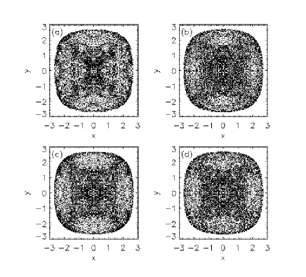
FIG. 8.: (a) A collection of 20000 orbits sampling a near-invariant distribution with energy $E=6.0$ in the two-dimensional dihedral potential with $a=1$ at time $t=36.0$. (b) The same orbits sampled at a much later time $t=720$. Both ensembles were generated from a localised collection of initial conditions corresponding to ‘wildly chaotic’ orbits. (c) The same orbits, now evolved in white noise with ${\Theta}=6.0$ and ${\eta}=10^{-6}$, again sampled at $t=36.0$. (d). White noise with ${\Theta}=6.0$ and ${\eta}=10^{-5}$, sampled at $t=36.0$.

FIG. 9.: The quantity $\ln|{\langle}x{\rangle}|$ computed for an initially localised ensemble of regular orbits with $E=2.0$ evolved in the potential (2.2) with $a=b=c=1$. (a) No noise. (b) ${\eta}=10^{-7}$. (c) ${\eta}=10^{-6}$. (d) ${\eta}=10^{-5}$.

FIG. 10.: The dispersion ${\sigma}_{x}$ computed for initially localised ensembles of evolved in the two-dimensional dihedral potential with $a=1$ in the presence of friction and white noise with ${\Theta}=E$ and (from bottom to top) variable ${\eta}=0$, $10^{-7}$, $10^{-5}$, and $10^{-4}$. The three upper curves were shifted upwards by amounts $2$, $4$, and $6$. (a) A ‘wildly chaotic’ ensemble with $E=2.0$. (b) A ‘sticky’ ensemble with $E=4.0$.

FIG. 11.: The quantity $Df(x,y)$ computed for the ‘wildly chaotic’ (a) and ‘sticky’ (b) ensembles used to generate the preceding Figure, again staggered by translations of $2$, $4$, and $6$.

FIG. 12.: ${\Lambda}$, the rate at which $f(x,y)$ approaches a near-invariant distribution, computed as a function of ${\eta}$ for the ‘wildly chaotic’ ensemble used to generate Fig. 11. The dashed line corresponds to the zero noise limit.

FIG. 13.: (a) The dispersion ${\sigma}_{x}$ computed for the ensemble used to generate Figs. 11 b and 12 b, now integrated in the presence of Ornstein-Uhlenbeck noise with ${\Theta}=4.0$, ${\eta}=10^{-5}$ and (from top to bottom) ${\alpha}=100.0$, ${\alpha}=10.0$, ${\alpha}=3.33$, ${\alpha}=1.0$, ${\alpha}=0.33$, and ${\alpha}=0.1$, corresponding to autocorrelation times $t_{c}=0.01$, $0.1$, $0.33$, $1.0$, $3.33$, and $10.0$. (b) The quantity $\ln|{\langle}x{\rangle}|$ computed for the same ensembles.

FIG. 14.: The analogue of Fig. 13, now computed for orbits in the presence of coloured noise characterised by the more complex autocorrelation function (2.12).

FIG. 15.: (a) ${\Lambda}$, the rate at which $f(x,y)$ approaches a near-invariant distribution, computed as a function of $t_{c}$ for a ‘wildly chaotic’ ensemble with $E=2.0$ evolved in the presence of Ornstein-Uhlenbeck noise with ${\Theta}=1.0$ and ${\eta}=10^{-5}$. The lower dashed line corresponds to evolution in the absence of noise. The upper line corresponds to the $t_{c}=0$ white noise limit. (b) The analogue of (a), now computed for noise with the autocorrelation function (2.12).

FIG. 16.: (a) The maximum value of ${\sigma}_{E}$ for the ensemble used to generate Figs. 10 and 11b, now evolved for a time $t=256$ in the presence of periodic driving of the form given by eq. (2.7) with fixed amplitude $A=10^{-2}$ but different frequencies ${\omega}$, expressed in units of the original energy $E_{0}=4.0$. (b) The same for driving of the form given by eq. (2.5), again with $A=10^{{}_{2}}$. (c) The composite power spectra, $|x({\omega})|$ (solid curve) and $|y({\omega})|$ (dashed) computed for the unperturbed ensemble.

FIG. 17.: (a) The dispersion ${\sigma}_{x}$ computed for an ensemble evolved in the two-dimensional dihedral potential with $a=1$ in the absence of all perturbations (lower curve) and in the presence of periodic driving of the form (2.7) with $A=10^{-1.5}$ and (from bottom to top) ${\omega}=0.1$, ${\omega}=1.0$, ${\omega}=3.0$, ${\omega}=10.0$, and ${\omega}=30.0$. The upper curves were shifted upwards by amounts $4$, $8$, $12$, $16$, and $20$. (b) The quantity $\ln|{\langle}x{\rangle}|$ for the same ensembles, the upper curves again staggered.