Abstract

The last years have been an exciting period for the field of the Cosmic Microwave Background (CMB) research. With recent CMB balloon-borne and ground-based experiments we are entering a new era of ’precision’ cosmology that enables us to use the CMB anisotropy measurements to constrain the cosmological parameters and test new theoretical scenarios.

CMB and Cosmological Parameters: Current Status and Prospects.

¹ Denys Wilkinson Building, University of Oxford, Keble Road, Oxford, OX1 3RH, UK.

0.1 Introduction

The last years have been an exciting period for the field of the Cosmic Microwave Background (CMB) research. With recent CMB balloon-borne and ground-based experiments we are entering a new era of ’precision’ cosmology that enables us to use the CMB anisotropy measurements to constrain the cosmological parameters and the underlying theoretical models.

Coeherent oscillations in the Cosmic Microwave Background anisotropies angular power spectrum have been predicted since long time from simple assumptions about scale invariance and linear perturbation theory (see e.g., [119], [132], [150], [143], [21]). The physics of these oscillations and their dependence on the various cosmological parameters has been described in great detail in many reviews ([81], [80], [149], [19], [45], [111]). Basically, on sub-horizon scales, prior to recombination, photons and baryons form a tightly coupled fluid that performs acoustic oscillations driven by the gravitational potential. These acoustic oscillations define a structure of peaks in the CMB angular power spectrum that can be measured today.

With the TOCO$-97/98$ ([138],[112]) and Boomerang-$97$ ([104]) experiments a firm detection of a first peak on about degree scales has been obtained. In the framework of adiabatic Cold Dark Matter (CDM) models, the position, amplitude and width of this peak provide strong supporting evidence for the inflationary predictions of a low curvature (flat) universe and a scale-invariant primordial spectrum ([51], [109], [134]).

The new experimental data from BOOMERANG LDB ([116]), DASI ([69]) and MAXIMA ([95]) have provided further evidence for the presence of the first peak and refined the data at larger multipole. The combined data clearly suggest the presence of a second and third peak in the spectrum, confirming the model prediction of acoustic oscillations in the primeval plasma and sheding new light on various cosmological and inflationary parameters ([17], [145], [123]).

0.2 The Current Observational Status.

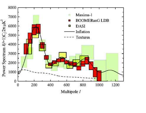
Figure 1: BOOMERanG, DASI and MAXIMA data togheter with an inflationary model and a global textures model.

On April 30th 2001, at the same time, $3$ different teams, BOOMERanG [116], DASI [69] and MAXIMA [95] reported a detection of multiple features in the CMB angular power spectrum.

The BOOMERanG experiment. BOOMERanG is a scanning balloon experiment aimed at producing accurate and high signal/noise maps of the CMB sky and constraining the power spectrum in the $50<\ell<1000$ range. The BOOMERanG experiment has been described in [122] and [15]. All the relevant informations about the collaboration can be found in the ’official’ websites: http://oberon.roma1.infn.it/boom and http://www.physics.ucsb.edu/b̃oomerang/.

The BOOMERanG group carried out a long duration flight (December 1998/ January 1999) called the Antarctica or LDB flight. Before this, there was a ’test flight’ on North America from which the first power spectrum results were released ([104], [109], [122]). From the test flight a $\sim 4000$ $16^{\prime}$ pixel map at $150GHz$ produced a firm detection of a first peak in the CMB angular power spectrum.

For the antarctica flight, coverage of $4$ frequencies with $16$ bolometers in total were available. BOOMERanG LDB measured $8$ pixels in the sky simultaneously . Four pixels feature multiband photometers ($150$, $240$ and $410$ GHz), two pixels have single-mode, diffraction limited detectors at $150$ GHz and two pixels have single-mode, diffraction limited detectors at $90$ GHz. The NEP of these detectors is below $200\mu K_{CMB}\sqrt{s}$ at $90$, $150$ and $240$ GHz and the angular resolution ranges from $12$ to $18$ arcminFWHM.

The istrument was flown aboard a stratospheric balloon at $38Km$ of altitude to avoid the bulk of atmospheric emission and noise. During a long duration balloon flight of $\sim 11$ days carried out by NASA-NSBF around Antarctica in $1999$, BOOMERanG mapped $\sim 1800$ square degrees in a region of the sky with minimal contamination from the galaxy.

The most recent analysis of the BOOMERanG data has been presented in [116]. The observations taken from $4$ detectors at $150$ GHz in a dust-free ellipsoid central region of the map ($1.8\%$ of the sky) have been analyzed using the methods of ([22], [77], [124]). The gain calibration are obtained from observations of the CMB dipole.

The CMB angular power spectrum, estimated in $19$ bands centered between $\ell=50$ to $\ell=1000$ is shown in Figure 1. The error bars on the $y$ axis are correlated at about $\sim 10\%$. A first peak is clearly evident at $\ell\sim 200$ and $2$ subsequent peaks can be see in the figure. Not shown in the figure is an additional $10\%$ calibration error (in $\Delta T$) and the uncertainty in the beam size ($12.9^{\prime}\pm 1.4^{\prime}$).

Calibration error does not affect the shape of the power spectrum, producing only an overall shift in amplitude.

On the contrary, since the beam resolution affects the $C_{\ell}$ spectrum, a small uncertainty $\Delta\sigma^{2}_{beam}=\sigma^{2}_{beam}-(\sigma_{beam}^{\prime})^{2}$ in the telescope beam produce a correlated $\ell$-dependent ’calibration error’ of $\sim(1+\ell^{2}\Delta\sigma^{2}_{beam})C_{\ell}$ ([26])

The beam uncertainty can change the relative amplitude of the peaks, but cannot introduce features in the spectrum.

The DASI experiment. The DASI experiment is a ground based compact interferometer constructed specifically for observations of the CMB. A description of the instrument can be found in [69] and [96]. and all the relevant information about the team can be obtained from the DASI website:http://astro.uchicago.edu/dasi/.

The specific advantage of interferometers is in reducing the effects of atmospheric emission [92]. DASI is composed of $13$ element interferometers with correlator operating from $26$ to $36$ GHz. The baseline of DASI cover angular scales from $15^{\prime}$ to $1.4^{o}$.

Interferometry is a technique that differs in many fundamental ways from those used by BOOMERanG and other map-making CMB experiments. Interferometers directly sample the Fourier transform of the sky brightness distribution and the CMB power spectrum can be computed without going through the map making process. In this sense, the DASI result provides a real independent observation of the CMB angular spectrum.

The most recent analysis of the DASI data has been presented in [69]. The observations have been taken over $97$ days from the South-Pole during the austral summer at frequencies between $26$ and $36$ GHz. The calibration was obtained using bright astronomical sources.

The CMB angular power spectrum estimated in $9$ bands between $\ell=100$ to $\ell=900$ is also shown in Figure 1. There is a $\sim 20\%$ correlation between the data points. Not shown in the figure is an $\sim 8\%$ calibration error, while the beam error is negligible. The DASI team found no evidence for foregrounds other than point sources (which are the dominant foregrounds at those frequencies (see e.g. [135], [136])). Nearly $30$ point sources have been detected in the DASI data while a statistical correction has been made for residual point sources that were too faint to be detected.

The MAXIMA experiment. MAXIMA-I is another balloon experiment, similar in many aspects to BOOMERang but not long-duration. A description of the instrument can be found in [95] and all the relevant informations about the team can be obtained from the MAXIMA website: http://cosmology.berkeley.edu/group/cmb/. In the latest analysis ([95]) the data from $3$, $150$, GHz very sensitive bolometers has been analyzed in order to produce a $3^{\prime}$ pixelized map of about $10$ by $10$ degrees. The previous analysis of about the same data based on a $5^{\prime}$ pixelization ([70]) has therefore been extended to $\ell=1235$. The map-making method used by the MAXIMA team is extensively discussed in [131]. The data are calibrated using the CMB dipole.

The MAXIMA-I datapoints are also shown in Figure 1. The error bars are correlated at level of $\sim 10\%$. The $\sim 4\%$ calibration error is not plotted in the figure. The beam/pointing errors are of order of $\sim 10\%$ at $\ell=1000$ (see [95]).

Features in the CMB power spectrum.

Before going on to parameter extraction, it is important to try to quantify how well the present data provide evidence for multiple and coherent oscillations. Fits to the CMB data with phenomenological functions have been already extensively used in the past (see e.g. [126], [128], [90]). More recently, similar analyses have been carried out, using parabolas ([17], [49]) or more elaborate oscillating functions with a well defined frequency and phase ([43]).

Since the first peak is evident, the statistical significance of the secondary oscillations is now of greater interest. In [17] the BOOMERanG data bins centered at $450<\ell<1000$ were analyzed. Using a Bayesian approach, a linear fit $C_{\ell}^{T}=C_{A}+C_{B}\ell$ is rejected at near $2\sigma$ confidence level. Also in [17], using a parabolic fit to the data, interleaved peaks and dips were found at $\ell=$ $215\pm 11$, $431\pm 10$, $522\pm 27$, $736\pm 21$ and $837\pm 15$ with amplitudes of the features $5760^{+344}_{-324}$, $1890^{+196}_{-178}$, $2290^{+330}_{-290}$, $1640^{+500}_{-380}$, and $2210^{+900}_{-640}$ $\mu K^{2}$, correspondingly. The reported significance of the detection is $1.7\,\sigma$ for the second peak and dip, and $2.2\,\sigma$ for the third peak.

The evidence for oscillations in the MAXIMA data has been carefully studied in [130]. While there is no evidence for a second peak, the power spectrum shows excess power at $\ell\sim 860$ over the average level of power at $411\leq\ell\leq 785$ on the $95\%$ confidence level. Such a feature is consistent with the presence of a third acoustic peak.

In [49] the BOOMERanG, DASI and MAXIMA data were included in a similar analysis. Both DASI and MAXIMA confirmed the main features of the Boomerang CMB power spectrum: a dominant first acoustic peak at $\ell\sim 200$, DASI shows a second peak at $\ell\sim 540$ and MAXIMA-I exhibits mainly a ’third peak’ at $\ell\sim 840$.

Finally and more recently, in [43] a different analysis was made, based on a function that smoothly interpolates between a spectrum with no oscillations and one with oscillations. Again, within the context of this different phenomenological model, a $2\sigma$ presence for secondary oscillations was found.

0.3 Consequences for Cosmology

In principle, the CDM scenario of structure formation based on adiabatic primordial fluctuations can depend on more than $11$ parameters.

However for a first analysis, it is useful to restrict ourselves to just $5$ parameters: the tilt of primordial spectrum of perturbations $n_{S}$, the optical depth of the universe $\tau_{c}$, the density in baryons and dark matter $\omega_{b}=\Omega_{b}h^{2}$ and $\omega_{dm}=\Omega_{dm}h^{2}$ and the shift parameter ${\cal R}$ which is related to the geometry of the universe through (see [53], [107]):

$${\cal R}=2\sqrt{|\Omega_{k}|/\Omega_{m}}/\chi(y)$$ (1)

where $\Omega_{m}=\Omega_{b}+\Omega_{dm}$, $\Omega_{k}=1-\Omega_{m}-\Omega_{\Lambda}$, the function $\chi(y)$ is $y$, $\sin(y)$ or $\sinh(y)$ for flat, closed and open universes respectively and

$$y=\sqrt{|\Omega_{k}|}\int_{0}^{z_{dec}}{[\Omega_{m}(1+z)^{3}+\Omega_{k}(1+z)^{2}+\Omega_{\Lambda}]^{-1/2}dz}.$$ (2)

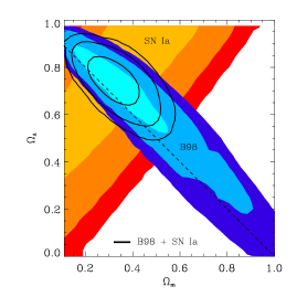
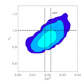
Figure 2: Confidence contours in the $\Omega_{M}-\Omega_{\Lambda}$ and $\Omega_{b}h^{2}-n_{S}$ planes. Picture taken from [17].

The restriction of the analysis to only $5$ parameters is justified since a reasonable fit to the data can be obtained with no additional parameters.

In Fig. 2 we plot the likelihood contours on the $\Omega_{M}-\Omega_{\Lambda}$ and $\Omega_{b}h^{2}-n_{S}$ planes from the BOOMERanG experiment as reported in [17]. Since the quantity ${\cal R}$ depends on $\Omega_{\Lambda}$ and $\Omega_{M}$ the CMB constraints on this parameter can be plotted on this plane. As we can see from the top panel in the figure the data strongly suggest a flat universe (i.e. $\Omega=\Omega_{M}+\Omega_{\Lambda}=1$). From the latest BOOMERanG data one obtains $\Omega=1.02\pm 0.06$ ([116]).

The inclusion of complementary datasets in the analysis breaks the angular diameter distance degeneracy in $\cal R$ and provides evidence for a cosmological constant at high significance. Adding the Hubble Space Telescope constraint on the Hubble constant $h=0.72\pm 0.08$ ([62], information from galaxy clustering and from luminosity distance of type Ia supernovae gives ([116]) $\Omega_{\Lambda}=0.62_{-0.18}^{+0.10}$, $\Omega_{\Lambda}=0.55_{-0.09}^{+0.09}$ and $\Omega_{\Lambda}=0.73_{-0.07}^{+0.10}$ respectively.

Also interesting is the plot of the likelihood contours in the $\Omega_{b}h^{2}-n_{S}$ plane (Fig.2 bottom panel). As we can see, the present BOOMERanG data is in beautiful agreement with both a nearly scale invariant spectrum of primordial fluctuations, as predicted by inflation, and the value for the baryon density $\omega_{b}=0.020\pm 0.002$ predicted by Standard Big Bang Nucleosynthesis (see e.g. [28]).

An increase in the optical depth $\tau_{c}$ after recombination by reionization (see e.g. [68] for a review) or by some more exotic mechanism damps the amplitude of the CMB peaks. Even if degeneracies with other parameters such as $n_{S}$ are present (see e.g. [14]) the BOOMERanG data provides the upper bound $\tau_{c}<0.3$.

The amount of non-baryonic dark matter is also constrained by the CMB data with $\Omega_{dm}h^{2}=0.13\pm 0.04$ at $68\%$ c.l. ([116]). The presence of power around the third peak is crucial in this sense, since it cannot be easily accommodated in models based on just baryonic matter (see e.g. [108], [65], [106] and references therein).

Furthermore, under the assumption of flatness, we can derive important constraints on the age of the universe $t_{0}$ given by:

$$t_{0}=9.8Gy\int_{0}^{1}{{ada\over{[\omega_{m}a+\omega_{\Lambda}a^{4}]^{1/2}}}}$$ (3)

In [59] the BOOMERanG constraint on age has been compared with other independent results obtained from stellar populations in bright ellipticals, ²³⁸U age-measurement of an old halo star in our galaxy ([31]) and age the of the oldest halo globular cluster in the sample of Salaris & Weiss ([127]). All four methods give completely consistent results, and enable us to set rigorous bounds on the maximum and minimum ages that are allowed for the universe, $t_{0}=14\pm 1$ GYrs ([59], [116],[89]).

The results from the DASI experiment have been extensively reported in [123] and are perfectly consistent with the BOOMERanG results. Pryke et al. report $\Omega=1.04\pm 0.06$, $n_{s}=1.01^{0.08}_{0.06}$, $\Omega_{b}h^{2}=0.022^{0.004}_{0.003}$ and $\Omega_{dm}h^{2}=0.14\pm 0.04$.

The MAXIMA team reported similar compatible constraints in [130]: $\Omega=0.9{+0.18\atop-0.16}$ and $\Omega_{b}h^{2}=0.033{\pm 0.13}$ at $2\sigma$ c.l.. However the MAXIMA data is not good enough to put strong constrains on the spectral index $n_{S}$ and the optical depth $\tau_{c}$ because of the degeneracy between the $2$ parameters.

0.4 Open Questions.

Even if the present CMB observations can be fitted with just $5$ parameters it is interesting to extend the analysis to other parameters allowed by the theory. Here I will just summarize a few of them and discuss how well we can constrain them and what the effects on the results obtained in the previous section would be.

Gravity Waves. The metric perturbations created during inflation belong to two types: scalar perturbations, which couple to the stress-energy of matter in the universe and form the “seeds” for structure formation and tensor perturbations, also known as gravitational wave perturbations. Both scalar and tensor perturbations contribute to CMB anisotropy. In the recent CMB analysis by the BOOMERanG and DASI collaborations, the tensor modes have been neglected, even though a sizable background of gravity waves is expected in most of the inflationary scenarios. Furthermore, in the simplest models, a detection of the GW background can provide information on the second derivative of the inflaton potential and shed light on the physics at $\sim 10^{16}Gev$ (see e.g. [78]).

The shape of the $C^{T}_{\ell}$ spectrum from tensor modes is drastically different from the one expected from scalar fluctuations, affecting only large angular scales (see e.g. [35]). The effect of including tensor modes is similar to just a rescaling of the degree-scale $COBE$ normalization and/or a removal of the corresponding data points from the analysis.

This further increases the degeneracies among cosmological parameters, affecting mainly the estimates of the baryon and cold dark matter densities and the scalar spectral index $n_{S}$ ([110],[85], [145], [52]).

The amplitude of the GW background is therefore weakly constrained by the CMB data alone, however, when information from BBN, local cluster abundance and galaxy clustering are included, an upper limit of about $r=C_{2}^{T}/C_{2}^{S}<0.5$ is obtained.

Scale-dependence of the spectral index. The possibility of a scale dependence of the scalar spectral index, $n_{S}(k)$, has been considered in various works (see e.g. [91], [32], [100], [38]). Even though this dependence is considered to have small effects on CMB scales in most of the slow-roll inflationary models, it is worthwhile to see if any useful constraint can be obtained. Allowing the power spectrum to bend erases the ability of the CMB data to measure the tensor to scalar perturbation ratio and enlarge the uncertainties on many cosmological parameters.

Recently, Covi and Lyth ([34]) investigated the two-parameter scale-dependent spectral index predicted by running-mass inflation models, and found that present CMB data allow for a significant scale-dependence of $n_{S}$. In Hannestad et al. ([73], [74]) the case of a running spectral index has been studied, expanding the power spectrum $P(k)$ to second order in $ln(k)$. Again, their result indicates that a bend in the spectrum is consistent with the CMB data.

Furthermore, phase transitions associated with spontaneous symmetry breaking during the inflationary era could result in the breaking of the scale-invariance of the primordial density perturbation. In [9], [66] and [144] the possibility of having step or bump-like features in the spectrum has also been considered.

While much of this work was motivated by the tension between the initial release of the data and the baryonic abundance value from BBN, a sizable feature in the spectrum is still compatible with the latest CMB data ([54]).

Quintessence. The discovery that the universe’s evolution may be dominated by an effective cosmological constant [63] is one of the most remarkable cosmological findings of recent years. One candidate that could possibly explain the observations is a dynamical scalar “quintessence” field. One of the strongest aspects of quintessence theories is that they go some way towards explaining the fine-tuning problem, that is why the energy density producing the acceleration is $\sim 10^{-120}M_{pl}^{4}$. A vast range of “tracker” (see for example [152, 25]) and “scaling” (for example [148], [58]) quintessence models exist which approach attractor solutions, giving the required energy density, independent of initial conditions. The common characteristic of quintessence models is that their equations of state, $w_{Q}=p/\rho$, vary with time while a cosmological constant remains fixed at $w_{Q=\Lambda}=-1$ (see e.g. [18]). Observationally distinguishing a time variation in the equation of state or finding $w_{Q}$ different from $-1$ will therefore be a success for the quintessential scenario. Quintessence can also affect the CMB by acting as an additional energy component with a characteristic viscosity. However any early-universe imprint of quintessence is strongly constrained by Big Bang Nucleosynthesis with $\Omega_{Q}(MeV)<0.045$ at $2\sigma$ for temperatures near $T\sim 1Mev$ ([11], [151]).

In [12] we have combined the latest observations of the CMB anisotropies and the information from Large Scale Structure (LSS) with the luminosity distance of high redshift supernovae (SN-Ia) to put constraints on the dark energy equation of state parameterized by a redshift independent quintessence-field pressure-to-density ratio $w_{Q}$.

The importance of combining different data sets in order to obtain reliable constraints on $w_{Q}$ has been stressed by many authors (see e.g. [121], [79],[147]), since each dataset suffers from degeneracies between the various cosmological parameters and $w_{Q}$ . Even if one restricts consideration to flat universes and to a value of $w_{Q}$ constant in time then the SN-Ia luminosity distance and position of the first CMB peak are highly degenerate in $w_{Q}$ and $\Omega_{Q}$, the energy density in quintessence.

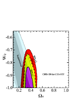
Figure 3: The likelihood contours in the ($\Omega_{M}$, $w_{Q}$) plane, with the remaining parameters taking their best-fitting values for the joint CMB+SN-Ia+LSS analysis described in the text. The contours correspond to 0.32, 0.05 and 0.01 of the peak value of the likelihood, which are the 68%, 95% and 99% confidence levels respectively. Picture taken from [12].

In Figure 3 we plot the likelihood contours in the ($\Omega_{M}$, $w_{Q}$) plane for the joint analyses of CMB+SN-Ia+HST+LSS of [12] together with the contours from the SN-Ia dataset only. As we can see, the combination of the datasets breaks the luminosity distance degeneracy and suggests the presence of dark energy with high significance. Furthermore, the new CMB results provided by Boomerang and DASI improve the constraints from previous and similar analysis (see e.g., [121],[20]), with $w_{Q}<-0.85$ at $68\%$ c.l.. Our final result is then perfectly in agreement with the $w_{Q}=-1$ cosmological constant case and gives no support to a quintessential field scenario with $w_{Q}>-1$.

Big Bang Nucleosynthesis and Neutrinos. As we saw in the previous section, the SBBN $95\%$ CL region, corresponding to $\Omega_{b}h^{2}=0.020{\pm}0.002$ ($95\%$ c.l.), has a large overlap with the analogous CMBR contour. This fact, if it will be confirmed by future experiments on CMB anisotropies, can be seen as one of the greatest success, up to now, of the standard hot big bang model.

SBBN is well known to provide strong bounds on the number of relativistic species $N_{\nu}$. On the other hand, Degenerate BBN (DBBN), first analyzed in Ref. [41, 61, 13, 83], gives very weak constraint on the effective number of massless neutrinos, since an increase in $N_{\nu}$ can be compensated by a change in both the chemical potential of the electron neutrino, $\mu_{\nu_{e}}=\xi_{e}T$, and $\Omega_{b}h^{2}$. Practically, SBBN relies on the theoretical assumption that background neutrinos have negligible chemical potential, just like their charged lepton partners. Even though this hypothesis is perfectly justified by Occam razor, models have been proposed in the literature [36, 1, 39, 40, 30, 102, 105, 60], where large neutrino chemical potentials can be generated. It is therefore an interesting issue for cosmology, as well as for our understanding of fundamental interactions, to try to constrain the neutrino–antineutrino asymmetry with the cosmological observables. It is well known that degenerate BBN gives severe constraints on the electron neutrino chemical potential, $-0.06\leq\xi_{e}\leq 1.1$, and weaker bounds on the chemical potentials of both the $\mu$ and $\tau$ neutrino, $|\xi_{\mu,\tau}|\leq 5.6\div 6.9$ [83], since electron neutrinos are directly involved in neutron to proton conversion processes which eventually fix the total amount of ${}^{4}He$ produced in nucleosynthesis, while $\xi_{\mu,\tau}$ only enters via their contribution to the expansion rate of the universe.

Combining the DBBN scenario with the bound on baryonic and radiation densities allowed by CMBR data, it is possible to obtain strong constraints on the parameters of the model. Such an analysis was previously performed in ([57], [98], [71], [117]) using the first data release of BOOMERanG and MAXIMA ([16], [70]). We recall that the neutrino chemical potentials contribute to the total neutrino effective degrees of freedom $N_{\nu}$ as

$$N_{{\nu}}=3+\Sigma_{\alpha}\left[\frac{30}{7}\left(\frac{\xi_{\alpha}}{\pi}\right)^{2}+\frac{15}{7}\left(\frac{\xi_{\alpha}}{\pi}\right)^{4}\right]\,.$$ (4)

Notice that in order to get a bound on $\xi_{\alpha}$ we have here assumed that all relativistic degrees of freedom, other than photons, are given by three (possibly) degenerate active neutrinos.

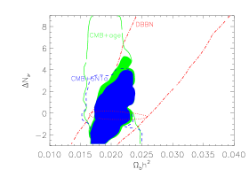
Figure 4: The $95\%$ CL contours for degenerate BBN (dot-dashed (green) line), new CMB results with just the age prior, $t>11$gyr (full (red) line), and with just the SN1a prior (dashed (blue) line). The combined analysis corresponds to the filled regions. Marginalization leads to the bound $\Omega_{b}h^{2}=0.020{\pm}0.0035$ and $N_{\nu}<7$, both at $95\%$, for DBBN+CMB+SN. The dotted (green) line is the $95\%$ CL allowed by SBBN. Picture taken from [76].

Figure 4 summarizes the main results with the new CMB data, reported in [76] for the DBBN scenario. We plot the $95\%$ CL contours allowed by DBBN (dot-dashed (green) line), together with the analogous $95\%$ CL region coming from the CMB data analysis, with only weak age prior, $t_{0}>11$gyr (full (red) line).

Finally, the solid contour (light, red) is the $95\%$ CL region of the joint product distribution ${\cal L}\equiv{\cal L}_{DBBN}$${\cdot}{\cal L}_{CMB}$. The main new feature, with respect to the results of Ref. [57] is that the resolution of the third peak shifts the CMB likelihood contour towards smaller values for $\Omega_{b}h^{2}$, so when combined with DBBN results, it singles out smaller values for $N_{\nu}$. In fact from our analysis we get the bound $N_{\nu}\leq 8$, at $95\%$ CL, which translates into the new bounds $-0.01\leq\xi_{e}\leq 0.25$, and $|\xi_{\mu,\tau}|\leq 2.9$, sensibly more stringent than what can be found from DBBN alone.

A similar analysis can also be performed combining CMBR and DBBN data with the Supernova Ia data [63], which strongly reduces the degeneracy between $\Omega_{m}$ and $\Omega_{\Lambda}$. At $95\%$ C.L. we find $\Delta N_{\nu}<7$, corresponding to $-0.01\leq\xi_{e}\leq 0.22$ and $|\xi_{\mu,\tau}|\leq 2.6$.

Compatible results have been obtained in similar analyses ([86],[72]).

Some caution is naturally necessary when comparing the effective number of neutrino degrees of freedom from BBN and CMB, since they may be related to different physics. In fact the energy density in relativistic species may change from the time of BBN ($T\sim MeV$) to the time of last rescattering ($T\sim eV$).

Varying $\alpha$. There are quite a large number of experimental constraints on the value of fine structure constant $\alpha$. These measurements cover a wide range of timescales (see [141] for a review of this subject), starting from present-day laboratories ($z\sim 0$), geophysical tests ($z<<1$), and quasars ($z\sim 1\div 3$), through the CMB ($z\sim 10^{3}$) and BBN ($z\sim 10^{10}$) bounds.

The recent analysis of [113] of fine splitting of quasar doublet absorption lines gives a $4\sigma$ evidence for a time variation of $\alpha$, $\Delta\alpha/\alpha=(-0.72{\pm}0.18)10^{-5}$, for the redshift range $z\sim 0.5-3.5$. This positive result was obtained using a many-multiplet method, which, it is claimed, achieves an order of magnitude greater precision than the alkali doublet method. Some of the initial ambiguities of the method have been tackled by the authors with an improved technique, in which a range of ions is considered, with varying dependence on $\alpha$, which helps reduce possible problems such as varying isotope ratios, calibration errors and possible Doppler shifts between different populations of ions [114, 29, 146, 115].

The present analysis of the $\alpha$-dependence relevant cosmological observables like the anisotropy of CMB, Large Scale Structure and the light element primordial abundances does not support evidence for variations of the fine-structure constant (see [5], [103] and references therein).

Isocurvature modes. Another key assumption is that the primordial fluctuations were adiabatic. Adiabaticity is not a necessary consequence of inflation though and many inflationary models have been constructed where isocurvature perturbations would have generically been concomitantly produced (see e.g. [94], [64], [10]).

In a phenomenological approach one should consider the most general primordial perturbation, introduced by [27], and described by a $5X5$ symmetric matrix-valued generalization of the power spectrum. As showed by [27], the inclusion of isocurvature perturbations with auto and cross-correlations modes has dramatic effects on standard parameter estimation with uncertainties becoming of order one.

Even assuming priors such as flatness, the inclusion of isocurvature modes significantly enlarges our constraints on the baryon density [139] and the scalar spectral index [4]. Pure isocurvature perturbations are highly excluded by present CMB data ([56]).

As we saw in the first section, it is also possible to have active and decoherent perturbations such as those produced by an inhomogeneously distributed form of matter like topological defects. Models based on global defects like cosmic strings and textures are excluded at high significance by the present data (see e.g. [47]). However a mixture of adiabatic$+$defects is still compatible with the observations ([23], [47]). In principle, toy models based on active perturbations can be constructed [140] that can mimic inflation and retain a good agreement with observations [48].

Secondary anisotropies. Secondary anisotropies can be generated due to photon interactions with the matter potential wells (for example in the Rees-Sciama effect [125] and lensing [129]). The other secondary anisotropies are induced by the interaction of CMB photons with free electrons such as in the Sunyaev-Zel’dovich (SZ) effect [133], the Ostriker-Vishniac (OV) effect ([118], [142]), and because of early inhomogeneous reionisation (IHR) ([2],[67],[88]).

Figure 5: Primary and Secondary CMB anisotropies. The $95\%$ confidence levels for the primary anisotropies are plotted together with the extreme predictions allowed (within $2\sigma$) by the present parameter estimations. The SZ effect at 150 GHz is displayed in solid lines, the IHR and OV contributions are plotted with dotted and dashed lines, respectively.

Recent works (se e.g. [33], [3] and references therein) have quantified the contribution of the secondary scattering effects that are likely the dominant contributions at small scales. In Figure 5, taken from [3], predictions for the level of primary and secondary anisotropies are plotted, given the current status of observations. As we can see, in some extreme cosmological model, the secondary signal can be high enough to match the power of the CMB primary anisotropies after the third peak. Future small-scale CMB data such as that expected from CBI [101], will definitely be helpful in scrutinising this results. The measurements of the CMB anisotropies after the third peak will therefore not only constrain the cosmological model through parameter estimation, but will also unable us to probe, via the secondary anisotropies (e.g. SZ), the formation and evolution of structures.

0.5 Conclusions

The recent CMB data represent a beautiful success for the standard cosmological model. The acoustic oscillations in the CMB angular power spectrum, a major prediction of the model, have now been detected at $\sim 5\sigma$ C.L. for the first peak and $\sim 2\sigma$ C.L. for the second and third peak. Furthermore, when constraints on cosmological parameters are derived under the assumption of adiabatic primordial perturbations their values are in agreement with the predictions of the theory and/or with independent observations.

As we saw in the previous section modifications as isocurvature modes or topological defects, are still compatible with current CMB observations, but are not necessary and can be reasonably constrained when complementary datasets are included.

Since the inflationary scenario is in agreement with the data and all the most relevant parameters are starting to be constrained within a few percent accuracy, the CMB is becoming a wonderful laboratory for investigating the possibilities of new physics. With the promise of large data sets from Map, Planck and SNAP satellites, opportunities may be open, for example, to constrain dark energy models, variations in fundamental constants and neutrino physics.

Acknowledgements

I wish to thank the organizers of the conference: L. Celnikier and J. Tran ThanhVan. Many thanks also to Nabila Aghanim, Rachel Bean, P.G. de Castro, Ruth Durrer, Steen Hansen, Pedro Ferreira, Will Kinney, Gianpiero Mangano, Carlos Martins, Gennaro Miele, Ofelia Pisanti, Antonio Riotto, Graca Rocha, Joe Silk, and Roberto Trotta for comments, discussions and help.

Bibliography

- [1] I. Affleck and M. Dine, Nucl. Phys. B249 (1985) 361.
- [2] Aghanim, N., Désert, F. X., Puget, J. L. & Gispert, R. 1996, A&A, 311, 1.
- [3] N. Aghanim, P. G. Castro, A. Melchiorri and J. Silk, arXiv:astro-ph/0203112.
- [4] L. Amendola, C. Gordon, D. Wands and M. Sasaki, arXiv:astro-ph/0107089.
- [5] P. P. Avelino et al., Phys. Rev. D 64, 103505 (2001) [arXiv:astro-ph/0102144].
- [6] A. Balbi et al., Astrophys. J. 545 (2000) L1 [Erratum-ibid. 558 (2000) L145] [arXiv:astro-ph/0005124].
- [7] J.M Bardeen, Phys. Rev. D22 1882–1905, 1980.
- [8] V. Barger, C. Kao, hep-ph/0106189
- [9] J. Barriga, E. Gaztanaga, M. G. Santos and S. Sarkar, Mon. Not. Roy. Astron. Soc. 324 (2001) 977 [arXiv:astro-ph/0011398].
- [10] N. Bartolo, S. Matarrese and A. Riotto, Phys. Rev. D 64 (2001) 123504 [arXiv:astro-ph/0107502].
- [11] R. Bean, S. H. Hansen and A. Melchiorri, Phys. Rev. D 64 (2001) 103508 [arXiv:astro-ph/0104162].
- [12] R. Bean and A. Melchiorri, arXiv:astro-ph/0110472, Phys. Rev. D Rapid Communication, in press.
- [13] G. Beaudet and P. Goret, Astron. & Astrophys. 49 (1976) 415.
- [14] P. de Bernardis, A. Balbi, G. De Gasperis, A. Melchiorri and N. Vittorio, arXiv:astro-ph/9609154.
- [15] P. de Bernardis et al. [Boomerang Collaboration] astro-ph/9911461.
- [16] P. de Bernardis et al. [Boomerang Collaboration], Nature 404, 955 (2000) [arXiv:astro-ph/0004404].
- [17] P. de Bernardis et al., [Boomerang Collaboration], arXiv:astro-ph/0105296.
- [18] S. A. Bludman and M. Roos, arXiv:astro-ph/0109551.
- [19] J. R. Bond, Class. Quant. Grav. 15 (1998) 2573.
- [20] J. R. Bond et al. [The MaxiBoom Collaboration], astro-ph/0011379.
- [21] J. R. Bond and G. Efstathiou, Astrophys. J. 285 (1984) L45.
- [22] J. Borrill, proceedings of ‘3K Cosmology Euroconference’, Roma, ed F. Melchiorri, astro-ph/9903204.
- [23] F. R. Bouchet, P. Peter, A. Riazuelo and M. Sakellariadou, Phys. Rev. D 65 (2002) 021301 [arXiv:astro-ph/0005022].
- [24] R. Bowen et al., arXiv:astro-ph/0110636.
- [25] P. Brax, J. Martin & A. Riazuelo, Phys. Rev. D.,62 103505 (2000).
- [26] S. L. Bridle, R. Crittenden, A. Melchiorri, M. P. Hobson, R. Kneissl and A. N. Lasenby, arXiv:astro-ph/0112114.
- [27] M. Bucher, K. Moodley and N. Turok, Phys. Rev. D 62 (2000) 083508 [arXiv:astro-ph/9904231].
- [28] S. Burles, K. M. Nollett and M. S. Turner, Astrophys. J. 552, L1 (2001) [arXiv:astro-ph/0010171].
- [29] C.L. Carilli et al., Phys. Rev. Lett. 85, 5511 (2001).
- [30] A. Casas, W.Y. Cheng, and G. Gelmini, Nucl. Phys. B538 (1999) 297.
- [31] R. Cayrel et al., Nature 409, 691–692 (2001)
- [32] E. J. Copeland, I. J. Grivell and A. R. Liddle, arXiv:astro-ph/9712028.
- [33] A. Cooray, arXiv:astro-ph/0203048.
- [34] L. Covi and D. H. Lyth, arXiv:astro-ph/0008165.
- [35] R. Crittenden, J. R. Bond, R. L. Davis, G. Efstathiou and P. J. Steinhardt, Phys. Rev. Lett. 71 (1993) 324[arXiv:astro-ph/9303014].
- [36] P. Di Bari and R. Foot, Phys. Rev. D63 (2001) 043008.
- [37] A. Djouadi, M. Drees, J.L. Kneur, hep-ph/0107316
- [38] S. Dodelson and E. Stewart, arXiv:astro-ph/0109354.
- [39] A.D. Dolgov and D.P. Kirilova, J. Moscow Phys. Soc. 1 (1991) 217.
- [40] A.D. Dolgov, Phys. Rep.222 (1992) 309.
- [41] A.G. Doroshkevich, I.D. Novikov, R.A. Sunaiev, Y.B. Zeldovich, in Highlights of Astronomy, de Jager ed., (1971) p. 318.
- [42] M. Douspis, A. Blanchard, R. Sadat, J.G. Bartlett, M. Le Dour, Astronomy and Astrophysics, v.379, p.1-7 (2001).
- [43] M. Douspis & P. Ferreira, astro-ph/0111400, (2001).
- [44] R. Durrer, Phys. Rev. D42 2533-2541 (1990).
- [45] R. Durrer, arXiv:astro-ph/0109522.
- [46] R. Durrer, M. Kunz and A. Melchiorri, Phys. Rev. D 59 123005 (1999).
- [47] R. Durrer, M. Kunz and A. Melchiorri, arXiv:astro-ph/0110348.
- [48] R. Durrer, M. Kunz and A. Melchiorri, Phys. Rev. D 63 (2001) 081301 [arXiv:astro-ph/0010633].
- [49] R. Durrer, B. Novosyadlyj, S. Apunevych, astro-ph/0111594.
- [50] R. Durrer and M. Sakellariadou, Phys. Rev. D 56, 4480 (1997).
- [51] S. Dodelson and L. Knox, Phys. Rev. Lett. 84, 3523 (2000) [arXiv:astro-ph/9909454].
- [52] G. Efstathiou, astro-ph/0109151.
- [53] G. Efstathiou & J.R. Bond [astro-ph/9807103].
- [54] O. Elgaroy, M. Gramann, O. Lahav [astro-ph/0111208].
- [55] J. R. Ellis, D. V. Nanopoulos, & K. A. Olive, 2001, Phys. Lett. B 508 65
- [56] K. Enqvist, H. Kurki-Suonio and J. Valiviita, arXiv:astro-ph/0108422.
- [57] S. Esposito, G. Mangano, A. Melchiorri, G. Miele, and O. Pisanti, Phys. Rev. D63 (2001) 043004.
- [58] P. Ferreira and M. Joyce, Phys.Rev. D58 (1998) 023503.
- [59] I. Ferreras, A. Melchiorri and J. Silk, MNRAS 327, L47 (2001), arXiv:astro-ph/0105384.
- [60] R.Foot, M.J.Thomson and R.R.Volkas, Phys. Rev. D53 (1996) 5349.
- [61] W.A. Fowler, Accademia Nazionale dei Lincei, Roma 157 (1971) 115.
- [62] W. Freedman et al., Astrophysical Journal, 553, 2001, 47.
- [63] P.M. Garnavich et al, Ap.J. Letters 493, L53-57 (1998); S. Perlmutter et al, Ap. J. 483, 565 (1997); S. Perlmutter et al (The Supernova Cosmology Project), Nature 391 51 (1998); A.G. Riess et al, Ap. J. 116, 1009 (1998); B.P. Schmidt, Ap. J. 507, 46-63 (1998).
- [64] C. Gordon, D. Wands, B. A. Bassett and R. Maartens, Phys. Rev. D 63 (2001) 023506 [arXiv:astro-ph/0009131].
- [65] L. M. Griffiths, A. Melchiorri and J. Silk, Astrophys. J. 553 (2001) L5 [arXiv:astro-ph/0101413].
- [66] L. M. Griffiths et al., astro-ph/0010571.
- [67] Gruzinov, A. & Hu, W. 1998, ApJ, 508, 435.
- [68] Z. Haiman and L. Knox, arXiv:astro-ph/9902311.
- [69] N. W. Halverson et al., arXiv:astro-ph/0104489.
- [70] S. Hanany et al., Astrophys. J. 545, L5 (2000) [arXiv:astro-ph/0005123].
- [71] S. Hannestad, Phys. Rev. Lett. 85 (2000) 4203 [arXiv:astro-ph/0005018].
- [72] S. Hannestad, Phys. Rev. D 64 (2001) 083002 [arXiv:astro-ph/0105220].
- [73] S. Hannestad, S. H. Hansen and F. L. Villante, Astropart. Phys. 16 (2001) 137 [arXiv:astro-ph/0012009].
- [74] S. Hannestad, S. H. Hansen, F. L. Villante and A. J. Hamilton, arXiv:astro-ph/0103047.
- [75] S.H. Hansen and F.L. Villante, Phys. Lett. B486 (2000) 1.
- [76] S. H. Hansen, G. Mangano, A. Melchiorri, G. Miele and O. Pisanti, Phys. Rev. D 65 (2002) 023511 [arXiv:astro-ph/0105385].
- [77] E. Hivon, K.M. Gorski, C.B. Netterfield, B.P. Crill, S. Prunet, F. Hansen, astro-ph/0105302.
- [78] M. B. Hoffman, M. S. Turner, Phys.Rev. D64 (2001) 023506, astro-ph/0006312.
- [79] W. Hu, astro-ph/9801234.
- [80] W. Hu, D. Scott, N. Sugiyama and M. J. White, Phys. Rev. D 52, 5498 (1995) [arXiv:astro-ph/9505043].
- [81] W. Hu, N. Sugiyama and J. Silk, Nature 386, 37 (1997) [arXiv:astro-ph/9604166].
- [82] A.H. Jaffe et al., Phys. Rev. Lett., 86 (2001) 3475.
- [83] H. Kang and G. Steigman, Nucl. Phys. B372 (1992) 494.
- [84] M. Kaplinghat and M.S. Turner, Phys. Rev. Lett. 86 (2001) 385.
- [85] W. H. Kinney, A. Melchiorri and A. Riotto, Phys. Rev. D 63 (2001) 023505[arXiv:astro-ph/0007375].
- [86] J. P. Kneller, R. J. Scherrer, G. Steigman and T. P. Walker, Phys. Rev. D 64 (2001) 123506 [arXiv:astro-ph/0101386].
- [87] L. Knox, Phys. Rev. D 52, 4307 (1995) [arXiv:astro-ph/9504054].
- [88] Knox, L., Scoccimarro, R. & Dodelson, S. astro-ph/9805012, 1998.
- [89] L. Knox, N. Christensen, C. Skordis, [arXiv:astro-ph/0109232].
- [90] L. Knox and L. Page, Phys. Rev. Lett. 85, 1366 (2000) [arXiv:astro-ph/0002162].
- [91] A. Kosowsky and M. S. Turner, Phys. Rev. D 52 (1995) 1739 [arXiv:astro-ph/9504071].
- [92] O. Lay and N. Halverson, Astrophys. J., 543, 787, (2000).
- [93] A. E. Lange et al. [Boomerang Collaboration], Phys. Rev. D 63 (2001) 042001 [arXiv:astro-ph/0005004].
- [94] D. Langlois and A. Riazuelo, Phys. Rev. D 62 (2000) 043504.
- [95] A. T. Lee et al., Astrophys. J. 561 (2001) L1 [arXiv:astro-ph/0104459].
- [96] E. M. Leitch et al., arXiv:astro-ph/0104488.
- [97] J. Lesgourgues and A. R. Liddle, Mon. Not. Roy. Astron. Soc. 327 (2001) 1307 [arXiv:astro-ph/0105361].
- [98] J. Lesgourgues and M. Peloso, Phys. Rev. D 62 (2000) 081301 [arXiv:astro-ph/0004412].
- [99] E. Lisi, S. Sarkar, and F.L. Villante, Phys. Rev. D59 (1999) 123520.
- [100] D. H. Lyth and L. Covi, Phys. Rev. D 62 (2000) 103504 [arXiv:astro-ph/0002397].
- [101] Mason, B., and the CBI collaboration 2002, 199th AAS meeting.
- [102] J. March-Russell, H. Murayama, and A. Riotto, JHEP 11 (1999) 015.
- [103] C. J. Martins, A. Melchiorri, R. Trotta, R. Bean, G. Rocha, P. P. Avelino and P. T. Viana, arXiv:astro-ph/0203149.
- [104] P. D. Mauskopf et al. [Boomerang Collaboration], Astrophys. J. 536, L59 (2000) [arXiv:astro-ph/9911444].
- [105] J.McDonald, Phys. Rev. Lett. 84 (2000) 4798.
- [106] S. S. McGaugh, Astrophys. J. 541 (2000) L33 [arXiv:astro-ph/0008188].
- [107] A. Melchiorri and L. M. Griffiths, arXiv:astro-ph/0011147.
- [108] A. Melchiorri and J. Silk, arXiv:astro-ph/0203200.
- [109] A. Melchiorri et al. [Boomerang Collaboration], Astrophys. J. 536 (2000) L63 [arXiv:astro-ph/9911445].
- [110] A. Melchiorri, M. V. Sazhin, V. V. Shulga and N. Vittorio, Astrophys. J. 518 (1999) 562[arXiv:astro-ph/9901220].
- [111] A. Melchiorri and N. Vittorio, arXiv:astro-ph/9610029.
- [112] A. D. Miller et al., Astrophys. J. 524, L1 (1999) [arXiv:astro-ph/9906421].
- [113] M.T. Murphy, J.K. Webb, V.V. Flambaum, V.A. Dzuba, C.W. Churchill, J.X. Prochaska, J.D. Barrow, and A.M. Wolfe, astro-ph/0012419.
- [114] M.T. Murphy, J.K. Webb, V.V. Flambaum, J.X. Prochaska, and A.M. Wolfe, astro-ph/0012421.
- [115] M.T. Murphy, J.K. Webb, V.V. Flambaum, M.J. Drinkwater, F. Combes, and T. Wiklind, astro-ph/0101519.
- [116] C. B. Netterfield et al. [Boomerang Collaboration], arXiv:astro-ph/0104460.
- [117] M. Orito, T. Kajino, G. J. Mathews and R. N. Boyd, arXiv:astro-ph/0005446.
- [118] Ostriker, J. P. & Vishniac, E. T. 1986, ApJ, 306, L51.
- [119] P.J.E. Peebles, and Yu, J.T. 1970, Ap.J. 162, 815
- [120] U. Pen, U. Seljak and N. Turok, Phys. Rev. Lett. 79, 1611 (1997).
- [121] S. Perlmutter, M.S. Turner, M. White, Phys.Rev.Lett. 83 670-673 (1999).
- [122] F. Piacentini et al, astro-ph/0105148 (2002).
- [123] C. Pryke, N. W. Halverson, E. M. Leitch, J. Kovac, J. E. Carlstrom, W. L. Holzapfel and M. Dragovan, arXiv:astro-ph/0104490.
- [124] S. Prunet et al, astro-ph/0101073.
- [125] Rees, M. J. & Sciama, D. W., Nature, 511, 611.
- [126] G. Rocha & S. Hancock, astro-ph/9611228, proceedings of the XXXIst Rencontre de Moriond, ‘Microwave Background Anisotropies’.
- [127] M. Salaris, & A. Weiss, Astron. Astrophys. 335, 943–953 (1998)
- [128] D. Scott, J. Silk and M. J. White, Science 268, 829 (1995) [arXiv:astro-ph/9505015].
- [129] Seljak, U. 1996, ApJ, 463, 1.
- [130] R. Stompor et al., Astrophys. J. 561 (2001) L7 [arXiv:astro-ph/0105062].
- [131] R. Stompor et al., Phys. Rev. D 65 (2002) 022003.
- [132] Sunyaev, R.A. & Zeldovich, Ya.B., 1970, Astrophysics and Space Science 7, 3
- [133] Sunyaev, R. A. & Zel’dovich, Ya. B. 1980, ARA&A, 18, 537.
- [134] M. Tegmark, Astrophys. J. 514, L69 (1999) [arXiv:astro-ph/9809201].
- [135] M. Tegmark, G, Efstathiou, astro-ph/9507009, MNRAS, 281, 1297-1314, 1995.
- [136] M. Tegmark, D. J. Eisenstein, W. Hu and A. de Oliveira-Costa, Astrophys. J. 530 (2000) 133 [arXiv:astro-ph/9905257].
- [137] M. Tegmark and M. Zaldarriaga, Phys. Rev. Lett. 85 (2000) 2240.
- [138] E. Torbet et al., Astrophys. J. 521, L79 (1999) [arXiv:astro-ph/9905100].
- [139] R. Trotta, A. Riazuelo and R. Durrer, Phys. Rev. Lett. 87 (2001) 231301.
- [140] N. Turok, Phys. Rev. Lett. 77 (1996) 4138 [arXiv:astro-ph/9607109].
- [141] D.A. Varshalovich, A.Y. Potekhin, and A.V. Ivanchik, physics/0004062.
- [142] Vishniac, E. T. 1987, ApJ, 322, 597.
- [143] N. Vittorio, J. Silk, ApJ, 285L,39 (1984).
- [144] Y. Wang and G. Mathews, arXiv:astro-ph/0011351.
- [145] X. Wang, M. Tegmark, M. Zaldarriaga, astro-ph/0105091.
- [146] J.K. Webb, M.T. Murphy, V.V. Flambaum, V.A. Dzuba, C.W. Churchill, J.X. Prochaska, J.D. Barrow, and A.M. Wolfe, astro-ph/0012539.
- [147] J. Weller, A. Albrecht, Phys.Rev.Lett. 86 1939 (2001) [astro-ph/0008314]; D. Huterer and M. S. Turner, [astro-ph/0012510]; M. Tegmark, [astro-ph/0101354].
- [148] C. Wetterich, Nucl. Phys B. 302 668 (1988)
- [149] M. J. White, D. Scott and J. Silk, Ann. Rev. Astron. Astrophys. 32 (1994) 319.
- [150] M. L. Wilson and J. Silk, Astrophys. J. 243 (1981) 14.
- [151] M. Yahiro, G. J. Mathews, K. Ichiki, T. Kajino and M. Orito, arXiv:astro-ph/0106349.
- [152] I. Zlatev, L. Wang, & P. Steinhardt, Phys. Rev. Lett. 82 896-899 (1999).