Chemical evolution in a model for the joint formation of quasars and spheroids
Abstract
Direct and indirect pieces of observational evidence point to a strong connection between high-redshift quasars and their host galaxies. In the framework of a model where the shining of the quasar is the episode that stops the formation of the galactic spheroid inside a virialized halo, it has been proven possible to explain the submillimetre source counts together with their related statistics and the local luminosity function of spheroidal galaxies. The time delay between the virialization and the quasar manifestation required to fit the counts is short and incresing with decresing the host galaxy mass. In this paper we compute the detailed chemical evolution of gas and stars inside virialized haloes in the framework of the same model, taking into account the combined effects of cooling and stellar feedback. Under the assumption of negligible angular momentum, we are able to reproduce the main observed chemical properties of local ellipticals. In particular, by using the same duration of the bursts which are required in order to fit the submillimetre source counts, we recover the observed increase of the Mg/Fe ratio with galactic mass. Since for the most massive objects the assumed duration of the burst is 0.6 Gyr, we end up with a picture for elliptical galaxy formation in which massive spheroids complete their assembly at early times, thus resembling a monolithic collapse, whereas smaller galaxies are allowed for a more prolonged star formation, thus allowing for a more complicated evolutionary history. In the framework of the adopted scenario, only quasar activity can provide energies large enough to stop the star formation very soon after virialization in the most massive galactic haloes. The chemical abundance of the gas that we estimate at the end of the burst matches well the metallicity inferred from the quasar spectra. Therefore, the assumption that quasar activity interrupts the main episode of star formation in elliptical galaxies turns out to be quite reasonable. In this scenario, we also point out that non-dusty extremely red objects are the best targets for searching for high-redshift Type Ia supernovae.
keywords:
galaxies: elliptical and lenticular, cD – galaxies: evolution – galaxies: formation – galaxies: ISM – galaxies: stellar content – nuclear reactions, nucleosynthesis, abundances1 Introduction
A traditional view for the formation history of an elliptical galaxy stems from the Milky Way collapse model of Eggen, Lynden-Bell & Sandage (1962): monolithic collapse and rapid star formation lead to a subsequent track known as ‘passive evolution’ (i.e., without further star formation). This behaviour can be obtained if a ‘galactic wind’ develops as a result of the energy injection into the gas by supernovae (SNe): the gas still present in the galaxy is swept away and the subsequent evolution is determined only by the amount of matter and energy which is restored into the interstellar medium (ISM) by the dying stars (Mathews & Baker 1971; Larson 1974a; Ikeuchi 1977). The characteristic time-scales for the occurrence of the galactic winds depend on the previous star formation history, on the assumptions on the dark matter amount and distribution, and on the SN energetics. This scenario is known as early monolithic collapse (e.g., Larson 1974b; Larson & Tinsley 1974; Arimoto & Yoshii 1987; Matteucci & Tornambè 1987; Matteucci 1992, 1994; Bressan, Chiosi & Fagotto 1994).
On the other hand, hierarchical clustering in the Universe is a fundamental process. The merging events, taking place over a major fraction of the cosmological time, have been associated with bursts of star formation in building-up galaxies in semi-analytical models (e.g., Kauffmann, Guiderdoni & White 1994; Baugh, Cole & Frenk 1996; Kauffmann 1996; Kauffmann & Charlot 1998).
A long-lasting star formation has been thoroughly ruled out, at least in giant ellipticals, on the basis of the chemical properties of the stellar population and the gas leftover by the process of star formation, which constrain the chemical enrichment history of these spheroids, and hence the mechanisms responsible for their formation (Bower, Lucey & Ellis 1992; Ellis et al. 1997; Bernardi et al. 1998; Thomas 1999; Thomas & Kauffmann 1999). Studies on luminosity functions at substantial redshift show that the majority of luminous E and S0 galaxies were already in place at 1 and that most of their stars were relatively old (Im et al. 2001; Cohen 2001). Searches for a population of faint intrinsically red objects, representing the expected 1 precursors of passively evolving ellipticals which formed their stars at high redshift, have been conducted: Daddi et al. (2000) find that colours and surface density of extremely red objects (EROs) are consistent with the hypothesis that they are the precursors of the present day luminous elliptical galaxies. Also the clustering properties support this conclusion (Daddi et al. 2000; McCarthy et al. 2000; Magliocchetti et al. 2001). Several authors (e.g., Franceschini et al. 1991, 1994; Lilly et al. 1999; Dunlop 2001; Granato et al. 2001) suggested that the burst, during which most of the stars in spheroidal galaxies were formed at 1, is elusive in the optical bands, but shows up in the far-IR domain. Evidence of this phase has been found by Smail, Ivison & Blain (1997) as a result of a deep survey with SCUBA and has been confirmed by subsequent surveys and follows-up (Hughes et al. 1998; Barger et al. 1998; Blain et al. 1999; Smail et al. 2000; Almaini et al. 2001; Borys et al. 2001).
The above-sketched picture is complemented by additional pieces of observational evidence pointing to a strong connection between quasi-stellar objects (QSOs) and galaxies. In particular, the recently discovered correlation between the central massive dark object (MDO) (routinely interpreted as a dormant black hole) and the hot stellar component of nearby galaxies (e.g., Kormendy & Richstone 1995; Magorrian et al. 1998; van der Marel 1999; Ferrarese & Merritt 2000; Gebhardt et al. 2000; McLure & Dunlop 2001; Merritt & Ferrarese 2001a,b) suggests a direct connection between QSO activity and galaxy formation. Since 97 per cent of early-type galaxies do have MDOs (Magorrian et al. 1998), it seems reasonable to construct models taking into account jointly the cosmological formation of QSOs and spheroids (Silk & Rees 1998; Friaça & Terlevich 1998; Kauffmann & Haehnelt 2000; Monaco, Salucci & Danese 2000; Granato et al. 2001, among others). While QSO activity and evolution at low and intermediate redshifts are thought to be driven by interactions between galaxies (Barnes & Hernquist 1991), the QSO evolution at 1 is expected to be more closely related to the formation of massive galaxies in overdense regions (Haehnelt & Rees 1993). In particular, Granato et al. (2001) showed that most of the above-mentioned observations can be explained in a hierarchical model for spheroidal galaxy formation, if stellar and QSO feedback are properly included. In particular, they pointed out that the stellar feedback is more effective in reducing the star formation rate of smaller haloes, thus producing a star formation rate which is increasing with the halo mass and the final mass in stars.
The present study aims to investigate further the evolutionary histories for elliptical galaxies within the framework suggested by Granato et al. (2001), focusing on the expected chemo-photometric properties of the resulting stellar populations and on the chemistry of the gas. The predictions of the model are then tested against the body of the available data. We assume that after a vigorous star formation building up the bulk of the stellar population and enriching the gaseous medium to roughly solar or higher metallicity, the QSO shines at the centre, ionizing the surrounding medium and inhibiting further star formation. A galactic wind is possibly triggered at this point, due to the combined feedback of QSO and stars. The QSOs shine in an inverted hierarchical order (Monaco et al. 2000), which means that the time interval between the onset of the star formation and the peak of the QSO activity is shorter for more massive spheroids.
The paper is organized as follows: in §2 we report on the current status of observations, as far as both the integrated properties of the composite stellar population and the interstellar/surrounding gaseous component are concerned. In §3 we introduce our model and in §4 we present and compare the model results to the available observations. A summary is given in §5, together with a comparison with previous studies. In the following we will assume = 0.7, = 0.3 and = 0.7, unless otherwise stated.
2 Observational constraints
2.1 The stellar populations
Most of the information on elliptical galaxies comes from their integrated properties: abundances are derived either through colours or integrated spectra. The metallicity indices Mg2 and Fe, as originally defined in Faber, Burstein & Dressler (1977) and Faber et al. (1985), are the most widely used metallicity indicators and have been measured for a number of objects. The integrated properties of elliptical galaxies can be analysed by means of population synthesis techniques (e.g., Buzzoni, Gariboldi & Mantegazza 1992; Bruzual & Charlot 1993; Bressan, Chiosi & Fagotto 1994; Bressan, Chiosi & Tantalo 1996; Tantalo, Chiosi & Bressan 1998) in order to get an estimate of the real abundances. Positive values of the elemental ratio [Mg/Fe] have been found in the nuclei of ellipticals, increasing with increasing the galactic mass (O’Connell 1976; Peterson 1976; Faber, Worthey & González 1992; Worthey, Faber & González 1992; Weiss, Peletier & Matteucci 1995; Tantalo et al. 1998; Worthey 1998; Jørgensen 1999; Kuntschner 2000; Kuntschner et al. 2001; Terlevich & Forbes 2001). Although large uncertainties are involved with these methods, the overabundance of the [Mg/Fe] ratio in ellipticals with respect to the solar value is accepted and generally interpreted as due to a short, intense star formation, perhaps coupled to an initial mass function (IMF) biased towards massive stars. Other observational clues consistent with this picture are reminded below:
Bender, Burstein & Faber (1992) studied the distribution of elliptical galaxies in the Virgo cluster and in the Coma cluster in a 3-space of the basic global parameters central velocity dispersion , effective radius , and mean effective surface brightness . They concluded that cluster ellipticals lie on a fundamental plane (FP, Djorgovski & Davis 1987), i.e., they do not fill uniformly the space of the global parameters but rather select a bidimensional region of it (see also Dressler et al. 1987). The tightness of the FP for elliptical galaxies in local clusters was then confirmed by other works (e.g., Renzini & Ciotti 1993). It points to a high uniformity and synchronization in the galaxy formation process in rich clusters.
Bower et al. (1992) pointed out the existence of a very tight colour – relation for elliptical galaxies in the Virgo and Coma clusters. By combining these cluster data at low redshift with HST-selected samples at intermediate redshift, it was demonstrated that at least cluster ellipticals are made of very old stars, with the bulk of them having formed at redshift 2 (Ellis et al. 1997). A tight colour – magnitude relation (CMR) was also found, in the sense that colours become redder with increasing luminosity. The tightness of the CMR for elliptical galaxies in clusters has been confirmed up to 1 (Aragon-Salamanca et al. 1993; Stanford, Eisenhardt & Dickinson 1998). The optical-IR colours of the early-type cluster galaxies observed by Stanford et al. (1998) become bluer with increasing (out to = 0.9) in a manner consistent with the passive evolution of an old stellar population formed at an early cosmic epoch. Moreover, the modest shift with increasing found in the zero-point of the FP, Mg2 – , and CMRs of cluster ellipticals (e.g., Dickinson 1995; Ellis et al. 1997; Ziegler & Bender 1997; Bender et al. 1998; van Dokkum et al. 1998; Kodama et al. 1998; Stanford et al. 1998) has leaded to the conclusion that most stars in cluster ellipticals formed at 3.
However, until a couple of years ago much of this evidence was restricted to cluster elliptical galaxies. Using new observations for a sample of 931 early-type galaxies assigned to three different environments (clusters, groups, and field), Bernardi et al. (1998) demonstrated that cluster, group, and field early-type galaxies follow almost identical Mg2 – relations. The largest Mg2 zero-point difference they found is only 0.007 0.002 mag, thus implying an age difference of only 1 Gyr between the stellar populations of cluster and field elliptical galaxies, these latter being younger on the average. Recently, it has been claimed that significant age variations might be hidden in the Mg2 – relation, so that it would be desirable to consider the two Balmer line indices H and Hn/Fe as more robust age indicators (Concannon, Rose & Caldwell 2000). However, the scatter of H observed in cluster and luminous field elliptical galaxies can also be explained by composite populations that contain a small fraction of old metal-poor stars, without requiring a young stellar component (Maraston & Thomas 2000). On the other hand, there is evidence in both cluster and field ellipticals that a modest fraction of the present day stellar population is indeed formed in secondary bursts at relatively low redshift (e.g., Trager et al. 2000a,b; Treu et al. 2001).
Another piece of observational evidence supporting a scenario where an early, intense star formation is followed by a longer, quiescent phase (passive evolution) is given by the present day Type Ia and II SN rates in early-type galaxies: = 0.18 0.06 SNu1111 SNu = 1 SN per century per 1010 ., 0.02 SNu (for = 75 km s-1 Mpc-1; Cappellaro, Evans & Turatto 1999). Since Type II SNe come from short-living progenitors, whereas Type Ia SNe come from long-living ones, the observed Type Ia and II SN rates imply that the star formation in early-type galaxies must be inactive at the present time.
2.2 The gaseous medium
2.2.1 The quasar environment
In a recent paper, Hamann & Ferland (1999) have reviewed the topic of QSO emission and intrinsic absorption lines. They have shown that these lines can give us some hints on the chemical composition of the QSO environment. The metallicity of broad emission line regions (BELRs) can be studied by using emission ratios. Hamann et al. (2001) find evidence for roughly solar or higher metallicities out to 4 and enhanced N/C ratios with respect to solar in more luminous objects (confirmed by Fan et al.’s 2001 spectral analysis for a few 6 quasars). This implies that most of the enrichment of the gaseous medium must occur before the QSOs become observable (i.e., on time-scales 1 Gyr, at least at the highest redshifts). This gives further support to the idea that QSOs are hosted at the centres of elliptical galaxies that experienced vigorous star formation at some early stage of their evolution.
2.2.2 The hot gas
The standard SN rates predict the iron abundance of the ISM in early-type galaxies to be as high as several times the solar value (e.g., Loewenstein & Mathews 1991; Ciotti et al. 1991; Renzini et al. 1993). However, the first measurements of the ISM with ASCA showed that the metallicity was less than half a solar (Awaki et al. 1994; Loewenstein et al. 1994; Mushotzky et al. 1994; Matsushita et al. 1994; Arimoto et al. 1997; Matsumoto et al. 1997). Giant early-type galaxies are estimated to have a roughly solar stellar iron abundance (e.g., Arimoto et al. 1997). Thus, the X-ray measured abundances implied that the ISM metal abundance was even lower than the stellar metallicity. Lately, from ASCA and ROSAT spectra of four among the brightest elliptical galaxies in X-rays, Fe abundances of 1 – 2 times solar and (except for one object) relative abundances fixed at their solar values have been found (Buote 1999)222The Fe abundances obtained by Buote should be increased by a factor of 1.44 to reflect the meteoritic solar abundances instead of the photospheric values he used (see Ishimaru & Arimoto 1997).. This result has been confirmed by the analysis of ASCA data for 27 giant early-type galaxies by Matsushita, Ohashi & Makishima (2000): they find nearly solar (within a factor of 2) abundances of Fe and -elements in X-ray luminous galaxies. Much more room for uncertainty is left for X-ray fainter galaxies, but it seems that the contribution from Type Ia SNe to the ISM abundance is lower in X-ray faint than in X-ray luminous systems. These results strongly suggest that a large fraction of the SNIa products have escaped into the intergalactic space.
An additional clue to the possible relation between QSOs and galaxy formation comes from X-ray observations of the intergalactic medium (IGM) in galaxy clusters. As soon as deviations from the expected relation emerged from the cluster data, several authors suggested a possible pre-heating of the intergalactic gas (e.g. Kaiser 1991; Evrard & Henry 1991). Evidence of an entropy excess with respect to the values expected from purely gravitational heating has been recently found by Ponman, Cannon & Navarro (1999) and Lloyd-Davies, Ponman & Cannon (2000), although the interpretation of the data is still debated (see, e.g., Roussel, Sadat & Blanchard 2000). The extra-energy injected is in the range 0.5 – 3 keV per particle (e.g., Cavaliere, Menci & Tozzi 1997; Wu, Fabian & Nulsen 2000; Borgani et al. 2001). On one hand, the most natural heating mechanism, heating from SNe, seems to fall short of the required energy budget (Valageas & Silk 1999; Kravtsov & Yepes 2000 and refs. therein; but see also Voit & Bryan 2001). On the other hand, QSOs/AGNs could supply at least part of such a large amount of energy per particle, provided that a fraction of their total energy output is transferred to the IGM by some physical mechanism, such as, for instance, heating by outflows and jets, as suggested by several authors (e.g., Valageas & Silk 1999; Inoue & Sasaki 2001; Yamada & Fujita 2001). Interactions between radio lobes of powerful radiosources and the X-ray emitting IGM in clusters have been recently studied with Chandra (Fabian et al. 2000; Fabian et al. 2001).
3 The model
3.1 Basic assumptions
Since we are mostly interested in understanding spheroidal galaxies with substantial mass ( 1010 ) formed at high redshift, we concentrate on star formation inside large virialized haloes of dark matter (DM). At the beginning, baryonic and DM share the same density profile. Then, baryonic matter cools, collapses and starts forming stars. A single zone ISM with instantaneous mixing of gas is assumed through the inner region where the processes of star formation from cold gaseous clouds, feedback from SNe, and accretion of mass by infall from the surrounding, cooling medium are taking place. The star formation is a very efficient process, building up the bulk of the stellar population on a very short time-scale, until the QSO shines at the centre. At that time the star formation stops and the galaxy undergoes a subsequent phase of passive evolution – Type Ia SNe, exploding in an already ionized medium since then, are very efficient in keeping hot the gas (Recchi, Matteucci & D’Ercole 2001). The age of the galaxy models, , is a function of the adopted cosmology and redshift of galaxy formation, .
Following Navarro, Frenk & White (1997) and the generalization by Bullock et al. (2001), a virialized dark halo of mass identified at = has a virial radius defined by
| (1) |
where is the mean universal density and is the virial overdensity at that redshift. For flat cosmologies a good approximation has been derived by Bryan & Norman (1998):
| (2) |
where = and is the ratio of the mean matter density to the critical density at redshift .
We can also define a virial velocity, = , and the temperature of the gas in hydrostatic equilibrium,
| (3) |
where is the mean molecular weight of the gas.
Following numerical experiments (see, e.g., Navarro, Frenk & White 1996, 1997; Bullock et al. 2001), the density profile within a virialized halo is well represented by:
| (4) |
where = and is the concentration parameter. Integrating the density profile over the radius up to the virial radius we get the halo mass:
| (5) |
Numerical simulations (Navarro et al. 1997; Bullock et al. 2001) show that the concentration parameter is a function of the mass ( ) and of the redshift [ (1 + )-1]. These dependences have been included in the model.
In this model we assume that the baryon component in virialized haloes has initially the same distribution as the DM. However, baryons cool down in a characteristic time defined at each radius through the ratio of specific energy content to cooling rate,
| (6) |
where is the gas density, is the electron density, is the proton mass, is the mean molecular weight of the gas and is a suitable cooling function. In the following we adopt cooling functions taken from Sutherland & Dopita (1993), which include the dependence on metal abundance.
The second relevant time is the dynamical time, = . We neglect the angular momentum of the baryons. Actually, the linear tidal torque theory shows that later collapsing shells had more time to gain spin via tidal torques. As a result, the distribution of the spin parameter exhibits a log normal distribution with the mean value of the spin parameter and its standard deviation significantly decreasing with increasing redshift (see, e.g., Maller, Dekel & Somerville 2002). Therefore, a large fraction of low-spin objects are expected among the haloes virialized at high redshift, 2 – 3, which in our model are the hosts of the present day massive spheroids (see below).
The third time, = , is the time delay between the virialization time , which we assume to be also the time when stars begin to form in the galaxy, and the time of the shining of the QSO , which sets the end of the formation of the bulk of the stars. The time is directly related to the visibility of the proto-ellipticals in the far-IR. As shown by Granato et al. (2001), the 850 m source counts down to 0.5 mJy and related statistics are well reproduced by assuming that:
| (7) |
where 0.5 Gyr is the burst time-scale for galaxies with , and 1.5 1011 is the characteristic mass in the local stellar mass function of galaxies.
For each halo of mass virialized at redshift we can define a radius , as the radius within which
| (8) |
The radius coincides with for small mass haloes, while it is significantly smaller for larger haloes. This is due to the increase of the cooling time with increasing halo mass and produces a natural cut-off in the stellar mass in galaxies.
We can also define the time-scale of the gas infall, = max[, ].
The fundamental equations of chemical evolution can be written as:
| (9) |
where
| (10) |
= is the cold gas mass in form of the element . The quantity represents the abundance by mass of the element (by definition, the summation over all the elements present in the gas mixture is equal to unity). The various integrals of Eq.(10) represent the rates at which SNe (I and II) as well as single low- and intermediate-mass stars restore their processed and unprocessed material to the ISM (see Matteucci & Greggio 1986 for details).
The star formation rate (SFR) is given by:
| (11) |
where is the gas mass which is cold by time and = 1. We assume that the gas distribution follows the DM distribution during the burst of star formation. Of course, the above formula can be rearranged in the form = = , with being the appropriate time-scale for star formation and the corresponding star formation efficiency.
The infall term is expressed as:
| (12) |
where = , i.e., the infalling gas has a primordial chemical composition, and is the gas mass within . In this formulation the accretion lasts during all the burst, before the QSO shines.
The last term of Eq.(9) is the rate of reheating, which accounts for feedback from SNe. It gives the amount of cold gas which is heated and subtracted to further stellar processing per unit time due to SN explosions:
| (13) |
(Kauffmann, White & Guiderdoni 1993). is the number of Type II SNe expected per solar mass of stars formed and is computed according to the particular choice of the IMF, is the kinetic energy of the ejecta from each supernova ( 1051 erg) and is the fraction of this energy which is used to reheat the cold gas to the virial temperature of the halo. It is worth noticing that we neglect the contribution of Type Ia SNe to the reheating. In fact, during the burst the main contribution in terms of energy is coming from Type II SNe, and the end of the burst is set by the onset of the QSO activity. Thus, we expect that most of Type Ia SNe explode in a warm, rarefied medium. Therefore, they play their major role in polluting the intracluster medium (ICM) with their end products at later times, rather than efficiently regulate the process of star formation at former times.
| 13 | 9.23 10-3 | 1.38 10-3 | 8.96 10-4 | 2.10 10-3 | 1.50 10-1 | 4.86 10-3 | 3.93 10-9 |
|---|---|---|---|---|---|---|---|
| 15 | 3.16 10-2 | 2.55 10-3 | 2.03 10-3 | 4.49 10-3 | 1.44 10-1 | 4.90 10-3 | 1.27 10-8 |
| 18 | 3.62 10-2 | 7.54 10-3 | 5.94 10-3 | 6.04 10-3 | 7.57 10-2 | 2.17 10-3 | 1.37 10-8 |
| 20 | 1.47 10-1 | 1.85 10-2 | 1.74 10-2 | 2.52 10-3 | 7.32 10-2 | 3.07 10-3 | 3.70 10-9 |
| 25 | 1.59 10-1 | 3.92 10-2 | 3.17 10-2 | 4.81 10-3 | 5.24 10-2 | 1.16 10-3 | 8.34 10-9 |
| 40 | 3.54 10-1 | 4.81 10-2 | 1.07 10-1 | 9.17 10-3 | 7.50 10-2 | 2.29 10-3 | 1.29 10-8 |
| 70 | 7.87 10-1 | 1.01 10-1 | 2.91 10-1 | 5.81 10-3 | 7.50 10-2 | 3.83 10-3 | 4.17 10-8 |
| 100 | 1.22 | 1.50 10-1 | 4.80 10-1 | 5.81 10-3 | 7.50 10-2 | 3.83 10-3 | 4.17 10-8 |
An important parameter entering all chemical evolution models is the IMF slope, which describes the relative numbers of stars born at a given mass. In spite of recent observational progress, many fundamental properties of the IMF are still unknown. In particular, there is no consensus on the question of whether the IMF is independent of environmental conditions such as stellar density and metallicity. New investigations have come to different conclusions on the universality of the IMF (Eisenhauer 2001; Gilmore 2001; Kroupa 2001); nevertheless it seems to exist some empirical indication that the IMF is systematically biased towards more massive stars in the early Universe and in starbursts (Eisenhauer 2001 and references therein). We will consider three cases: i) a Salpeter (1955) IMF, , ii) an IMF slightly biased towards more massive stars, , and iii) a two slope IMF, for 1 and for 1 , all normalized to 1 over the mass range 0.1 – 100 . Besides, we will assume that the IMF is not varying with time, since this seems to be the case for our own galaxy (Chiappini, Matteucci & Padoan 2000).


| Model | ||||||||
|---|---|---|---|---|---|---|---|---|
| 1a | 1.65 1013 | 2.47 1012 | 0.21 | 0.15 | 749.4 | 2.04 107 | 5.94 | 0.60 |
| 2a | 2.00 1012 | 3.00 1011 | 0.77 | 0.15 | 370.9 | 4.99 106 | 7.27 | 0.86 |
| 3a | 6.00 1011 | 9.00 1010 | 1.00 | 0.15 | 248.3 | 2.24 106 | 8.40 | 1.17 |
| 4a | 3.00 1011 | 4.50 1010 | 1.00 | 0.15 | 197.1 | 1.41 106 | 8.63 | 1.56 |
| 5a | 2.00 1011 | 3.00 1010 | 1.00 | 0.15 | 172.2 | 1.08 106 | 8.77 | 1.86 |
| 6a | 1.26 1011 | 1.89 1010 | 1.00 | 0.15 | 147.6 | 7.91 105 | 8.93 | 2.09 |
| 7a | 7.50 1010 | 1.13 1010 | 1.00 | 0.15 | 124.2 | 5.59 105 | 9.13 | 2.47 |
| 8a | 2.10 1010 | 3.15 109 | 1.00 | 0.15 | 81.2 | 2.39 105 | 9.65 | 3.32 |
| 1b | 1.59 1013 | 2.39 1012 | 0.21 | 0.10 | 740.2 | 1.99 107 | 6.00 | 0.60 |
| 2b | 1.80 1012 | 2.70 1011 | 0.80 | 0.10 | 358.1 | 4.65 106 | 7.32 | 0.86 |
| 3b | 5.25 1011 | 7.87 1010 | 1.00 | 0.10 | 237.5 | 2.05 106 | 8.44 | 1.17 |
| 4b | 2.60 1011 | 3.90 1010 | 1.00 | 0.10 | 187.9 | 1.28 106 | 8.68 | 1.56 |
| 5b | 1.70 1011 | 2.55 1010 | 1.00 | 0.10 | 163.1 | 9.65 105 | 8.82 | 1.86 |
| 6b | 1.05 1011 | 1.57 1010 | 1.00 | 0.10 | 138.9 | 7.00 105 | 9.00 | 2.09 |
| 7b | 6.13 1010 | 9.19 109 | 1.00 | 0.10 | 116.1 | 4.89 105 | 9.21 | 2.47 |
| 8b | 1.68 1010 | 2.52 109 | 1.00 | 0.10 | 75.4 | 2.06 105 | 9.75 | 3.32 |
| 1c | 1.50 1013 | 2.25 1012 | 0.22 | 0.10 | 726.0 | 1.91 107 | 6.07 | 0.60 |
| 2c | 2.00 1012 | 3.00 1011 | 0.77 | 0.10 | 370.9 | 4.99 106 | 7.27 | 0.86 |
| 3c | 6.45 1011 | 9.67 1010 | 1.00 | 0.10 | 254.4 | 2.35 106 | 8.34 | 1.17 |
| 4c | 3.28 1011 | 4.92 1010 | 1.00 | 0.10 | 203.0 | 1.50 106 | 8.60 | 1.56 |
| 5c | 2.22 1011 | 3.33 1010 | 1.00 | 0.10 | 178.3 | 1.15 106 | 8.73 | 1.86 |
| 6c | 1.42 1011 | 2.12 1010 | 1.00 | 0.10 | 153.5 | 8.55 105 | 8.89 | 2.09 |
| 7c | 8.50 1010 | 1.27 1010 | 1.00 | 0.10 | 129.5 | 6.08 105 | 9.08 | 2.47 |
| 8c | 2.45 1010 | 3.67 109 | 1.00 | 0.10 | 85.5 | 2.65 105 | 9.59 | 3.32 |
| 1d | 1.37 1013 | 2.05 1012 | 0.24 | 0.10 | 703.5 | 1.80 107 | 6.19 | 0.60 |
| 2d | 1.90 1012 | 2.85 1011 | 0.78 | 0.10 | 364.6 | 4.83 106 | 7.30 | 0.86 |
| 3d | 6.20 1011 | 9.30 1010 | 1.00 | 0.10 | 251.0 | 2.29 106 | 8.36 | 1.17 |
| 4d | 3.16 1011 | 4.74 1010 | 1.00 | 0.10 | 200.5 | 1.46 106 | 8.61 | 1.56 |
| 5d | 2.15 1011 | 3.23 1010 | 1.00 | 0.10 | 176.4 | 1.13 106 | 8.74 | 1.86 |
| 6d | 1.37 1011 | 2.05 1010 | 1.00 | 0.10 | 151.7 | 8.35 105 | 8.90 | 2.09 |
| 7d | 8.25 1010 | 1.24 1010 | 1.00 | 0.10 | 128.2 | 5.96 105 | 9.09 | 2.47 |
| 8d | 2.39 1010 | 3.59 109 | 1.00 | 0.10 | 84.9 | 2.61 105 | 9.60 | 3.32 |
3.2 Stellar nucleosynthesis prescriptions
We compute the abundance evolution of the following elemental species: H, D, 3He, 4He, 12C, 13C, 14N, 16O, Ne, Mg, Si, Fe, and neutron-rich isotopes synthesized from 12C, 13C, 14N, and 16O. Starting from an initial primordial chemical composition of 24 per cent 4He and the remaining hydrogen, the evolution of each element is followed by using the formalism of the production matrix , first introduced by Talbot & Arnett (1973), that gives the fraction of the mass of an element initially present in a star of mass that is transformed in element and ejected. Detailed nucleosynthesis prescriptions are from: i) van den Hoek & Groenewegen (1997) for low- and intermediate-mass stars (0.8 – 8 ) (their case with variable mass loss scaling parameter for stars on the asymptotic giant branch); ii) Charbonnel & do Nascimento (1998) for 3He production/destruction in low-mass stars ( 2 ); iii) Nomoto et al. (1997) for Type II SNe ( 13 ); iv) Thielemann, Nomoto & Hashimoto (1993) for Type Ia SNe (exploding white dwarfs in binary systems).
There has been some claim in the literature that in order to compare theoretical results with observations one should consider all isotopes rather than only the dominant ones as usually done in chemical evolution studies (see, e.g., Gibson & Woolaston 1998). In Fig. 1 we compare the magnesium masses ejected in form of the main isotope with those ejected in form of all isotopes, as a function of the initial mass of the progenitor star. In Fig. 2 we do the same for iron. The same quantities are listed in Table 1. Notice that values for a 100 star have been extrapolated. As far as iron is concerned, it is nearly irrelevant to add the less abundant isotopes to the main one, whereas this is not true for magnesium. We computed both models including all isotopes and models including only the main ones.
3.3 The average metallicity of a composite stellar population
The average metallicity (or abundance, in general) which should be compared with the indices should be averaged on the visual light, namely:
| (14) |
where is the number of stars in the abundance interval and luminosity . On the other hand, the real average abundance should be the mass-averaged one, namely:
| (15) |
where is the total mass of stars ever born (Pagel & Patchett 1975). Here we will mostly use this last equation, since for massive elliptical galaxies the difference between the mass-averaged metallicity and the luminosity-averaged one is almost negligible (Yoshii & Arimoto 1987; Gibson 1997).
| Model | [Fe/H] | [Mg/H] | [Mg/Fe] | [E/H] | [E/Fe] | [Z/H] | Z | Mg2 | Fe | |
|---|---|---|---|---|---|---|---|---|---|---|
| 1a | 2.92 1011 | 0.420 | 0.038 | 0.382 | 0.113 | 0.307 | 0.103 | 0.0137 | 0.232 | 2.563 |
| 2a | 1.24 1011 | 0.343 | 0.018 | 0.325 | 0.083 | 0.260 | 0.072 | 0.0147 | 0.238 | 2.656 |
| 3a | 5.94 1010 | 0.345 | 0.084 | 0.261 | 0.140 | 0.205 | 0.126 | 0.0131 | 0.226 | 2.624 |
| 4a | 2.44 1010 | 0.396 | 0.177 | 0.219 | 0.226 | 0.170 | 0.210 | 0.0108 | 0.209 | 2.525 |
| 5a | 1.40 1010 | 0.442 | 0.245 | 0.197 | 0.290 | 0.151 | 0.274 | 0.0094 | 0.198 | 2.441 |
| 6a | 7.21 109 | 0.517 | 0.333 | 0.184 | 0.377 | 0.140 | 0.359 | 0.0077 | 0.182 | 2.315 |
| 7a | 3.34 109 | 0.609 | 0.443 | 0.166 | 0.484 | 0.125 | 0.466 | 0.0061 | 0.164 | 2.158 |
| 8a | 4.61 108 | 0.888 | 0.750 | 0.138 | 0.787 | 0.101 | 0.767 | 0.0031 | 0.112 | 1.693 |
| 1b | 2.97 1011 | 0.413 | 0.031 | 0.382 | 0.105 | 0.308 | 0.096 | 0.0140 | 0.234 | 2.574 |
| 2b | 1.24 1011 | 0.317 | 0.010 | 0.327 | 0.056 | 0.261 | 0.045 | 0.0156 | 0.243 | 2.697 |
| 3b | 5.90 1010 | 0.293 | 0.029 | 0.263 | 0.085 | 0.207 | 0.072 | 0.0147 | 0.236 | 2.707 |
| 4b | 2.49 1010 | 0.326 | 0.106 | 0.221 | 0.155 | 0.171 | 0.140 | 0.0127 | 0.222 | 2.635 |
| 5b | 1.42 1010 | 0.365 | 0.167 | 0.198 | 0.213 | 0.152 | 0.197 | 0.0111 | 0.211 | 2.563 |
| 6b | 7.27 109 | 0.434 | 0.250 | 0.184 | 0.294 | 0.141 | 0.276 | 0.0093 | 0.197 | 2.447 |
| 7b | 3.34 109 | 0.521 | 0.355 | 0.166 | 0.396 | 0.125 | 0.378 | 0.0074 | 0.179 | 2.299 |
| 8b | 4.62 108 | 0.791 | 0.653 | 0.138 | 0.689 | 0.101 | 0.669 | 0.0038 | 0.129 | 1.851 |
| 1c | 3.04 1011 | 0.195 | 0.288 | 0.483 | 0.209 | 0.405 | 0.215 | 0.0275 | 0.297 | 2.949 |
| 2c | 1.26 1011 | 0.153 | 0.289 | 0.442 | 0.215 | 0.369 | 0.222 | 0.0279 | 0.297 | 2.996 |
| 3c | 5.95 1010 | 0.201 | 0.197 | 0.398 | 0.129 | 0.330 | 0.137 | 0.0233 | 0.279 | 2.906 |
| 4c | 2.48 1010 | 0.275 | 0.089 | 0.364 | 0.026 | 0.301 | 0.036 | 0.0187 | 0.258 | 2.779 |
| 5c | 1.42 1010 | 0.335 | 0.013 | 0.348 | 0.048 | 0.287 | 0.037 | 0.0159 | 0.243 | 2.679 |
| 6c | 7.25 109 | 0.423 | 0.084 | 0.339 | 0.144 | 0.279 | 0.133 | 0.0129 | 0.225 | 2.539 |
| 7c | 3.32 109 | 0.528 | 0.202 | 0.326 | 0.261 | 0.267 | 0.249 | 0.0099 | 0.202 | 2.368 |
| 8c | 4.62 108 | 0.825 | 0.520 | 0.305 | 0.576 | 0.249 | 0.563 | 0.0049 | 0.143 | 1.895 |
| 1d | 3.04 1011 | 0.132 | 0.327 | 0.459 | 0.250 | 0.383 | 0.256 | 0.0299 | 0.305 | 3.034 |
| 2d | 1.26 1011 | 0.093 | 0.329 | 0.423 | 0.260 | 0.353 | 0.266 | 0.0305 | 0.306 | 3.080 |
| 3d | 5.98 1010 | 0.143 | 0.240 | 0.383 | 0.177 | 0.320 | 0.185 | 0.0257 | 0.288 | 2.989 |
| 4d | 2.48 1010 | 0.220 | 0.132 | 0.353 | 0.075 | 0.295 | 0.084 | 0.0207 | 0.266 | 2.85 |
| 5d | 1.42 1010 | 0.282 | 0.056 | 0.338 | 0.001 | 0.283 | 0.011 | 0.0177 | 0.252 | 2.756 |
| 6d | 7.23 109 | 0.372 | 0.044 | 0.329 | 0.097 | 0.275 | 0.086 | 0.0143 | 0.233 | 2.612 |
| 7d | 3.32 109 | 0.479 | 0.163 | 0.317 | 0.214 | 0.265 | 0.203 | 0.0110 | 0.210 | 2.439 |
| 8d | 4.64 108 | 0.779 | 0.482 | 0.297 | 0.530 | 0.248 | 0.518 | 0.0054 | 0.151 | 1.962 |

| Model | [Fe/H] | [Mg/H] | [Mg/Fe] | [E/H] | [E/Fe] | [Z/H] | Z | Mg2 | Fe | |
|---|---|---|---|---|---|---|---|---|---|---|
| 1d | 3.05 1011 | 0.136 | 0.345 | 0.481 | 0.265 | 0.401 | 0.269 | 0.0308 | 0.309 | 3.037 |
| 2d | 1.26 1011 | 0.025 | 0.396 | 0.421 | 0.327 | 0.352 | 0.333 | 0.0351 | 0.319 | 3.183 |
| 3d | 5.96 1010 | 0.032 | 0.348 | 0.380 | 0.287 | 0.319 | 0.294 | 0.0324 | 0.309 | 3.159 |
| 4d | 2.49 1010 | 0.100 | 0.255 | 0.355 | 0.198 | 0.298 | 0.207 | 0.0269 | 0.291 | 3.045 |
| 5d | 1.43 1010 | 0.156 | 0.187 | 0.343 | 0.132 | 0.288 | 0.142 | 0.0234 | 0.277 | 2.953 |
| 6d | 7.24 109 | 0.241 | 0.095 | 0.335 | 0.042 | 0.283 | 0.052 | 0.0193 | 0.259 | 2.819 |
| 7d | 3.32 109 | 0.344 | 0.018 | 0.325 | 0.069 | 0.274 | 0.059 | 0.0151 | 0.237 | 2.655 |
| 8d | 4.64 108 | 0.636 | 0.327 | 0.309 | 0.376 | 0.261 | 0.364 | 0.0077 | 0.179 | 2.191 |
4 Results
4.1 The chemistry of the gas and the stars
In the reference case = 0.7, = 0.3, = 0.7, = 5, four sets of eight models each have been computed (it is worth noticing that can span a large redshift interval, the corresponding volume density of virialized haloes being specified by the Press-Schechter formalism – Press & Schechter 1974; Sheth & Tormen 1999). The model parameters are shown in Table 2. The first two sets (labelled a and b) are relevant to a Salpeter IMF, . Set c assumes a flatter IMF, , and set d refers to a two slope IMF, for 1 and for 1 . Set a refers to the case in which the efficiency of reheating from SNeII, , is 15 per cent, whereas sets b, c, and d refer to a case with a slightly lower efficiency of reheating from SNeII, namely 10 per cent.
Before discussing model results, we want briefly to focus on the behaviour of the star formation efficiency, , as a function of the galactic mass. has been computed according to Eq.(11). turns out to be a decreasing function of the galactic mass (see Table 2, column 8). Nevertheless, our star formation efficiencies yield average star formation rates increasing with increasing the galactic mass – SFR – and guarantee the correct trend of increasing [Mg/Fe] ratios with increasing total galactic mass (see Table 3). This latter result is mainly due to the implementation in Eq.(9) of a reheating term proportional to the rate of star formation, which prevents smaller galaxies from efficiently converting gas into stellar generations at too early times. Owing to that, in smaller galaxies a significant fraction of stars form later on, out of gas significantly depleted in Type II SN products and enriched in iron by Type Ia SN explosions. Conversely, the short duration of the burst secures a lower relative abundance of iron with respect to magnesium in larger galaxies.

In Fig. 3 we show the star formation rate, the stellar mass and the metal enrichment of both the ISM and the stellar component as functions of time and redshift for some selected models. The models in the figure refer to present day galaxies with masses ranging from to , and to the Salpeter IMF case. The formation of early-type galaxies proceeds as a maximum intensity starburst (see also Elmegreen 1999), reaching a rate as high as 1000 yr-1 in the case of the most massive spheroids [upper lines in panels a) and b) of Fig. 3], until the QSO shines at the centre. At that time, the star formation ceases. The chemical properties of the stellar populations, listed in Table 3 for the enlarged grid of masses, have been computed at the present time, assuming passive evolution since = . It can be seen that, while by adopting a Salpeter IMF one can hardly attain in the gas the super-solar metallicity inferred from QSO spectra, flattening the IMF is an easy way to overcome this problem (see also Matteucci & Padovani 1993). Results relevant to sets b (Salpeter IMF) and d (two slope IMF) are displayed in Fig. 4: at the time of the shining of the QSO (indicated by the arrow), is for Model 1b () and 3 for Model 1d (). These values are in good agreement with the range inferred from the analysis of the most robust diagnostics in QSO spectra, such as N III]/O III] and N V/(C IV+O VI) (Hamann et al. 2001). The actual QSO metallicities could be as much as 2 – 3 times higher than the above estimates (Hamann et al. 2001; Warner et al. 2001). However, it should be stressed that observed values refer to the BELRs and reflect the composition of the very central region of the host galaxy. Our predictions, derived with a one-zone chemical evolution model, are indeed lower limits for the central regions.
As far as the low-luminosity galaxy is concerned (Models 8 b,d; – ), negligible differences are found by changing the IMF slope. This is due to the role of the stellar feedback in low-mass galaxies, which becomes increasingly important when favoring massive stars with respect to low- and intermediate-mass stars in the IMF: whereas in high-mass spheroids the formation of the stellar bulge is ruled by the cooling of the gas and the shining of the QSO, in low-mass spheroids the building up of the stellar population is rather controlled by the feedback.
Recent estimates suggest values of [Mg/Fe] between 0.40 and 0.00 at the centre of ellipticals (Kuntschner 2000; Kuntschner et al. 2001; Terlevich & Forbes 2001). These values are derived from central absorption-line strengths. Corrections for line-strength gradients have to be applied in order to get the integrated or composite indices, representative of the mean stellar metallicities, which can be compared with results from composite models representing whole galaxies. Kobayashi & Arimoto (1999), by using the metallicity gradients of 80 elliptical galaxies and by assuming that Mg2 and Fe1 reflect the abundances of magnesium and iron, respectively, find [Mg/Fe] +0.2 in most of early-type galaxies. Their [Mg/Fe] does not correlate with galaxy mass tracers, at variance with the central [Mg/Fe]. However, as the authors themselves stress, the ratio of Mg2 to Fe1 may not directly give the [Mg/Fe] ratio. Milone, Barbuy & Schiavon (2000) give instead [Mg/Fe] +0.3 – +0.4 (see their fig. 5b). Our theoretical [Mg/Fe] are listed in Table 3. They display a decreasing trend with decreasing galactic mass, even if milder than observed at the galactic centre. The [Mg/Fe] ratios listed in Table 3 have been computed by using the yields of 24Mg+25Mg+26Mg and 54Fe+56Fe+57Fe+58Fe, rather than those of the main isotopes alone, following arguments by Gibson & Woolaston (1998). The elemental [24Mg/56Fe] ratios turn out to be only less than 0.10 dex lower on the average. Owing to the observational uncertainties, we can not discriminate between the two choices.
If we consider the ratio [E/Fe] rather than [Mg/Fe], where E refers to all ‘enhanced’ elements, namely C, N, O, Ne, Mg, Si, S following Trager et al. (2000a, their model 4 – see below), we find milder enhancements. This is due to the fact that now we are considering also elemental species partially (Si, S) if not even almost entirely (C, N) produced by low- and intermediate-mass stars restoring their nucleosynthesis products on longer time-scales than SNeII (responsible for the whole Mg production). In Fig. 5 we show the temporal evolution of the abundance ratios of some enhanced species with respect to iron (from = to = ) for Models 1 b,d. Different enhanced species behave very differently; by the way, C should not be included in the enhanced group at all.

Kuntschner & Davies (1998), from a comparison of their measurements of central C 4668 and H indices in a sample of early-type galaxies in the Fornax cluster to predictions from single-burst stellar population models (Worthey 1994; Worthey & Ottaviani 1997), derive that their ellipticals have [Fe/H] from 0.1 to 0.6. Kuntschner (2000) finds that early-type galaxies brighter than = 17 in the Fornax cluster form a sequence in metallicity varying roughly from 0.25 to 0.30 in central [Fe/H]. Making an attempt at estimating mean values, Kobayashi & Arimoto (1999) find that typical mean stellar metallicities are [Fe/H] 0.3 and range from [Fe/H] 0.8 to +0.3, well below the highest values observed at the galactic centres. Our predictions (Table 3, third column) are indeed in good agreement with the values inferred from the metallicity gradients, especially if an IMF flatter than the Salpeter one is assumed. However, we never recover the highest metallicity values. Undoubtedly, the fact that in the framework of our model we can not assembly objects more massive than 1.5 – 2 1011 is playing a crucial role (however, it should be noticed that the maximum stellar mass which can be assembled depends also on the assumed redshift of galaxy formation – see Sect.4.3 below).
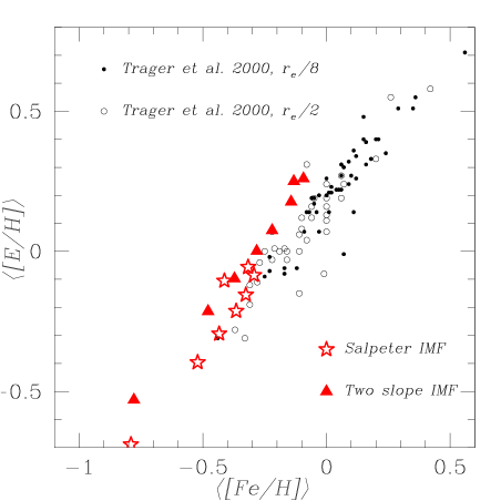
Very recently, Trager et al. (2000a) have derived single-burst stellar population equivalent ages, metallicities, and abundance ratios for a sample of local early-type galaxies from H, Mg, and Fe line strenghts using an extension of the Worthey (1994) models that accounts for the enhancements of Mg and other -elements relative to the Fe-peak elements. The metallicities and enhancement ratios [E/Fe] they have found are strongly peaked around +0.26 and +0.20, respectively, in an aperture of radius /8. Gradients in stellar populations within galaxies are found to be mild, with metallicity decreasing by 0.20 dex and [E/Fe] remaining nearly constant out to an aperture of radius /2 for nearly all systems. In Fig. 6 we compare our [E/H] vs. [Fe/H] relation for Models from 1b,d to 8b,d (spheroid masses range from to ; set b: Salpeter IMF, set d: two slope IMF) to that by Trager et al. (2000a,b). Results relevant to Models from 1c to 8c (single slope IMF flatter than the Salpeter) are very similar to those relevant to Models from 1d to 8d and therefore have not been plotted in the graph. As expected, our metallicities and abundance ratios agree much better with the Trager et al.’s ones computed through the global /2 aperture rather than with those computed through the central /8 aperture. Again, the discrepancy is mainly due to the fact that our abundances are accounting for the distribution of stellar populations over the whole galactic physical dimension. Besides this, a remarkable point is that the slope of our [E/H] vs. [Fe/H] relation is quite similar to that found by Trager et al. (2000a,b) for central values. The situation is also improving if galaxy formation is pushed at higher redshift (Table 4).
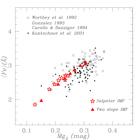
So far, we made an attempt to compare theoretical abundances for integrated early-type galaxies with estimates coming from the analysis of observed spectral indices. Now viceversa we want to use some calibrations and translate the theoretical abundance ratios into metallicity indices to be directly compared with observations. When dealing with early-type galaxies, the most widely used tool to compare theoretical predictions on -element and Fe abundances in stars to observations is the Mg2 vs. Fe diagram. In Fig. 7 observations (Worthey et al. 1992; González 1993; Carollo & Danziger 1994a,b; Kuntschner et al. 2001) are shown as long as model predictions. The theoretical indices have been obtained by converting the [Mg/Fe] and [Fe/H] ratios predicted by Models from 1b,d to 8b,d listed in Table 3 into the metallicity indices Mg2 and Fe by means of the calibrations by Tantalo et al. (1998), as described in Matteucci, Ponzone & Gibson (1998). The spread in the Mg2 data is reproduced remarkably well. In particular, the adoption of a two slope IMF of the kind of that described in Sect.3.1 allows us to cover a wider range of values in both indices. This is an unprecedent result, particularly interesting owing to the fact that an IMF of the kind adopted here is supported both observationally in the low-mass range (e.g., Wyse et al. 1999; Zoccali et al. 2000) and theoretically (Elmegreen 2000a,b). Note that an IMF with a single slope of 1.15 over the entire mass range would produce similar results. The high-mass end of the diagram, which is actually missed by our theoretical models, could be easily covered by adopting an Arimoto & Yoshii IMF, , i.e., an IMF with an even flatter slope. However, as we already noted before, an offset between model predictions and data has to be expected, since data refer to central index values, whereas model predictions are relevant to the whole physical dimension of the galaxy. Milone et al. (2000) find that the integrated indexes of their sample galaxies span a range from 0.2 to 0.3 in Mg2, and from 2 to 2.5 in Fe, while central index values range from 0.25 to 0.35 for Mg2, and from 2.5 to 3.5 for Fe. The offset we find is nearly the same (cfr. model predictions with data in Fig. 7). Moreover, as we already pointed out, in a monolithic picture for galaxy formation a natural cut-off in the stellar mass of galaxies should be expected, owing to the increase of the cooling time with increasing the host halo mass.
Finally, one could inquire about the properties of the very rare ellipticals formed at the highest redshifts, which are probably the hosts of the highest redshift QSOs ( 6). In Table 4 we summarize the results relevant to set d, for the case = 9 and = 0.4 Gyr.
4.2 Broad-band photometry
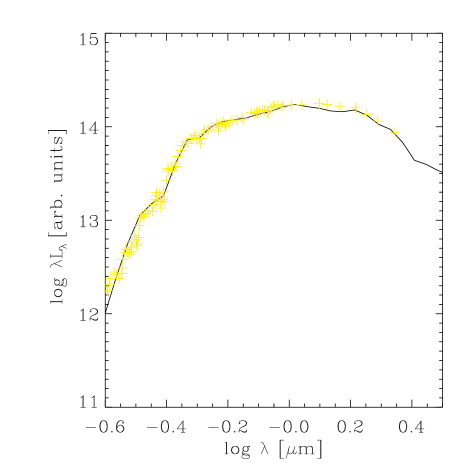
We have checked that also the photometric properties of our elliptical galaxy models are consistent with observations of local galaxies. To this aim, we have used the spectrophotometric code by Silva et al. (1998) and computed the spectral energy distribution (SED) and colours expected according to the star formation and chemical evolution histories of the models.
For the shape of the SED, an example is shown in Fig. 8, where we compare with the template SED for ellipticals by Arimoto (1996).
As discussed in Section 2.1, elliptical galaxies are observed to follow a CMR, with redder colours at increasing luminosity. The slope of this relation is interpreted as driven mostly by metallicity, rather than age, and its tightness as a small age dispersion among the bulk of the stellar populations. This interpretation rests on the reproduction, by several authors, of a combined set of observational constraints, including broad-band magnitudes and colours, spectral indexes, such as H, Mg2, Fe, etc., and abundance ratios (e.g., Bower et al. 1992; Bressan et al. 1994, 1996; Tantalo et al. 1996; Maraston & Thomas 2000). On the other hand, there are evidences, from this same data set for local galaxies and from higher- observations, that at least a minor fraction of the stellar populations of elliptical galaxies may have formed someway after the bulk of their stars was already formed (e.g., Bressan et al. 1996; Franceschini et al. 1998; Longhetti et al. 2000; Trager et al. 2000a,b).
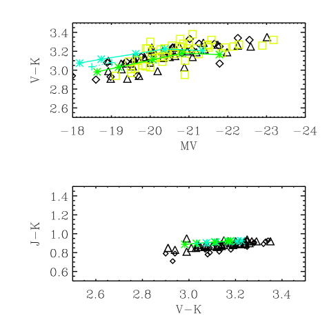
In Fig. 9, the colour – magnitude relation vs. and the vs. colours are shown for models of case (two slope IMF, Table 3) with mass at the age of 10 and 15 Gyr ( = 5 implies an age of 12 Gyr for the assumed cosmological parameters). Lower mass models, with prolonged star formations, have more prolonged evolutionary histories, for which we do not have enough constraints in the framework of our model. The colour is a strong function of the global metallicity of stars. In agreement with the results we found for the chemical abundances, the colours we obtain with the Salpeter IMF are too blue because of the very low metallicities reached (cases and in Table 3). Instead, in order to reproduce the observed colours, an average metallicity greater than solar must be reached, for the most massive models, which is the case for Models shown in Fig. 9. As remarked in the previous section, since the most massive objects in our model have , we do not cover the highest luminosity end of the plot. In Fig. 9 we also show the effect, for the two less massive objects in the plot at 15 Gyr, of a small burst episode involving 5 per cent of the mass, and taking place 4 Gyr ago. It is clear that the slope of the predicted CMR may fluctuate around the average value determined by metallicity because of these uncertainties.
The spectrophotometric code provides also the blue luminosities we need in order to compute the rates of Type Ia SNe at the present time. We find an average present SNIa rate varying from = 0.3 SNu for = 5 to = 0.2 SNu for = 9, to be compared with the observed value of 0.18 0.06 SNu (Cappellaro et al. 1999). Although uncertainties in both observations (e.g., empirical corrections for the bias in the inner galactic regions) and theory (e.g., fraction of stars of a given mass that enters the formation of binary systems which will give rise to Type Ia SN explosions; metallicity effects – which we do not account for here) prevent us from drawing any firm conclusion, we notice that theoretical results agree quite well with observations, at least at the 2 level.
4.3 The Ratio
While the luminous component of a galaxy is rather well defined, the associated halo is not easily identifiable as a well defined structure, separated from other close haloes. Nevertheless, luminous galaxies are good tracers of the mass distribution. Recent statistical studies of the weak lensing associated to nearby ‘lens’ galaxies allow for a first estimate of the galaxy-mass correlation function (McKay et al. 2001). These authors point out that the galaxy-mass correlation function is independent of the environment, confirming that the mass within 300 kpc from a central galaxy is clearly associated with the central object. They also find that elliptical galaxies in the luminosity range 1.6 17.7 1010 exhibit an average kpc . This result holds for dark matter haloes with isothermal density profile, while in the case of NFW profile the average value is about a half. Assuming a Salpeter IMF, our spectrophotometric model yields for elliptical galaxies with an age = 13 Gyr while, for the two slope IMF we adopted, . In the case of a NFW profile and km s-1 Mpc-1, the results obtained by McKay et al. (2001) suggest for a Salpeter IMF and 23 for the two slope IMF adopted in this paper, for galaxies with mass in the range 6 1010 – 6 10. From Fig. 10 it is apparent that in the mass interval explored the agreement between the results of McKay et al. (2001) and the model predictions is very good.

The increase of the ratio with decreasing mass in the low-mass range is due to the effect of the stellar feedback acting on the gas in shallow potential wells. This portion of the curve is sensitive to the fraction of the SN energy transferred to the gas, and to the IMF. As a result, the fraction of the baryons which form stars is strongly decreasing below a few 10, in keeping with observations showing that in low luminosity/mass galaxies the relative fraction of dark matter to stars progressively increases with decreasing luminosity (e.g., Persic, Salucci & Stel 1996).
At large masses the paroxysmal increase of the ratio with stellar mass is mainly due to the increase of the cooling time of the gas in the outer regions of large haloes. The fraction of baryons available for cooling and collapsing into stars is fixed by imposing [cfr. Eq.(8)]. The amount of stars formed is limited by the relatively short time lag between the virialization and the QSO appearance for massive objects. The ratio is not only sensitive to , but also to the formation redshift, larger masses being more easily assembled at high redshift, since at fixed mass the densities of DM and baryons increase with (see Section 2.1). In the case of = 9, the largest mass in stars in our set d with still acceptable is (Fig. 10). In this framework, more massive galaxies are assembled by coalescence, as suggested by their often observed distorted morphologies (e.g., double cores). On the other hand, the number density of massive haloes strongly decreases with increasing redshift. The result is the observed exponential decline of the luminosity/mass function at large luminosities/masses. The statistical aspects implied by these results will be discussed in a forthcoming paper.
It is worth noticing that the values of , namely the efficiency of reheating from SNeII, are significantly constrained by the results of McKay et al. (2001). If =1 is adopted, as it seems to be required in order to get, under very favorable hypotheses, 1 KeV of energy per particle injected into the IGM by SNe (Valageas & Silk 1999; Kravtsov & Yepes 2000), a minimum value of for and for the case d and = 5 is recovered. This value exceeds by a factor of 4 the result of McKay et al. (2001) for a NFW density profile.
5 Discussion and final remarks
In this work we concentrated mostly on the chemo-photometric properties of the stellar populations of early-type galaxies. In particular, we tested specific histories for the formation of the spheroids, which turned out to provide a good fit to crucial observed relations: the mass – metallicity relation, the Mg2 vs. Fe diagram, the colour – magnitude relation vs. , the vs. colours and the ratio. We found that all these properties are well reproduced by using the same dependence of the burst duration on galactic mass which is requested in order to fit the submillimetre source counts (Granato et al. 2001). It is worth noticing that the adopted scenario does hold for galaxies which are large enough to host a QSO, i.e., a few 109 , less massive objects possibly suffering for even more complex evolutionary paths than described above. Secondary episodes of star formation in massive galaxies at would produce only a tiny amount of stars; thus, the observed evolution of the FP and the observed [O II] emission could be explained (Treu et al. 2001) without any need of altering the global chemical properties of the stellar population.
At variance with most of the previous models of chemical evolution of spheroidal galaxies, we accounted for the stellar feedback through Eq.(13), i.e., we allowed a fraction of gas to be heated and subtracted to the ongoing star formation process at each time. The reheating term acts in the direction of reducing the efficiency of star formation in less massive spheroids. This reconciles our star formation efficiencies, decreasing with increasing galactic mass, with the increase of the star formation efficiency with increasing galactic mass required by other authors and it yields SFR . The overall result is similar, none the less the physical approach is very different. In our model, the star formation is governed by the rate at which baryonic gas cools and falls into DM haloes and is inhibited by heating from SNe and definitively ended by the QSO peak activity combined to the SN feedback.
We find that the ratios [Fe/H], [Mg/H], [Mg/Fe], [E/H], [E/Fe], and [Z/H] all increase with galactic mass (see Table 3). This is due to the combined effects of the following aspects of the model: i) the duration of star formation is shorter with increasing galactic mass; ii) the number of stellar generations increases with increasing galactic mass (SFR ); iii) the stellar feedback is more effective in low-mass galaxies (the amount of SNII-enriched material retained by low-mass galaxies is lower, due to the shallower potential wells).
If we relaxe the first hypothesis and set = 2 Gyr, constant with mass, the abundance ratios still increase with increasing galactic mass but [Mg/Fe] and [E/Fe], which flatten out (see also Kawata 2001). Therefore, a star-forming phase which lasts longer in less massive spheroids is strongly needed in order to reproduce the observed trend of increasing [Mg/Fe] in the nuclei of local ellipticals with increasing galactic mass. On the contrary, if we suppress the stellar feedback ( = 0), the ratios of all the elements with respect to hydrogen, [el/H], decrease with increasing mass, while the increase in [el/Fe] is preserved.
Flattening the IMF with increasing galactic mass is a further way of increasing the quantities [Fe/H], [Mg/H], [Mg/Fe], [E/H], [E/Fe], and [Z/H] with increasing galactic mass; however, in the framework of our model, we do not need such a flattening in order to increase the overall mean metallicity of the stellar population. A careful analysis of Tables 3 and 4 actually reveals that the mean metallicity of the stellar population starts slightly decreasing again at (cfr. the el/H abundance ratios for Models 1 and 2 in both tables). This is due to the increase of the cooling time of the gas in the outer regions of the largest virialized haloes. This increase limits the amount of stars which are born and hence the metal enrichment of the gas.

In the framework of the adopted model, massive QSO hosts () experience a relatively short ( 0.5 – 1 Gyr), intense (SFR 50 – 1000 yr-1) star-forming phase at high redshift ( 3), during which they show up as ultraluminous far-IR galaxies (SCUBA galaxies). After the shining of the QSO, they appear as EROs, for which we predict solar or higher than solar stellar metallicities. Moreover, we predict that very high rates of SNeIa should be observed in EROs, since in these objects the bulk of SNeIa explode soon after the shining of the QSO (see Fig. 11), in a dust-free medium. Therefore, non dusty EROs are preferred targets for searching for high- SNeIa.
Intermediate- and low-mass QSO hosts () are characterized by a more protracted starburst phase ( 1 – 2.5 Gyr) and show up as Lyman break galaxies (LBGs) at 3 (see also Granato et al. 2001). The curves relevant to Model 5b in the upper panels of Fig. 3 are representative of the history of star formation of a typical LBG; more generally, our models predict SFRs between 5 and 50 yr-1 for this kind of objects. These values agree quite well with recent estimates of the star formation activity in LBGs by Pettini et al. (2001). Moreover, our models predict a value of log(O/H) + 12 8.2 – 9.2 in the gas of LBGs at , strongly depending on the adopted redshift of galaxy formation and hence on the age of the stellar population. The lowest log(O/H) + 12 value we give is associated to a low-mass spheroid (Model 7) which started forming stars at and to a stellar population of age yr; the highest one is associated to a more massive spheroid (Model 4) which started forming stars at and to a stellar population of age yr. The lowest values we find agree well with the estimates by Pettini et al. (2001). This is quite reassuring, since their estimates refer to objects with virial masses of about 1010 , and Model 7 indeed refers to an object with virial mass (see Table 2). A more detailed study of LBGs will be the subject of a forthcoming paper.
The adopted model implies that the ratio between the final mass of the black hole responsible for the QSO activity and the mass of the host galaxy is not evolving with redshift, at variance with respect to semi-analytical models (Kauffmann & Haehnelt 2000). The most recent observations show a modest, if any, variation of this ratio with redshift (Kukula et al. 2001; see also the discussion in Granato et al. 2001).
The ratio predicted by the model depends significantly on the adopted value of , the efficiency of the transfer of the SN energy output to the ISM. A very good agreement with the findings of McKay et al. (2001), for galaxies in the mass range 6 1010 – 6 1011 , is found under the assumption 0.1. The combination of potential well and feedback makes the ratio increasing with decreasing mass. The assumption =1 is strongly ruled out in our model by the fact that the minimum ratio would be 4 times larger than that found by McKay et al. (2001).
This last result is also important in the context of the preheating of the IGM in galaxy groups and clusters. Actually, it has been suggested that with and under very favorable conditions, SNe can yield as much as 0.5 – 1 KeV per particle, thus bringing theoretical models of cluster formation into agreement with observations. However, this would contrast with the ratio found in galaxies. The supernovae are likely to be supplemented by some other heating mechanism (Balogh, Babul & Patton 1999; Valageas & Silk 1999; Wu et al. 2000; Kravtsov & Yepes 2000). In particular, Valageas & Silk propose high-redshift preheating of the IGM by radiation from quasars. It is quite natural that the mechanism which accounts for the required heating of the entire ICM affects also the evolution of its host.
In the context of the relationship between the QSO and the host galaxy, it is also worth noticing that the model predicts a metal abundance of the gas at the epoch of the QSO appearance in close agreement with the values inferred from the BELRs of high- QSOs.
In conclusion, the basic assumption of the model, namely that massive spheroidal galaxies evolve rapidly after the virialization of their haloes till their QSOs shine, is reinforced by the match of the model outcomes with the observed properties. In particular, in this paper we have shown that QSOs can play a major role in determing the observed chemo-spectrophotometric properties of spheroidal galaxies in a wide range of mass.
Acknowledgments
L. S. and L. D. thank Gian Luigi Granato for the substantial contribution to the spectrophotometric code used for this work and for enlightening discussions. We also thank the referee for several comments and suggestions that improved the presentation of this work.
References
- [] Almaini, O. et al., 2001, MNRAS, submitted (astro-ph/0108400)
- [] Aragon-Salamanca A., Ellis R.S., Couch W.J., Carter D., 1993, MNRAS, 262, 764
- [] Arimoto N., 1996, in Leitherer C., Fritze-von-Alvensleben U., Huchra J., eds, ASP Conf. Ser. Vol. 98, The Impact of Stellar Physics on Galaxy Evolution. ASP, San Francisco, p. 287
- [] Arimoto N., Yoshii Y., 1987, A&A, 173, 23
- [] Arimoto N., Matsushita K., Ishimaru Y., Ohashi T., Renzini A., 1997, ApJ, 477, 128
- [] Awaki H. et al., 1994, PASJ, 46, L65
- [] Balogh M.L., Babul A., Patton D.R., 1999, MNRAS, 307, 463
- [] Barger A.J., Cowie L.L., Sanders D.B., Fulton E., Taniguchi Y., Sato Y., Kawara K., Okuda H., 1998, Nature, 394, 248
- [] Barnes J.E., Hernquist L.E., 1991, ApJ, 370, L65
- [] Baugh C.M., Cole S., Frenk C.S., 1996, MNRAS, 283, 1361
- [] Bender R., Burstein D., Faber S.M., 1992, ApJ, 399, 462
- [] Bender R., Saglia R.P., Ziegler B., Belloni P., Greggio L., Hopp U., Bruzual G.A., 1998, ApJ, 493, 529
- [] Bernardi M., Renzini A., da Costa L.N., Wegner G., Alonso M.V., Pellegrini P.S., Rité C., Willmer C.N.A., 1998, ApJ, 508, L143
- [] Blain A.W., Smail I., Ivison R.J., Kneib J.-P., 1999, in Bunker A.J., van Breugel W.J.M., eds, ASP Conf. Ser. Vol. 193, The Hy-Redshift Universe: Galaxy Formation and Evolution at High Redshift. ASP, San Francisco, p. 425
- [] Borgani S., Governato F., Wadsley J., Menci N., Tozzi P., Lake G., Quinn T., Stadel J., 2001, ApJ, 559, L71
- [] Borys C., Chapman S., Halpern M., Scott D., 2001, MNRAS, submitted (astro-ph/0107515)
- [] Bower R.G., Lucey J.R., Ellis R.S., 1992, MNRAS, 254, 589
- [] Bressan A., Chiosi C., Fagotto F., 1994, ApJS, 94, 63
- [] Bressan A., Chiosi C., Tantalo R., 1996, A&A, 311, 425
- [] Bruzual G., Charlot S., 1993, ApJ, 405, 538
- [] Bryan G.L., Norman M.L., 1998, ApJ, 495, 80
- [] Bullock J.S. et al., 2001, MNRAS, 321, 559
- [] Buote D.A., 1999, MNRAS, 309, 685
- [] Buzzoni A., Gariboldi G., Mantegazza L., 1992, AJ, 103, 1814
- [] Cappellaro E., Evans R., Turatto M., 1999, A&A, 351, 459
- [] Carollo C.M., Danziger I.J., 1994a, MNRAS, 270, 523
- [] Carollo C.M., Danziger I.J., 1994b, MNRAS, 270, 743
- [] Cavaliere A., Menci N., Tozzi P., 1997, ApJ, 484, L21
- [] Charbonnel C., do Nascimento J.D., Jr., 1998, A&A, 336, 915
- [] Chiappini C., Matteucci F., Padoan P., 2000, ApJ, 528, 711
- [] Ciotti L., D’Ercole A., Pellegrini S., Renzini A., 1991, ApJ, 376, 380
- [] Cohen J.G., 2001, ApJ, in press (astro-ph/0107107)
- [] Concannon K.D., Rose J.A., Caldwell N., 2000, ApJ, 536, L19
- [] Daddi E., Cimatti A., Pozzetti L., Hoekstra H., Röttgering H.J.A., Renzini A., Zamorani G., Mannucci F., 2000, A&A, 361, 535
- [] Dickinson M., 1995, in Buzzoni A., Renzini A., Serrano A., eds, ASP Conf. Ser. Vol. 86, Fresh Views of Ellipticals Galaxies. ASP, San Francisco, p. 283
- [] Djorgovski S., Davis M., 1987, ApJ, 313, 59
- [] Dressler A., Lynden-Bell D., Burstein D., Davies R.L., Faber S.M., Terlevich R.J., Wegner G., 1987, ApJ, 313, 42
- [] Dunlop J.S., 2001, in Lowenthal J., Hughes D., eds, Deep millimeter surveys. World Scientific, in press (astro-ph/0011077)
- [] Eggen O.J., Lynden-Bell D., Sandage A.R., 1962, ApJ, 136, 748
- [] Eisenhauer F., 2001, in Tacconi L.J., Lutz D., eds, Starbursts: Near and Far, in press (astro-ph/0101321)
- [] Ellis R.S., Smail I., Dressler A., Couch W.J., Oemler A., Jr., Butcher H., Sharples R.M., 1997, ApJ, 483, 582
- [] Elmegreen B.G., 1999, ApJ, 517, 103
- [] Elmegreen B.G., 2000a, MNRAS, 311, L5
- [] Elmegreen B.G., 2000b, ApJ, 539, 342
- [] Evrard A.E., Henry J.P., 1991, ApJ, 383, 95
- [] Faber S.M., Burstein D., Dressler A., 1977, AJ, 82, 941
- [] Faber S.M., Worthey G., González J.J., 1992, in Barbuy B., Renzini A., eds, IAU Symp. 149, The Stellar Populations of Galaxies. Kluwer, Dordrecht, p. 255
- [] Faber S.M., Friel E.D., Burstein D., Gaskell C.M., 1985, ApJS, 57, 711
- [] Fabian A.C. et al., 2000, MNRAS, 318, L65
- [] Fabian A.C., Crawford C.S., Ettori S., Sanders J.S., 2001, MNRAS, 322, L11
- [] Fan X. et al., 2001, AJ, 122, 2833
- [] Ferrarese L., Merritt D., 2000, ApJ, 539, L9
- [] Franceschini A., Toffolatti L., Mazzei P., Danese L., de Zotti G., 1991, A&AS, 89, 285
- [] Franceschini A., Mazzei P., de Zotti G., Danese L., 1994, ApJ, 427, 140
- [] Franceschini A., Silva L., Fasano G., Granato G.L., Bressan A., Arnouts S., Danese L., 1998, ApJ, 506, 600
- [] Friaça A.C.S., Terlevich R.J., 1998, MNRAS, 298, 399
- [] Gebhardt, K. et al., 2000, ApJ, 539, L13
- [] Gibson B.K., 1997, MNRAS, 290, 471
- [] Gibson B.K., Woolaston E.J., 1998, in Friedli D., Edmunds M., Robert C., Drissen L., eds, ASP Conf. Ser. Vol. 147, Abundance Profiles: Diagnostic Tools for Galaxy History. ASP, San Francisco, p. 308
- [] Gilmore G., 2001, in Tacconi L.J., Lutz D., eds, Starbursts: Near and Far, in press (astro-ph/0102189)
- [] González J.J., 1993, PhD thesis, Univ. of California, Santa Cruz
- [] Granato G.L., Silva L., Monaco P., Panuzzo P., Salucci P., De Zotti G., Danese L., 2001, MNRAS, 324, 757
- [] Haehnelt M.G., Rees M.J., 1993, MNRAS, 263, 168
- [] Hamann F., Ferland G., 1999, ARA&A, 37, 487
- [] Hamann F., Korista K.T., Ferland G.J., Warner C., Baldwin J., 2001, ApJ, 564, 592
- [] Hughes D.H. et al., 1998, Nature, 394, 241
- [] Ikeuchi S., 1977, Prog. Theor. Phys., 58, 1742
- [] Im M. et al., 2001, ApJ, in press (astro-ph/0011092)
- [] Inoue S., Sasaki S., 2001, ApJ, 562, 618
- [] Ishimaru Y., Arimoto N., 1997, PASJ, 49, 1
- [] Jørgensen I., 1999, MNRAS, 306, 607
- [] Kaiser N., 1991, ApJ, 383, 104
- [] Kauffmann G., 1996, MNRAS, 281, 487
- [] Kauffmann G., Charlot S., 1998, MNRAS, 294, 705
- [] Kauffmann G., Haehnelt M., 2000, MNRAS, 311, 576
- [] Kauffmann G., White S.D.M., Guiderdoni B., 1993, MNRAS, 264, 201
- [] Kauffmann G., Guiderdoni B., White S.D.M., 1994, MNRAS, 267, 981
- [] Kawata D., 2001, ApJ, 558, 598
- [] Kobayashi C., Arimoto N., 1999, ApJ, 527, 573
- [] Kodama T., Arimoto N., Barger A.J., Aragon-Salamanca A., 1998, A&A, 334, 99
- [] Kormendy J., Richstone D., 1995, ARA&A, 33, 581
- [] Kravtsov A.V., Yepes G., 2000, MNRAS, 318, 227
- [] Kroupa P., 2001, in Grebel E., Brandner W., eds, ASP Conf. Ser., Modes of Star Formation and the Origin of Field Star Populations. ASP, San Francisco, in press (astro-ph/0102155)
- [] Kukula M.J., Dunlop J.S., McLure R.J., Miller L., Percival, W.J., Baum S.A., O’Dea C.P. 2001, MNRAS, 326, 1533
- [] Kuntschner H., 2000, MNRAS, 315, 184
- [] Kuntschner H., Davies R.L., 1998, MNRAS, 295, L29
- [] Kuntschner H., Lucey J.R., Smith R.J., Hudson M.J., Davies R.L., 2001, MNRAS, 323, 615
- [] Larson R.B., 1974a, MNRAS, 169, 229
- [] Larson R.B., 1974b, MNRAS, 173, 671
- [] Larson R.B., Tinsley B.M., 1974, ApJ, 192, 293
- [] Lilly S.J., Eales S.A., Gear W.K.P., Hammer F., Le Fèvre O., Crampton D., Bond J.R., Dunne L., 1999, ApJ, 518, 641
- [] Lloyd-Davies E.J., Ponman T.J., Cannon D.B., 2000, MNRAS, 315, 689
- [] Loewenstein M., Mathews W.G., 1991, ApJ, 373, 445
- [] Loewenstein M., Mushotzky R.F., Tamura T., Ikebe Y., Makishima K., Matsushita K., Awaki H., Serlemitsos P.J., 1994, ApJ, 436, L75
- [] Longhetti M., Bressan A., Chiosi C., Rampazzo R., 2000, A&A, 353, 917
- [] Magliocchetti M., Moscardini L., Panuzzo P., Granato G.L., De Zotti G., Danese L., 2001, MNRAS, 325, 1553
- [] Magorrian J. et al., 1998, AJ, 115, 2285
- [] Maller A.H., Dekel A., Somerville R.S., 2002, MNRAS, 329, 423
- [] Maraston C., Thomas D., 2000, ApJ, 541, 126
- [] Mathews W.G., Baker J.C., 1971, ApJ, 170, 241
- [] Matsumoto H., Koyama K., Awaki H., Tsuru T., Loewenstein M., Matsushita K., 1997, ApJ, 482, 133
- [] Matsushita K., Ohashi T., Makishima K., 2000, PASJ, 52, 685
- [] Matsushita K. et al., 1994, ApJ, 436, L41
- [] Matteucci F., 1992, ApJ, 397, 32
- [] Matteucci F., 1994, A&A, 288, 57
- [] Matteucci F., Greggio L., 1986, A&A, 154, 279
- [] Matteucci F., Padovani P., 1993, ApJ, 419, 485
- [] Matteucci F., Tornambè A., 1987, A&A, 185, 51
- [] Matteucci F., Ponzone R., Gibson B.K., 1998, A&A, 335, 855
- [] McCarthy P.J. et al., 2000, in Deep Fields, ESO Publications, in press (astro-ph/0011499)
- [] McKay T.A. et al., 2001, ApJ, submitted (astro-ph/0108013)
- [] McLure R.J., Dunlop J.S., 2001, MNRAS, 327, 199
- [] Merritt D., Ferrarese L., 2001a, ApJ, 547, 140
- [] Merritt D., Ferrarese L., 2001b, MNRAS, 320, L30
- [] Milone A., Barbuy B., Schiavon R.P., 2000, AJ, 120, 131
- [] Mobasher B., Guzman R., Aragon-Salamanca A., Zepf S., 1999, MNRAS, 304, 225
- [] Monaco P., Salucci P., Danese L., 2000, MNRAS, 311, 279
- [] Mushotzky R.F., Loewenstein M., Awaki H., Makishima K., Matsushita K., Matsumoto H., 1994, ApJ, 436, L79
- [] Navarro J.F., Frenk C.S., White S.D.M., 1996, ApJ, 462, 563
- [] Navarro J.F., Frenk C.S., White S.D.M., 1997, ApJ, 490, 493
- [] Nomoto K., Hashimoto M., Tsujimoto T., Thielemann F.-K., Kishimoto N., Kubo Y., Nakasato N., 1997, Nucl. Phys. A, 616, 79c
- [] O’Connell R.W., 1976, ApJ, 206, 370
- [] Pagel B.E.J., Patchett B.E., 1975, MNRAS, 172, 13
- [] Persic M., Salucci P., Stel F., 1996, MNRAS, 281, 27
- [] Peterson R.C., 1976, ApJ, 210, L123
- [] Pettini M., Shapley A.E., Steidel C.C., Cuby J.-G., Dickinson M., Moorwood A.F.M., Adelberger K.L., Giavalisco M., 2001, ApJ, 554, 981
- [] Ponman T.J., Cannon D.B., Navarro J.F., 1999, Nature, 397, 135
- [] Press W.H., Schechter P., 1974, ApJ, 187, 425
- [] Recchi S., Matteucci F., D’Ercole A., 2001, MNRAS, 322, 800
- [] Renzini A., Ciotti L., 1993, ApJ, 416, 49L
- [] Renzini A., Ciotti L., D’Ercole A., Pellegrini S., 1993, ApJ, 419, 52
- [] Roussel H., Sadat R., Blanchard A., 2000, A&A, 361, 429
- [] Salpeter E.E., 1955, ApJ, 121, 161
- [] Sheth R.K., Tormen G., 1999, MNRAS, 308, 119
- [] Silk J., Rees M.J., 1998, A&A, 331, L1
- [] Silva L., Granato G.L., Bressan A., Danese L., 1998, ApJ, 509, 103
- [] Smail I., Ivison R.J., Blain A.W., 1997, ApJ, 490, L5
- [] Smail I., Ivison R.J., Owen F.N., Blain A.W., Kneib J.-P., 2000, ApJ, 528, 612
- [] Stanford S.A., Eisenhardt P.R., Dickinson M., 1998, ApJ, 492, 461
- [] Sutherland R.S., Dopita M.A., 1993, ApJS, 88, 253
- [] Talbot R.J., Jr., Arnett W.D., 1973, ApJ, 186, 51
- [] Tantalo R., Chiosi C., Bressan A., Fagotto F., 1996, A&A, 311, 361
- [] Tantalo R., Chiosi C., Bressan A., 1998, A&A, 333, 419
- [] Terlevich A.I., Forbes D.A., 2001, MNRAS, submitted (astro-ph/0110413)
- [] Thielemann F.-K., Nomoto K., Hashimoto M., 1993, in Prantzos N., Vangioni-Flam E., Cassé M., eds, Origin and Evolution of the Elements. Cambridge Univ. Press, Cambridge, p. 297
- [] Thomas D., 1999, MNRAS, 306, 655
- [] Thomas D., Kauffmann G., 1999, in Hubeny I., Heap S., Cornett R., eds, ASP Conf. Ser. Vol. 192, Spectrophotometric Dating of Stars and Galaxies. ASP, San Francisco, p. 261
- [] Trager S.C., Faber S.M., Worthey G., González J.J., 2000a, AJ, 119, 1645
- [] Trager S.C., Faber S.M., Worthey G., González J.J., 2000b, AJ, 120, 165
- [] Treu T., Stiavelli M., Casertano S., Møller P., Bertin G., 2001, ApJ, 564, L13
- [] Valageas P., Silk J., 1999, A&A, 350, 725
- [] van den Hoek L.B., Groenewegen M.A.T., 1997, A&AS, 123, 305
- [] van der Marel R.P., 1999, AJ, 117, 744
- [] van Dokkum P.G., Franx M., Kelson D.D., Illingworth G.D., 1998, ApJ, 504, L17
- [] Voit G.M., Bryan G.L., 2001, Nature, 414, 425
- [] Warner C., Hamann F., Shields J.C., Constantin A., Foltz C.B., Chaffee F.H., 2001, ApJ submitted (astro-ph/0111002)
- [] Weiss A., Peletier R.F., Matteucci F., 1995, A&A, 296, 73
- [] Worthey G., 1994, ApJS, 95, 107
- [] Worthey G., 1998, PASP, 110, 888
- [] Worthey G., Ottaviani D.L., 1997, ApJS, 111, 377
- [] Worthey G., Faber S.M., González J.J., 1992, ApJ, 398, 69
- [] Wu K.K.S., Fabian A.C., Nulsen P.E.J., 2000, MNRAS, 318, 889
- [] Wyse R.F.G., Gilmore G., Feltzing S., Houdashelt, M., 1999, in Bunker A.J., van Breugel W.J.M., eds, ASP Conf. Ser. Vol. 193, The Hy-Redshift Universe: Galaxy Formation and Evolution at High Redshift. ASP, San Francisco, p. 181
- [] Yamada M., Fujita Y., 2001, ApJ, 553, L145
- [] Yoshii Y., Arimoto N., 1987, A&A, 188, 13
- [] Ziegler B.L., Bender R., 1997, MNRAS, 291, 527
- [] Zoccali M. et al., 2000, ApJ, 530, 418