Contribution of the Large Magellanic Cloud to the Galactic Warp

Abstract

Multi-scale interaction between the LMC, the Galactic halo, and the disk is examined with N-body simulations, and precise amplitudes of the Galactic warp excitation are obtained. The Galactic models are constructed most realistically to satisfy available observational constraints on the local circular velocity, the mass, surface density and thickness of the disk, the mass and size of the bulge, the local density of the halo matter at the solar radius, and the mass and orbit of the LMC. The mass of the halo within $R=50$ kpc is set to about $5\times 10^{11}M_{\odot}$. Since the observational estimate of the mass distributed in outer region has large ambiguity, two extreme cases are examined; $M(<170\mathrm{kpc})=2.1$ and $0.9\times 10^{12}M_{\odot}$. LMC is orbiting in a ellipse with apocentric radii of 100 kpc, thus the main difference between our two models is the mass density in the satellite orbiting region, so that our study can clarify the role of the halo on excitation of the warp.

By using hybrid algorithm (SCF-TREE) I have succeeded to follow the evolution with millions of particles. The orbiting satellite excites density enhancement as a wake, and the wake exerts a tidal force on the disk. Because of the additional torque from the wakes in the halo, the amplitudes of the induced warps are much larger than the classical estimate by hunt1969, who considered only the direct torque from the LMC. The obtained amplitudes of $m=0$, 1, 2 warps in the larger halo model show very good agreement with the observed amplitude in the Milky Way. This result revives the LMC as a possible candidate of the origin of the Galactic warp. Our smaller halo model, however, yield only weak warps in all the harmonic modes. Therefore the halo still has significant influence on excitation of warp even in the interaction scenario for excitation of warps.

1 Introduction

The origin of galactic disk warping, which is typically vertical bending of disks in a integral shape, is a long-standing problem. Even after 40 year efforts to explain the phenomena since the discovery of the warp in the Milky Way [burke1957, kerr1957], there is still no generally acceptable theory. A general review of the problem can be found in binn1992.

There are several observational facts that any convincing theory must explain. The first point is the longevity of the warps. Observations of neutral hydrogen layers [bosm1991] and stellar disks [sanc1990, resh1998] have revealed that about a half of spiral galaxies exhibit warps. Such high frequency of warps indicate that the warps are long-lived with about the same age as galaxies, otherwise some mechanism keeps exciting the warps. In both cases the warp excitation mechanism must be ubiquitous. The second point is the warp amplitude. For instance the Milky Way has a prominent warp and its amplitude is 2 kpc at Galactocentric distances $R\sim 14$ kpc[hend1982], and 4 kpc at $R\sim 20$ kpc [dipl1991]. The torque that can bend the disk in such a large amplitudes is so strong, which make it difficult to find the source of the torque [hunt1969]. The third point is alignment of the warp nodes. Most of spiral galaxies including our own have straight line of nodes within the Holmberg radius, and outward the lines of nodes make leading spirals [brig1990]. This fact presents a contrast to the spiral arms in the grand-design spiral.

Simple analysis [binn1992] shows that the simplest interpretation of the warp as a vertical oscillation of matters without considering selfgravity, is not working, because the line of nodes wind up in a time scale of 1 or 2 Gyr. Therefore self-consistent treatment is necessary. There are several hopeful theories, all of which have, however, some shortcomings.

The first step to understand long-lived warps is the normal mode analysis in steady state galaxies. hunt1969 showed that there are many bending normal modes in their thin-disk models, but unless density of the disks are cut-off sharply at their edges the frequency spectrum is at least partly continuous. In such disks any realistic perturbation would excite propagating wave packets, thus the warping wave is dispersed. A long-lived warp can correspond only to a discrete mode. If the disk is truncated at some radius, there is only one discrete normal mode, which is called a modified tilt mode [spar1988]. spar1988 showed that if disk is embedded in a flattened halo there is at most one discrete mode. Shapes of the mode show good agreement with observed warps, and even though the disk is not in the right shape of the modified tilt mode initially, it dynamically evolves to fit the mode [hofn1994].

The normal mode theory works very well as long as the halo is treated as a rigid body. However, once the self-consistent response of halo is included several problems emerge. For example, dynamical friction acting on the disk from the halo dissipates the warping motion [nels1995, dubi1995], and also the line of nodes often winds up tightly [binn1998a, idet2000]. To find the normal modes in fully self-consistent composite systems of a disk and a halo is extremely intractable.

One possible mechanism to keep the misalignment between a disk and a halo symmetric plane is continuous addition of matter with misaligned angular momentum to the halo. Inclined cosmic infall [ostriker-e1989, jian1999] might support the mechanism. jian1999 have shown that when infall reorientates the outer part of a galactic halo by several degrees per Gyr, a realistic warp is excited. Though the result seems appealing, their model of the infall is still too idealistic, and numerical studies are relatively short ($\sim$ 1 Gyr) to explain long-lived warps. Refined studies are necessary.

Another mechanism, which we are examining in this paper, is interaction with satellites. This mechanism is intuitively plausible because the most frequent $m=1$ warp is easily associated with a tidal field from a satellite. Furthermore increasing observational evidence suggests that most of the galaxies have satellite dwarfs. In fact, recently a faint dwarf companion has been discovered around NGC 5907, which was considered as a typical example of a warping galaxy without interacting companions [shan1998]. Also statistics show positive correlation between warping and existence of interacting companions [resh1998]

The only but severe problem of the interaction scenario is that the tidal forces from satellites are usually too small. For example, hunt1969 showed that the direct tidal force from the Large Magellanic Cloud (LMC) of $10^{10}M_{\odot}$ at 50 kpc can excite a warp with an amplitude at largest 100 pc at 16 kpc, while the real Galactic warp is about 3 kpc.

Against the problem, a remedy was proposed by wein1998c (hereafter W1998). Main point of his idea is to incorporate the halo response to the orbiting motion of a satellite into the source of the tidal forces. As the satellite moves, rotating density waves which have resonant frequencies to the satellite rotation are excited. In a nearly isothermal halo the most dominant wake appears at the position of 2:1 resonance, which is at about half distance to the satellite orbit. And the mass of the wake is about the same as the satellite, thus its tidal force is much larger than those from the satellite. W1998 showed with linear analysis for infinitely thin disks, that the tidal forces from the Large Magellanic Cloud (LMC) and its wake are large enough to excite the observable warp.

In order to prove this idea, fully self-consistent numerical simulations of three-dimensional disks are necessary. This is, in fact, very difficult and expensive, because we have to treat the small vertical motions of a very thin disk embedded in a very massive halo, which is extended well beyond the LMC orbit. W1998 estimated that 1 million particles are necessary to reduce numerical noise in order to distinguish meaningful dynamics of the disk.

This requirement is here accomplished by using a hybrid algorithm, TREE-SCF [vine1998], which particularly suits our problem of warping disk dynamics. Furthermore, we make the models as close to the real Milky Way – LMC system as possible, so that we can make precise evaluation of the warp amplitudes.

In section 2 we first describe by a brief summary the method to construct the Galaxy models using kuij1995, then give some parameters of the models which we use in this study. The precise input parameters in the kuij1995 codes are listed in the appendix. Section 3 explains algorithms and parameters of the TREE-SCF code. The results of the numerical simulations are given in Section 4. Section 5 is devoted to conclusion and discussions.

2 Galaxy Models

The aim of this study is to examine the influence of the LMC on excitation of the Galactic warp. Therefore we must first construct equilibrium Galaxy models that have no warp, and then put a satellite in the LMC orbit.

To construct equilibrium models for a multi-component system like the Milky Way is actually a hard task. Many galactic models are constructed with the assumptions that the halo and bulge are static backgrounds, or assuming that velocity distribution is Gaussian and solving only the Jeans equations. The deviation of these approximations from a true equilibrium causes initial transient behavior, in other words relaxation into the true equilibrium. That behavior changes the initial distribution especially in the disk. In the disk warping problem it is necessary to avoid any disturbance on the disk other than that from the satellite.

A suitable initial model is given by kuij1995 (hereafter KD1995), which is nearly an exact solution of the collisionless Boltzmann and Poisson’s equations. In their method, the configurations of a halo, bulge, and disk are given by means of distribution functions which depend only on integrals of motion. By the Jeans theorem such distribution functions are already steady state solutions of the collisionless Boltzmann equation. Densities can be calculated from the distribution functions, which depend on the positions only through the potential function. Therefore the main task is to determine the functional form of the potential by solving Poisson’s equation numerically.

The halo distribution function takes the form

$$f_{\mathrm{halo}}(E,L_{z}^{2})=\left\{\begin{array}[]{ll}\left[(AL_{z}^{2}+B)\exp(-E/\sigma_{0}^{2})+C\right]\left[\exp(-E/\sigma_{0}^{2})-1\right]&\mathrm{if}E<0,\\ 0&\mathrm{otherwise},\\ \end{array}\right.$$ (1)

where $L_{z}$ is the specific angular momentum about the axis of symmetry, and $E$ is the relative energy, which is defined so that $E=0$ at the edge of the distribution (where $\rho=0$)[binn1987]. This distribution function has five free parameters: the potential at the center $\Psi_{0}$, which appears implicitly through the definition of the relative energy, the velocity scale $\sigma_{0}$, and three factors $A$, $B$, and $C$. This distribution is based on Evans’s model, which has axisymmetric logarithmic potential, but is truncated at a finite radius by lowering the distribution function in the same manner as the lowered isothermal models. The factors $A$ and $B$ control the system flattening ($q$) and the core radius ($R_{c}$), respectively, and all the three factors are scaled by the density scale ($\rho_{1}$).

The bulge distribution function is the same as a King model [binn1987] and has the form

$$f_{\mathrm{bulge}}(E)=\left\{\begin{array}[]{ll}\rho_{\mathrm{b}}(2\pi\sigma_{\mathrm{b}}^{2})^{-3/2}\exp[(\Psi_{0}-\Psi_{\mathrm{c}})/\sigma_{\mathrm{b}}^{2}]&\{\exp[-(E-\Psi_{\mathrm{c}})/\sigma_{\mathrm{b}}^{2}]-1\}\\ &\mbox{if }E<\Psi_{\mathrm{c}},\\ 0&\mbox{otherwise}.\end{array}\right.$$ (2)

This distribution has 3 parameters. $\Psi_{\mathrm{c}}$ is the cutoff potential, $\rho_{\mathrm{b}}$ the central bulge density, and $\sigma_{\mathrm{b}}$ the bulge velocity dispersion.

For these two distributions, the densities are given by analytic functions of $R$ and $\Psi$ [kuij1995].

The disk distribution must depend on 3 integrals of motion, in order to keep the triaxial velocity ellipsoid in the disk [dehn1998c]. The third integral is, however, not known as any analytical function, so that distribution function cannot be written as an analytical function. For the sake of convenience, an approximated distribution function is employed which depends on the energy in the vertical oscillations, $E_{z}\equiv\Psi(R,z)-\Psi(R,0)+\frac{1}{2}v_{z}^{2}$, and that in planer motion, $E_{\mathrm{p}}\equiv E-E_{z}$, as well as $L_{z}$. $E_{z}$ is quite well conserved for stars in nearly circular orbits. The form is

$$f_{\mathrm{disk}}(E_{\mathrm{p}},L_{z},E_{z})=\frac{\Omega(R_{\mathrm{c}})}{(2\pi^{3})^{1/2}\kappa(R_{\mathrm{c}})}\frac{\tilde{\rho_{\mathrm{d}}}(R_{\mathrm{c}})}{\tilde{\sigma_{R}}^{2}(R_{\mathrm{c}})\tilde{\sigma}_{z}(R_{\mathrm{c}})}\exp\left[-\frac{E_{p}-E_{\mathrm{c}}(R_{\mathrm{c}})}{\tilde{\sigma}_{R}^{2}(R_{\mathrm{c}})}-\frac{E_{z}}{\tilde{\sigma}_{z}^{2}(R_{\mathrm{c}})}\right]$$ (3)

where $R_{\mathrm{c}}$ and $E_{\mathrm{c}}$ are the radius and energy of a circular orbit with angular momentum $L_{z}$, and $\Omega$ and $\kappa$ are the circular and epicyclic frequencies at radius $R_{\mathrm{c}}$. The ‘tilde’ functions $\tilde{\rho_{\mathrm{d}}}$, $\tilde{\sigma}_{R}$, and $\tilde{\sigma}_{z}$ are free functions. Therefore the density and the radial velocity dispersion are conveniently selected as

$$\rho_{\mathrm{disk}}(R,z)=\frac{M_{\mathrm{d}}}{8\pi R_{\mathrm{d}}^{2}z_{\mathrm{d}}}\mathrm{e}^{-R/R_{\mathrm{d}}}\mathrm{erfc}\left(\frac{r-R_{\mathrm{out}}}{\sqrt{2}\delta R_{\mathrm{out}}}\right)\exp\left[-4.6187\frac{\Psi_{z}(R,z)}{\Psi_{z}(R,3z_{\mathrm{d}})}\right],$$ (4)

and

$$\tilde{\sigma}_{R}^{2}=\sigma_{R}^{2}(0)\exp(-R/R_{\mathrm{d}}).$$ (5)

$\tilde{\rho_{\mathrm{d}}}$ and $\tilde{\sigma}_{z}$ are iteratively adjusted so that the densities on the mid-plane and at height $z=3z_{\mathrm{d}}$ will agree with those given by eq. (4). The distribution of the disk has 6 free parameters: the disk mass, $M_{\mathrm{d}}$, the radial scale length $R_{\mathrm{d}}$, the vertical scale height $z_{\mathrm{d}}$, the disk truncation radius $R_{\mathrm{out}}$, the truncation width $\delta R_{\mathrm{out}}$, and the central velocity dispersion of the disk $\sigma_{R}(0)$.

kuij1995 also give a numerical program to calculate the distribution functions and densities. Their algorithm consists of the following 4 steps. (i) A test potential function $\Psi^{(0)}(R,z)$ is given. (ii) The potential is substituted into the density functions which are calculated from the distribution functions. (iii) Poisson’s equation is solved by using pren1970’s method to determine a new potential functions. (iv) The procedure 2 and 3 are repeated until the potential functions have converged.

By using kuij1995’s method, we construct the Galaxy models which satisfy observational properties. We apply the following constraints;

• solar radius : $R_{0}$ = 8 kpc

• circular velocity of the disk at the solar radius : $V_{\mathrm{c}}=220$ km/s

• total surface density within 1.1 kpc of the disk plane :

  $\Sigma_{1.1}(R_{0})=71\pm 6M_{\odot}\mathrm{pc}^{-2}$ [kuij1991b]

• contribution of the disk material to $\Sigma_{1.1}$ :

  $\Sigma_{\mathrm{d}}(R_{0})=48\pm 9M_{\odot}\mathrm{pc}^{-2}$ [kuij1991b]

• total Galaxy mass within 50 kpc :

  $M_{\mathrm{tot}}(<50\mathrm{kpc})=5.4^{+0.2}_{-3.6}\times 10^{11}M_{\odot}$ [wilk1999]

• total Galaxy mass within 170 kpc :

  $M_{\mathrm{tot}}(<170\mathrm{kpc})=1.9^{+3.6}_{-1.7}\times 10^{12}M_{\odot}$ [wilk1999]

• the halo is spherical : $q=1.0$, i.e., $A=0$ [ibat2001]

Moreover, we assume that

• disk mass is $5\times 10^{10}M_{\odot}$,

• disk scale length is 3.2 – 3.5 kpc,

• disk scale height is 200 – 250 pc,

• disk edge is 25 – 28 kpc,

• bulge mass is 15% of that of the disk,

• and bulge size is about 2 kpc.

Table 1: Sizes of the components in the Galaxy models, which are used in this paper

	Model L		Model S
	mass ($M_{\odot}$)	radius	mass ($M_{\odot}$)	radius
Disk	$5\times 10^{10}$	3.2kpc	$5\times 10^{10}$	3.5kpc
Scale height		224pc		245pc
Disk edge		25.6kpc		28kpc
Bulge	$0.76\times 10^{10}$	2.21kpc	$0.75\times 10^{10}$	2.38kpc
Halo	$5.11\times 10^{12}$	1539kpc	$8.59\times 10^{11}$	262kpc

The halo mass and extent is very important, because in Weinberg’s scenario, the halo plays an important role as a mediator between a satellite and a disk. Observational estimate of the halo mass has, however, a huge error, so that we examine two extreme cases: one with the largest halo (Model L), and the other with the smallest possible halo (Model S). Construction of these models is made by KD1995’s code, which is available in their web site, and the input parameters are listed up in Appendix A. Some characteristic parameters for the two models are given in Table 1. The disk scale height and the edge radius are similar in both models. The disk surface densities for the model L and S are $\Sigma_{\mathrm{d}}(R_{0})=$ 45.3 and 45.5 $M_{\odot}\mathrm{pc}^{-2}$, while the total surface densities including halo contribution $\Sigma_{1.1}(R_{0})=$ 65.0 and 69.8 $M_{\odot}\mathrm{pc}^{-2}$, respectively. The halo masses for the model L and S are $M_{\mathrm{tot}}(<50\mathrm{kpc})=$ 5.58 and 4.93 $\times 10^{11}M_{\odot}$, and $M_{\mathrm{tot}}(<170\mathrm{kpc})=$ 2.1 and 0.9 $\times 10^{12}M_{\odot}$, respectively. The determination of the parameters was done by manual searching of the input parameters. Those are not unique solutions, because the parameter space of the KD1995’s model is larger than the number of the constraints. The model L and S are the first best fitted distributions. The bulge and halo radii listed in the table are the tidal radii, where their densities fall to zero. For model L, such a large tidal radius is necessary to ensure that the halo profile is nearly isothermal beyond the LMC orbit ($\sim 100$ kpc).

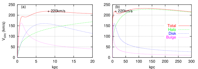
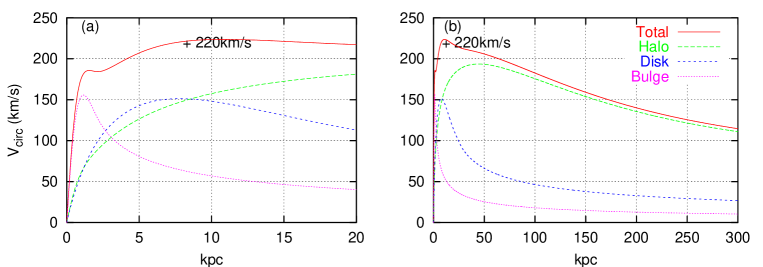
Figure 1: Circular velocity profiles for the model L. Panel (a) shows a small scale profile, and (b) shows a larger scale profile. The cross sign (+) shows the observational circular velocity at the solar radius.

Figure 2: Circular velocity profiles for the model S. Panel (a) shows a small scale profile, and (b) shows a larger scale profile. The cross sign (+) shows the observational circular velocity at the solar radius.

Figures 2 and 2 show the circular velocity profiles of the Model L and S, respectively. Within the disk extent, the circular velocity profiles are almost the same in the both models, but in outer regions where the LMC is orbiting, the model L still maintains flat rotation, whereas the model S is nearly Keplerian. The velocity dispersion profiles of the disk for the model L and S are shown in Fig. 3 (a) and (b), respectively. Both profiles are almost the same. The model velocity dispersions at the solar radius, $(\sigma_{R},\sigma_{\theta},\sigma_{z})\sim(41,29,13)$ km/s, are closer to those of the thin disk, and Toomre’s Q value has the minimum (1.7 for the model L, and 1.86 for the model S) around the solar radius.

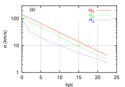
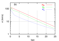
Figure 3: Velocity dispersion profiles of the disk. Panel (a) shows the model L and (b) the model S. Three curves correspond to the radial ($R$), azimuthal ($\theta$), and vertical ($z$) components.

Dynamical and numerical stability of the models are shown in Sec. 4.1.

We treat the LMC rather simply. It is modeled as an extended single particle with a spherical Hernquist profile,

$$\rho(r)=\frac{M_{\mathrm{LMC}}r_{0}}{2\pi r(r+r_{0})^{3}},$$ (6)

where the scale length is chosen to $r_{0}=3.2$ kpc, then the half mass radius is 7.7 kpc. The mass of the LMC is set to $M_{\mathrm{LMC}}=10.6\times 10^{9}M_{\odot}$, which is twice of the present LMC mass estimated by alve2000. This large mass includes contribution from the SMC, which is about 10% of the LMC, and the mass which is possibly stripped by tidal field from the Milky Way, during a period of 6 Gyr.

We need to trace the evolution of the Milky Way – LMC system, at least 6 Gyr to examine the warp dynamics, but it is very difficult to predict the orbital parameters of the LMC 6 Gyr ago. mura1980 have made a parameter survey with simple assumptions and found that the LMC has been revolving around the Milky Way in an eccentric orbit accompanied by the SMC. The present position of the LMC is nearly at a pericenter. With its kinematical data [krou1997a], the orbital plane of the LMC is determined. As a realistic assumption of the LMC orbit, we put the satellite in the present orbital plane at a distance of 112 kpc for the model L and 97 kpc for the model S. Only tangential velocity is given so that the initial position will be at apocenter and the eccentricity is 0.34 and 0.24 for the model L and S, respectively. As shown in Fig. 11, the satellite sinks to below 50 kpc at a pericenter after 6 Gyr. Since our halo is nearly spherical, the satellite remains in the initial orbital plane.

3 Numerical Methods

3.1 A hybrid $N$-body code

Numerical simulations for our problem require very large computational power because of its huge dynamical ranges. One important requirement is to keep the disk thin enough to distinguish subtle disk vertical dynamics. Artificial 2-body relaxation is the main source of harmful, i.e. undesired and unphysical heating. In order to reduce this effect a large number of particles is necessary. In particular, the relaxation among the disk particles is very large, because the velocity dispersions are small. Simple application of Chandrasekhar’s relaxation formula [binn1987] reads

$$T_{\mathrm{relax}}=\frac{4.2\times 10^{14}\mathrm{years}}{\ln\Lambda}\left(\frac{\sigma}{20\mathrm{km/s}}\right)^{3}\left(\frac{m}{M_{\odot}}\right)^{-2}\left(\frac{n}{\mathrm{pc}^{3}}\right)^{-1},$$ (7)

where $\Lambda$ is the Coulomb logarithm, and $\sigma$, $m$, and $n$ are velocity dispersion, mass, and number density of stars. The critical particle number in numerical simulations is $10^{6}$, with which the relaxation time is $\sim 10^{10}$ years.

For the halo, internal relaxation is no problem, because it is much hotter than the disk. However, a problem is that the halo is 100 times more massive than the disk in the model L. Even small noises of the halo could cause big influence on the disk or the satellite. To reduce the noise, a large particle number is necessary.

Another difficulty in our simulations is the huge difference in spatial scales and also in dynamics between the disk and the halo. The most important feature in the disk is delicate vertical motion, while the most interesting features in the halo are large scale wakes, which are excited by the satellite motion. It is of course possible to treat the system with a single scheme $N$-body code, like a tree-code, but another possibility is to deal with the disk and the halo by separate algorithms.

A hybrid $N$-body code, which seems suitable for our system, is the SCF-TREE code [vine1998]. The disk and bulge are represented by tree particles (e.g., barn1986), while the halo is treated by a method expanding the potential using bi-orthogonal polynomial series, which is widely known as SCF (Self-Consistent Field) method [clut1973, hernq1992, saha1993].

A tree code is a rather popular method for general $N$-body problems, because of its flexibility of system configuration and relatively high force resolution, which is controlled by softening lengths. The whole computational space is divided into nested cubic cells to form a hierarchical tree structure. Interaction between close particles is calculated by direct summation, but contribution from distant particles is calculated only as a group of particles contained in a large cell. This grouping is made with a simple criterion,

$$\theta>\frac{s}{d},$$ (8)

where $s$ and $d$ are the size and the distance of the grouped cell. $\theta$ is a control parameter, which is known as the tolerance parameter. With this grouping the number of calculations reduces to $\mathcal{O}(N\log N)$ (e.g., barn1986).

A SCF code is, on the other hand, an expansion method for calculation of gravitational forces. In the code density and potential are represented by a bi-orthogonal set of basis functions.

$$\rho(\mathbf{r})=\sum_{nlm}A_{nlm}\rho_{nlm}(\mathbf{r}),\quad\mbox{and}\quad\Phi(\mathbf{r})=\sum_{nlm}A_{nlm}\Phi_{nlm}(\mathbf{r}),$$ (9)

where each pair $\rho_{nlm}$ and $\Phi_{nlm}$ satisfies Poisson’s equation

$$\nabla^{2}\Phi_{nlm}=4\pi G\rho_{nlm},$$ (10)

and bi-orthogonal relations

$$\int\rho_{nlm}(\mathbf{r})[\Phi_{n^{\prime}l^{\prime}m^{\prime}}(\mathbf{r})]^{\ast}d\mathbf{r}=I_{nl}\delta_{nn^{\prime}}\delta_{ll^{\prime}}\delta_{mm^{\prime}},$$ (11)

where $I_{nl}$ are normalization factors.

The basic procedure of the SCF method is that first $N$ particles are distributed to sample the density, then the coefficients $A_{nlm}$ are calculated by expanding the density distribution. The potential is determined by the latter equation of (9), thus forces can be calculated at any position. The particle positions are thus advanced to the next time step.

The major advantage of the SCF method is that the speed of the computation scales as $\mathcal{O}(N)$, which is a smaller burden in increasing particle number than those of the direct summation method ($\mathcal{O}(N^{2}$)) or usual tree methods ($\mathcal{O}(N\log N)$).

A fundamental property of the SCF, which is particular among other expansion methods, is that each particle contributes not as a local gravitational source (that is so in other expansion methods), but on global modes of density distribution, so that there is no particle-particle interaction in the method. On the other words it is more suitable for study of the mode interactions. In our problem the most important dynamics in the halo is dynamical friction on the satellite. The classical picture of dynamical friction is due to scattering of field particles as a 2-body problem [chan1943, binn1987]. However, modern understanding of dynamical friction is rather due to interaction between the massive object and wave modes in the field [trema1984]. Therefore it seems reasonable to treat the halo by the SCF method.

In practical computation, the expanded series in eq. (9) should be truncated in a small number of terms. Since computational time is proportional to the number of terms, it is the most important for the SCF method to find a good basis functions which can fit the system distribution well with the lowest order term. There are several basis sets introduced in the literature [clut1973, hernq1992, saha1993, syer1995, earn1996, robi1996, zhao1996], but it is still terribly difficult to deal with a complex system like a disk galaxy.

The SCF-TREE code has strategic advantages more than compromise in our problem. By using a tree method the disk and bulge enjoy high resolution and flexibility to possibly large changes in their shape. We do not need so high resolution in the halo, but large number of particles are necessary to reduce noise, and the wave modes which are excited by the satellite motion should be solved correctly. Both requirements are perfectly accomplished by using the SCF method.

3.2 Parameter Specification

Our numerical code is fundamentally the same as vine1998. The tree part is based on hernq1987’s algorithm, and for the SCF part [hereafter HO]hernq1992’s basis set is incorporated. There are 7 steps in the calculations at each time-step:

1. Calculate the coefficients $A_{nlm}$ of the terms in the SCF expansion.

2. Build the tree from all the tree particles.

3. Calculate accelerations of TREE and SCF particles by the SCF expansion.

4. Form the tree interaction lists among TREE particles, and calculate accelerations of TREE particles by the tree system.

5. Form the tree interaction lists between SCF particles and TREE particles, and calculate accelerations of SCF particles by the tree system.

6. Calculate gravitational force from the satellite on all the TREE and SCF particles. Acceleration of the satellite is simultaneously calculated.

7. Update positions and velocities of all particles and the satellite.

We use a common time step for all particles, and the time integration scheme is the Leap-Frog. The time steps are fixed to 0.75 Myr and 0.875 Myr for the model L and S, respectively. These time steps are one fourth of the central free fall time, $T_{\mathrm{ff}}\equiv\frac{1}{4}\sqrt{3\pi/(2G\rho_{0})}\approx 3$Myr, which is the shortest time scale in the system. The time resolution at the center is marginal, but in most part of the disk the time step is an order of magnitude smaller than the vertical crossing time of the disk.

In the TREE part, $2^{19}(=512\mathrm{k})$ particles are used in total, and 448k and 64k particles are assigned to the disk and bulge, respectively. They have the same mass among each component, and mass ratio between the disk and bulge particles is $m_{\mathrm{bulge}}/m_{\mathrm{disk}}=1.05$. All particles have a single fixed softening length $r_{\varepsilon}\approx 50$ pc, which is $1/8$ of the disk initial thickness. The tolerance parameter is set to $\theta=0.7$, which is applied to TREE-TREE and also TREE-SCF interaction lists. In force calculation, up to quadrupole moments are included.

For the SCF calculations, choice of basis set is the most important. We employ the HO basis set. Justification of this choice is shown below.

The angular dependence of $\rho_{nlm}$ and $\Phi_{nlm}$ is expanded in the spherical harmonics,

$$\rho_{nlm}(\mbox{\boldmath$r$};\mathbf{r}) \equiv \sqrt{4\pi}\tilde{\rho}_{nl}(r)Y_{lm}(\theta,\phi)$$ (12)

$$\Phi_{nlm}(\mbox{\boldmath$r$}) \equiv \sqrt{4\pi}\tilde{\Phi}_{nl}(r)Y_{lm}(\theta,\phi),$$ (13)

where

$$Y_{lm}(\theta,\phi)=\sqrt{\frac{2l+1}{4\pi}\frac{(l-|m|)!}{(l+|m|)!}}P_{l}^{|m|}(\cos\theta)e^{im\phi}\times\left\{\begin{array}[]{ll}(-1)^{m}&(m\geq 0)\\ 1&(m<0)\end{array}\right.,$$ (14)

and the radial functions are expanded by using the Gegenbauer (Ultraspherical) polynomials,

$$\tilde{\rho}_{nl}(r) \equiv \frac{4n(n+2l+2)+(2l+1)(2l+3)}{4\pi r_{0}^{2}}\frac{\tilde{r}^{l}}{(1+\tilde{r}^{2})^{l+5/2}}C_{n}^{(l+1)}(\xi),$$ (15)

$$\tilde{\Phi}_{nl}(r) \equiv -\frac{\tilde{r}^{l}}{(1+\tilde{r}^{2})^{l+1/2}}C_{n}^{(l+1)}(\xi),$$ (16)

where

$$\tilde{r}\equiv\frac{r}{r_{0}},\quad\quad\xi\equiv\frac{\tilde{r}^{2}-1}{\tilde{r}^{2}+1},$$ (17)

and the convention $G=1$ is adopted. The pair of zeroth order terms in this expansion has the form

$$\rho_{000}=\frac{1}{2\pi}\frac{1}{\tilde{r}(1+\tilde{r})^{3}},\quad\Phi_{000}=-\frac{1}{1+\tilde{r}},$$ (18)

which is known as the Hernquist profile [hernq1990a]. This profile is introduced to fit the light curves of elliptical galaxies. It has a density cusp at the center, while there is no cusp in our halo model. This discrepancy causes bad fitting of the basis set in the central region. Except for that, the expansion with relatively small number of terms reproduces the original distribution very well. Figure 5 and 5 show the results of the expansion with the number of the radial terms 8 for the model L, and 9 for the model S, respectively. The scale lengths of the basis set are $r_{0}=115$ kpc for the model L, and $r_{0}=21$ kpc for the model S, respectively. In both figures the red solid lines show the original volume density profiles of the models averaged over spherical shells, and the blue dashed lines show those reproduced by truncated expansion of the HO basis set. Even with this small number of terms, the reproduced densities fit the originals fairly well from $r=0.3$ kpc to nearly the end of the halo extent. The largest discrepancy appears at the center, where the halo component gives the smallest contribution. The density of the expanded series becomes comparable to that of the bulge only within 10 pc from the center. We believe that this difference has no effect on the warping motion at $R\gtrsim 10$ kpc. In fact we found no noticeable structural change at the center in our test simulations owing to the difference of the SCF densities from the original equilibrium distribution.

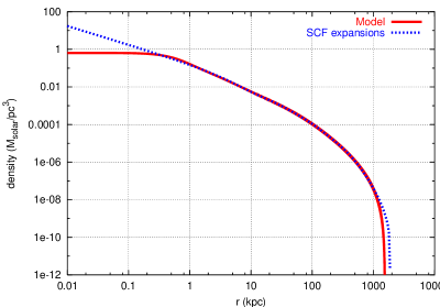
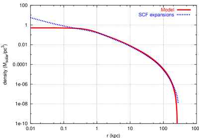
Figure 4: Spherically averaged density profile for the halo of the model L, and its SCF expansion with the scale length of the basis set $r_{0}=115$ kpc. Expansion is truncated after $n=8$ term.

Figure 5: Spherically averaged density profile for the halo of the model S, and its SCF expansion with the scale length of the basis set $r_{0}=21$ kpc. Expansion is truncated after $n=9$ term.

Other than the HO basis set, there are several different basis sets proposed for the purpose of galactic dynamics, including ones with a finite central core in density profiles. The most well-known example of the ‘cored’ profile is that based on the Plummer distribution. In this profile, however, density falls very quickly with increasing radius ($\propto r^{-5}$), therefore the Plummer basis set gives much worse fitting to our halo profile. In addition, zhao1996 gives a more general class of the basis sets, which include HO and the Plummer basis sets, but the only profile that has a central core is the Plummer profile. Therefore the HO basis set seems the best within our knowledge.

Even though the unperturbed halo distribution is approximated well by small number of the radial functions, the number of terms that is indeed necessary in our simulations is determined so that the density perturbations induced by the LMC should be also well approximated. We have made several test calculations with increasing the radial and angular functions with the presence of the LMC, which is reported in the next section. We judge the suitable number of terms by examining the satellite sinking, and select the number of the radial and angular functions, $n=8$ and $l=12$, respectively. Including more terms does not affect the satellite sinking history.

The center of the expansion of the SCF basis set is adjusted to the center of mass of the most tightly bound particles. By using an energy criterion, about one third of the total halo particles are used to determine the center of the expansion.

The number of particles that is used to sample the halo density is $2^{19}$. Therefore we use in total $2^{20}$ particles in the Galaxy in addition to one extended particle for the satellite. All simulations are made on Pentium III – Linux workstations (800MHz). Typical calculation time is 260 seconds per time step and in total about 500 hours to complete the evolution up to 6 Gyr. More than 60% of the CPU time is used in the TREE part.

4 Simulations

4.1 Stability of the Galaxy models

First we examine the stability of our Galaxy models. Without a satellite, these models must be stable and exhibit no warping motion. Moreover we have to check the validity of our numerical code. Thus the Galaxy models are constructed as described in Sec. 2 with in total $2^{20}$ particles, and their evolution is calculated with the SCF-TREE.

In order to characterize the disk evolution, we make a modal analysis both of the disk surface density and of the vertical distribution of the particles. For the disk surface density, $\Sigma(R,\phi)$, angular dependence is decomposed into the Fourier series,

$$\Sigma(R,\phi)=\Sigma_{0}(R)+\sum_{m=1}^{\infty}\Sigma_{m}(R)\cos(m|\phi-\psi_{m}(R)|).$$ (19)

Numerically, the disk particles are binned into annuli, $R\in[R^{(k-1)},R^{(k)}]$, where

$$0\leq R^{(1)}\leq R^{(2)}\leq\ldots\leq R^{(k)}\leq\ldots\leq R^{(K)},$$ (20)

then averaged coefficients in the annuli are calculated as follows;

$$\overline{\Sigma}_{0}^{(k)} = \frac{1}{\Delta S^{(k)}}\sum_{R^{(k-1)}<R_{i}<R^{(k)}}m_{i},$$

$$\overline{\Sigma}_{m}^{(k)}\cos(\psi_{m}) = \frac{2}{\Delta S^{(k)}}\sum_{R^{(k-1)}<R_{i}<R^{(k)}}m_{i}\cos(m\phi_{i}),$$ (21)

$$\overline{\Sigma}_{m}^{(k)}\sin(\psi_{m}) = \frac{2}{\Delta S^{(k)}}\sum_{R^{(k-1)}<R_{i}<R^{(k)}}m_{i}\sin(m\phi_{i}),$$

where $\Delta S^{(k)}\equiv\pi\{(R^{(k)})^{2}-(R^{(k-1)})^{2}\}$ is the area of the $k$th annulus, and $m_{i}$, $R_{i}$ and $\phi_{i}$ are the mass, radius in the disk plane and azimuth of the $i$-th particle.

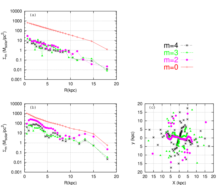
Figure 6: Modal analysis of the disk surface density profile for the model L. The panel (a) shows the coefficients of the modes $m=0$, 2, 3, 4 at the initial time. The panel (b) is the same as (a) but after $1.2$ Gyr. The panel (c) shows positions of the peaks of the modes $m>1$ at the same epoch as (b). The symbols denote the same modes as those in the panel (a). Each annulus contains 16,384 particles.

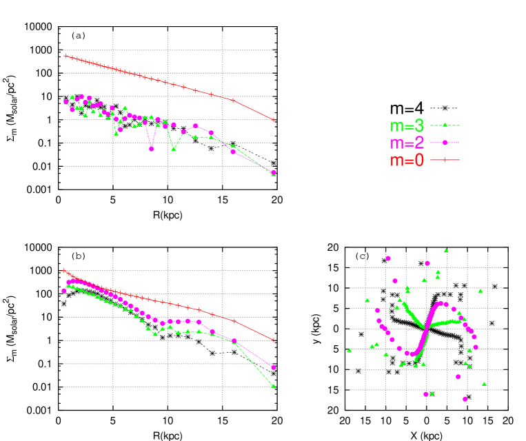
Figure 7: Modal analysis of the disk surface density profile for th model S. The notations are the same as Fig. 6, but the panel (b) and (c) are at $T=1.4$ Gyr.

Figures 6 and 7 show the surface density modes for the model L and S, respectively. The panel (a) shows the coefficient $\Sigma_{m}(R)$ at the initial time. Each annulus contains 16,384 particles. The $m=0$ profiles show the exponential distribution of the disk surface density. The higher modes exist only as noises at the beginning. After about 1 Gyr (panel (b) and (c)) the profiles show that a bar formed at the center. The bar in the model S is strong and large, while that in the model L is 2 or 3 times smaller than in the model S. The formation of a bar is expected for models with smaller bulges [ostr1973, sell2001]. We would take the realistic value for the bulge mass rather than take a larger bulge to prevent the bar instability. In fact, the Milky Way does have a bar. Therefore our models correctly reflect the same dynamics as the real Milky Way.

Disk vertical displacement within a annulus $R^{(k-1)}<R<R^{(k)}$ can be also expanded in a Fourier series;

$$z_{\mathrm{warp}}^{(k)}(\phi)=\sum_{m}h_{m}^{(k)}\cos(m|\phi-\psi_{m}^{(k)}|)=\sum_{m}\left[a_{m}^{(k)}\cos(m\phi)+b_{m}^{(k)}\sin(m\phi)\right].$$ (22)

A way to determine the coefficients is least squares fitting, in which the square deviation,

$$\left(\delta^{(k)}\right)^{2}\equiv\langle(z_{i}-z_{\mathrm{warp}}(\phi_{i}))^{2}\rangle\equiv\sum_{R^{(k-1)}<R_{i}<R^{(k)}}\frac{m_{i}}{\Delta S^{(k)}\overline{\Sigma}^{(k)}(\phi_{i})}(z_{i}-z_{\mathrm{warp}}(\phi_{i}))^{2}$$ (23)

becomes the minimum. In this expression, the average, $\langle\dots\rangle$, is normalized by the local surface density in order to avoid virtual warping modes owing to the bar or spiral arms. For the sake of simplicity, we will omit the suffix ^(k) from now on. The conditions which minimize $\delta^{2}$ are

$$\frac{\partial\delta^{2}}{\partial a_{0}} = 2\sum_{m^{\prime}}\left[a_{m^{\prime}}\langle\cos(m^{\prime}\phi_{i})\rangle+b_{m^{\prime}}\langle\sin(m^{\prime}\phi_{i})\rangle\right]-2\langle z_{i}\rangle=0,$$ (24)

$$\frac{\partial\delta^{2}}{\partial a_{m}} = 2\sum_{m^{\prime}}\left[a_{m^{\prime}}\langle\cos(m\phi_{i})\cos(m^{\prime}\phi_{i})\rangle+b_{m^{\prime}}\langle\cos(m\phi_{i})\sin(m^{\prime}\phi_{i})\rangle\right]-2\langle z_{i}\cos(m\phi_{i})\rangle$$ (25)

$$= 0,$$

$$\frac{\partial\delta^{2}}{\partial b_{m}} = 2\sum_{m^{\prime}}\left[a_{m^{\prime}}\langle\sin(m\phi_{i})\cos(m^{\prime}\phi_{i})\rangle+b_{m^{\prime}}\langle\sin(m\phi_{i})\sin(m^{\prime}\phi_{i})\rangle\right]-2\langle z_{i}\sin(m\phi_{i})\rangle$$ (26)

$$= 0.$$

In the analytical limit where $N$-body sampling is fairly well, the following relations stand

$$\langle\cos(m^{\prime}\phi_{i})\cos(m\phi_{i})\rangle = \left\{\begin{array}[]{ll}0&\mbox{for }m^{\prime}\neq m\\ \frac{1}{2}&\mbox{for }m^{\prime}=m\neq 0\\ 1&\mbox{for }m^{\prime}=m=0,\end{array}\right.$$ (30)

$$\langle\sin(m^{\prime}\phi_{i})\sin(m\phi_{i})\rangle = \left\{\begin{array}[]{ll}0&\mbox{for }m^{\prime}\neq m\\ \frac{1}{2}&\mbox{for }m^{\prime}=m,\end{array}\right.$$ (33)

$$\langle\sin(m^{\prime}\phi_{i})\cos(m\phi_{i})\rangle = 0.$$ (34)

If this is the case, the coefficients are determined by the following equations

$$a_{0} = \langle z_{i}\rangle,\quad a_{m}=2\langle z_{i}\cos(m\phi_{i})\rangle,\quad b_{m}=2\langle z_{i}\sin(m\phi_{i})\rangle$$ (35)

$$\delta^{2} = \left\langle\left(z_{i}-\sum(a_{m}\cos(m\phi)+b_{m}\sin(m\phi))\right)^{2}\right\rangle$$ (36)

$$= \langle z_{i}^{2}\rangle-a_{0}^{2}-\frac{1}{2}\sum\left(a_{m}^{2}+b_{m}^{2}\right).$$

Here $\delta$ is considered as the disk thickness, which is corrected by subtracting the effect of warping.

In practical calculations, however, finite $N$-body sampling causes errors in eqs. (30) – (34), the least mean square conditions eqs. (24) – (26) become thus a matrix equation. In order to estimate the errors owing to the coarse sampling, we also find another form of approximate solutions, in which the higher order coefficients are progressively determined by the lower order terms.

$$a_{0}=\frac{\langle z_{i}\rangle}{\langle 1\rangle},$$ (37)

$$a_{1}=\frac{\langle z_{i}\cos(\phi_{i})\rangle-a_{0}\langle\cos(\phi_{i})\rangle}{\langle\cos^{2}(\phi_{i})\rangle},\quad b_{1}=\frac{\langle z_{i}\sin(\phi_{i})\rangle-a_{0}\langle\sin(\phi_{i})\rangle}{\langle\sin^{2}(\phi_{i})\rangle},$$ (38)

$$a_{m}=\frac{\displaystyle\langle z_{i}\cos(m\phi_{i})\rangle-\sum_{m^{\prime}=0}^{m-1}\left[a_{m^{\prime}}\langle\cos(m\phi_{i})\cos(m^{\prime}\phi_{i})\rangle+b_{m^{\prime}}\langle\cos(m\phi_{i})\sin(m^{\prime}\phi_{i})\rangle\right]}{\langle\cos^{2}(m\phi_{i})\rangle},$$ (39)

$$b_{m}=\frac{\langle z_{i}\sin(m\phi_{i})\rangle-\displaystyle\sum_{m^{\prime}=0}^{m-1}\left[a_{m^{\prime}}\langle\sin(m\phi_{i})\cos(m^{\prime}\phi_{i})\rangle+b_{m^{\prime}}\langle\sin(m\phi_{i})\sin(m^{\prime}\phi_{i})\rangle\right]}{\langle\sin^{2}(m\phi_{i})\rangle}.$$ (40)

Differences between eq. (35) and eqs. (37) – (40) are considered as errors.

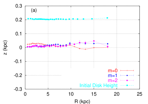
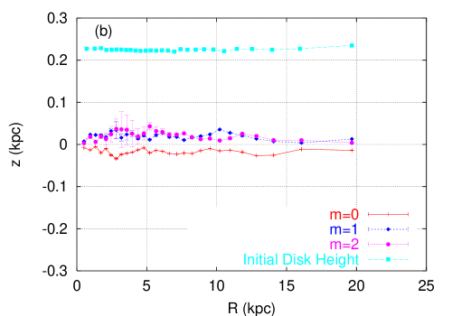
Figure 8: Amplitudes of the warping modes of the disk in the model L (panel a) and the model S (panel b), at $T=1.2$ Gyr and 1.4 Gyr, respectively. The modes $m=0$, 1, 2 are shown by the curves with plus (+), diamond ($\diamond$), and circle ($\circ{}$) symbols, respectively, and the initial disk thickness is shown by a curve with box ($\square$) symbols. The error bars denote difference between the solutions by eq. (35) and eqs. (37) – (40).

Figure 8 shows the amplitudes of the warping mode, $h_{m}(R)\equiv\sqrt{a_{m}^{2}(R)+b_{m}^{2}(R)}$, for $m=0$, 1, 2, after about 1 Gyr evolution without a satellite. The errors are shown by the error bars. Large errors occur at $R\sim 3$ kpc in the model S, where the strong bar appears. In other regions the errors are considerably smaller, and then invisible in the figures in those scales.

These warping modes are excited only by discreteness noises. W1998 suggested that the numerical noises could raise a large warp, if the number of particle in the system is less than 1,000,000. Comparing with the initial disk heights shown with light blue curves, it is obvious that the model galaxy disks are kept sufficiently flat over 1 Gyr.

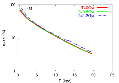
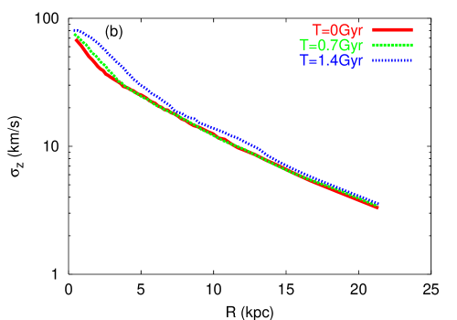
Figure 9: Change in the velocity dispersion in $z$-direction. The panel (a) and (b) show vertical velocity dispersion to the disk plane ($\sigma_{z}$) in the model L and S, respectively.

Two-body relaxation within the disk, and also random noise owing to the discrete distribution of halo material cause heating of the disk. This effect is estimated by change in velocity dispersions of the disk particles. Fig. 9 shows the evolution of $\sigma_{z}(R)$, which is evaluated in the same annuli as in the warp modal analysis for the model L and S. In both models, $\sigma_{z}$ increases significantly in the central part. This is explained by the disturbance from the bulge. In particular in the model S, the formation of the strong bar and its rotating motion might heat up the disk distribution. Except for the central part ($<5$ kpc), the increase in $\sigma_{z}$ is about 10% (or 1% in terms of energy increase), after about 1 Gyr evolution. In the main simulation we will follow the evolution six times longer, but expected heating would be still harmless.

From these analysis we are convinced that our Galaxy models are stable enough to discriminate the disk dynamics due to an orbiting satellite.

4.2 Satellite sinking and dynamical friction

The halo distribution is represented by truncated SCF basis-set. The necessary number of terms is determined by the requirement that the response of the halo to the satellite motion should be correctly solved. In this subsection we examine the nature of the SCF with respect to the number of terms included in the basis-set expansion.

We put the LMC model with a mass of $1.1\times 10^{10}M_{\odot}$, initially in a circular orbit with a radius $R=64$ kpc in the symmetry plane of the model L, but the bulge and disk component are replaced by a fixed external field. Only the halo component is solved by the SCF method. The changes in radius according to the satellite sinking are shown in Fig. 10.

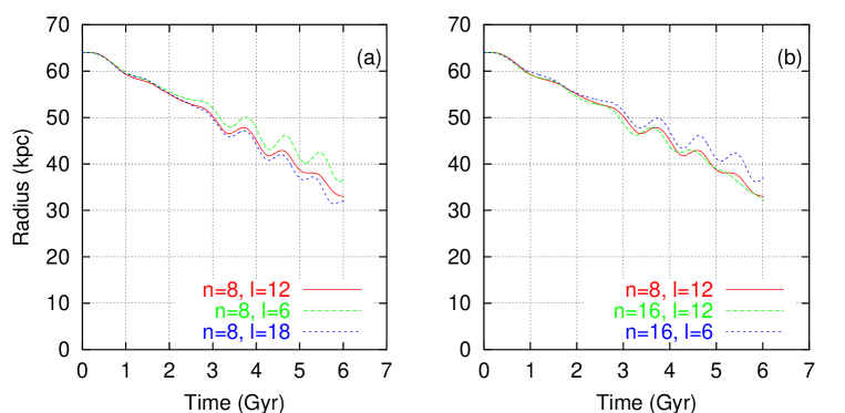
Figure 10: Evolution of the satellite’s orbits calculated with different SCF parameters. Each parameter of $n$ and $l$ means that the terms up to that value of $n$ and $l$ are included in the expansion of the basis set.

I have made six different runs with different number of terms in the expansion. As we have seen in Fig. 5, truncation of the radial expansion terms at $n=8$ or 9 yields a very good fit to the unperturbed halo distribution. On the other hand, the dynamical friction acting on the satellite should be more sensitive to the number of the azimuthal expansion terms. Fig. 10 (a) shows the satellite’s radius evolution calculated with different $l$ of the spherical harmonics. All the three runs are made with the radial expansion terms up to $n=8$, but the spherical harmonics are included up to $l=6$, 12, and 18. For each $l$, the parameter $m$ runs from $-l$ to $l$. In the run with $l=6$ the satellite sinking rate is slower than those with larger $l$. This is because contribution of terms with higher $l$ to dynamical friction is missing. Increasing $l$ from 12 to 18 makes the sinking rate faster, but the difference is not so large in comparison with the run with $l=6$. From the figure it is surmised that dynamical friction with $l=12$ is not far from the true value. The number of the spherical harmonics up to $l=12$ is the best compromise between accuracy of the dynamical friction and economy of the computational time.

In Fig. 10 (b) another comparison regarding the effect of the radial expansion number $n$ is shown. We find that including terms larger than $n=8$ does not change dynamical friction so much. Furthermore, we can make sure that number of the azimuthal expansion terms is the most important for dynamical friction because the run with $n=16$ but $l=6$ exhibits still smaller sinking rate.

4.3 Warp excitation

Finally we make simulations of the fully live Milky Way models interacting with the LMC model. Now the satellite is put in the realistic orbit described in section 2. The satellite is sinking in the halo owing to dynamical friction. The time variations in the distance of the LMC from the center of the Milky Way in the model L and S are shown in Fig. 11. In both models, the LMC is at a pericenter closer than 40 kpc near 6 Gyr. In fact, the pericenter at 40 kpc is smaller than that of the real LMC. This choice of the orbit makes the gravitational tide a little bit stronger in our model simulation. We would consider that the moment of 6 Gyr corresponds to the present day status. One might notice that in the model L the LMC sinks regularly, whereas it does not in the model S. Since the halo in the model S has the tidal cut off at 262 kpc, the satellite is on the edge of the halo distribution. This is because the halo in the model S has the tidal cut off around the orbit of the LMC.

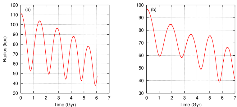
Figure 11: Change in the radius of the satellite in the model L (a) and the model S (b).

Time variation in the disk warping modes in the model L are shown in Fig. 12. Three rows (a), (b), and (c) correspond to the time $T=$ 0, 3.0, and 6.0 Gyr. In each row, the left panel shows the amplitudes of the warping mode with $m\leq 3$, together with the disk thickness. The right panel shows the position angle of the peak of the warping modes for each annuli in the disk plane. The diamond (blue) and round (pink) symbols denote $m=1$ and 2 modes, respectively. The disk rotation is clockwise in the figures. The LMC orbital plane intersects the disk nearly along the $y$-axis in the right panel. The first two intersections of the LMC with the initial disk plane are at ($X$, $Y$)=(6.8, -91.8) kpc and (-6.8, 89.3) kpc. At the beginning (panel a) all the warp modes are only due to noise, and thus the position angles are randomly distributed.

The observed warp amplitudes are also shown in the left panels for comparison. For the Milky Way, not only the $m=1$ but also $m=0$ and 2 modes are known to exist. We take an approximated formula for the warp amplitude given by binn1998, with a correction for the solar radius $R_{0}=8$ kpc,

$$z_{\mathrm{warp,obs}}(R,\phi)=\frac{R/\mathrm{kpc}-10.4}{5.6}\sin\phi+0.3\left(\frac{R/\mathrm{kpc}-10.4}{5.6}\right)^{2}(1-\cos 2\phi).$$ (41)

In Fig. 12 and 13 the observed $m=1$ and 2 modes are shown by dashed and dotted curves, respectively.

At 3 Gyr (panel b) disk warping appears in several modes. The most noticeable mode is $m=0$ (red solid line with “$+$” symbol). It has a wavy figure with the amplitudes about 250 pc upward and 400 pc downward. All the other modes have simple shapes with nearly same amplitudes. The amplitudes grow outwards, but the biggest amplitudes are still less than 500 pc. The $m=1$ mode shows a clear bending in the amplitude at around $R=10$ kpc, and the peaks of the $m=1$ mode make a broad ridge, which slightly winds towards the same direction as the disk rotation. The $m=2$ global bending mode is clearer in the position angle diagram which starts at 5 kpc, and winds in trailing sense. But outside of 11 kpc the mode becomes dispersed again, and shows no coherent feature.

At 6 Gyr (Panel c), which is considered as the present state, the amplitudes of the $m=0$ and 1 modes become larger. The largest amplitude of the $m=0$ is about 1 kpc. A bend in the $m=1$ curve appears at $R=7.5$ kpc, growing outwards up to the largest amplitude of 1 kpc. The ridge of the $m=1$ mode winds in trailing sense until 15 kpc, then turns to leading sense. Similar winding feature appears in the $m=2$ mode, which starts at 10 kpc, winds in trailing sense until 10 kpc, then starts winding oppositely. Since the LMC is revolving retrograde to the disk rotation, I surmise that warping modes are affected by the trailing wakes of the LMC (see Fig. 15 to Fig. 17), and that is the reason of the change of the trend in winding of the warping modes.

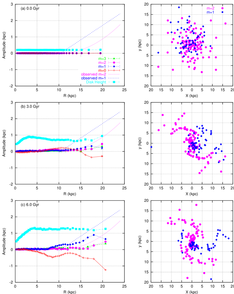
Figure 12: Warp modes in the model L. The rows (a), (b), (c) correspond to the time $T=$ 0, 3.0, and 6.0 Gyr, respectively. In each row, the left panel shows the amplitudes of the warping mode, and the right panel shows the position angle of the peak of the warping modes in the disk plane. The disk rotation is clockwise in the figures. The LMC orbital plane intersects the disk nearly along the $y$-axis in the right panel. The amplitude for uniform tilting of the disk is already subtracted from $m=1$ amplitudes in these figures.

The most remarkable result is that the warp amplitudes we have got from the simulation are already comparable to the observed ones. For the $m=0$ mode the amplitude is nearly the same amplitude as the observed one, though the sign is opposite. This negative amplitude in the $m=0$ might depend on the initial position of the LMC, which we took arbitrary in the present orbital plane. The $m=1$ and $m=2$ modes have more than a half of the observed amplitudes. The observed trend that the $m=2$ mode has about a half amplitude of the $m=1$ mode is also realized in the simulation. This result proves that in cooperation with the halo response the LMC can create enough tide to excite observable warps.

It should be noted that the disk plane is getting inclined homogeneously with respect to the initial disk plane. The tilting angles of inner part of the disk are about 3 degrees at $T=3$ Gyr, and 6 degrees at $T=6$  Gyr. Since the homogeneous tilting is not observed as a warp, these tilts are already subtracted from the $m=1$ mode. In fact, tilting itself can be the cause of warp [spar1988] if a halo is flattened. Our halo models are, however, spherical, so that tilting cannot develop the integral-shaped warps.

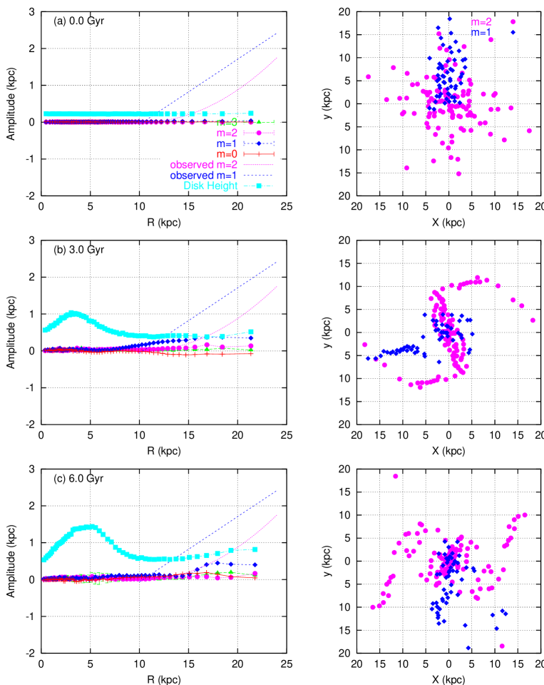
Figure 13: Warp modes in the model S. Notations in this figure are the same as Fig. 12. The error bars seen in the left panel (c) are the errors in the surface density correction on the estimate of warp modes, which is explained in section 4.1.

Fig. 13 shows the warping modes in the model S. The notations are the same as those in Fig. 12. At $T=3$ Gyr (panel b), a coherent $m=1$ bending mode (dashed curve with filled diamond symbol) is developed. The bend starts at 8 kpc, and the ridge of the $m=1$ warp makes a straight line. This feature resembles the observed warp very well, but its amplitude is at largest 400 pc. This is significantly smaller than the observed warp. The other modes are much smaller than the $m=1$ mode. At $T=6$ Gyr (panel c), all the warping modes still have small amplitudes, thus the development of warps seems already saturated. In the $m=1$ warping mode there is a step in the amplitudes at 15 kpc. Within this radius the peak position angles align in a straight line, but outside of the radius, the peak position angles wind and folded. This might be also due to the dominant effect of the wakes in the halo.

One thing that is clear by comparing the results of the two models is the importance of the halo distribution for excitation of warps. Both models have the same halo density at the solar radius, but the halo in the model S has a smaller cut off radius, hence the halo in the model S has smaller densities in the region where the LMC is orbiting. The wakes excited in the model S are thus smaller than those in the model L.

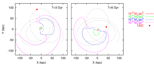
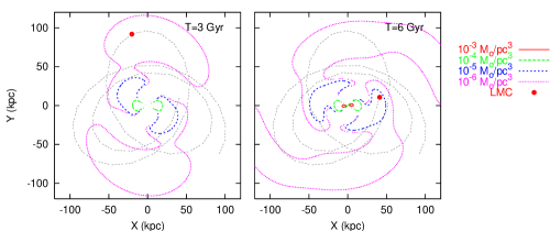
Figure 14: Density contour of the $m=1$ wake in the model L, in the section of the orbital plane of the LMC. The position of the LMC is denoted by a big dot, where its trajectory is shown by the dashed curve. The levels of the contours are shown in logarithmic density scales only for positive density enhancement.

Figure 15: Density contour of the $m=2$ wake in the model L. Notation is the same as Fig. 15. The enhancements that align to the horizontal axes in the central region with $R<20$ kpc are contribution from the disks.

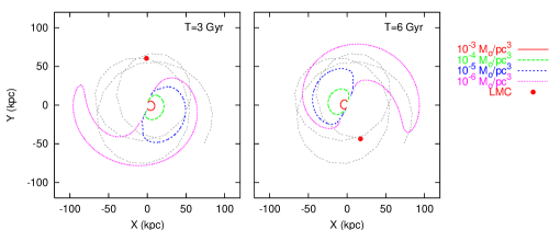
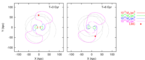
Figure 16: Density contour of the $m=1$ wake in the model S. Notation is the same as Fig. 15.

Figure 17: Density contour of the $m=2$ wake in the model S. Notation is the same as Fig. 15. The enhancements that align to the horizontal axes in the central region with $R<20$ kpc are contribution from the disks.

Figs. 15 to 17 show contour maps of the $m=1$ and 2 wakes in the section of the halo cut by the orbital plane of the LMC. In the figures the disks are nearly edge on with the inclination of 80 degrees, and the section of the disk planes are aligned to the horizontal axes. The wakes are defined as spherical harmonic components of the halo density. Only positive density regions are plotted. The position of the LMC is shown by a large dot, and its trajectory to 6 Gyr is superposed with a dashed curve. In this plane the LMC revolves anti-clockwise.

One should note that the amplitude of the $m=1$ mode has uncertainty depending on the selection of the origin of expansion. Even for the spherical distribution, deviation of the origin from the center of the distribution yield virtual $m=1$ mode. For example, the deviation of the origin of 625 pc causes a $m=1$ mode with amplitude of $10^{-5}M_{\odot}\mathrm{pc}^{-3}$ at $r=50$ kpc, which is comparable to the one shown in Fig. 15. Our choice of the origin of expansion is the center of mass of the most tightly bound particles, which is determined in the same way as the SCF expansion. With this choice of the origin, the error in the determination of the origin of expansion cannot be larger than the size of the core ($\sim 500$ pc), so that the errors in the amplitude of the wake are much smaller than the amplitude of the wake.

The innermost density enhancements with a size of 20 kpc, which are seen in the $m=2$ plots (Fig. 15 and 17), are contributions from the disk. These figures show that large scale wakes are excited nearly at the radius of the LMC. It is clear that the wakes in the model L are larger and stronger than those in the model S. In particular for the $m=2$ wakes, which would be the direct cause of the integral-shaped warps, two crescent-shaped wakes are seen in Fig. 15. One is an outer pair with a radius of 70 kpc, which typically appears in the $10^{-6}M_{\odot}/\mathrm{pc}^{3}$ contours, and the other is an inner pair with a radius of 30 kpc, which are seen as the contours of $10^{-5}M_{\odot}/\mathrm{pc}^{3}$. Those should correspond to the wakes which have resonant rotational frequencies 1:1 and 2:1 to that of the LMC. This is exactly the same feature as those obtained in Weinberg’s analysis. In the model S (Fig. 17), however, no clear inner wake can be seen other than the disk contribution. This might be because the halo density is too small and the disk gravity is still dominating in the region.

5 Conclusion and Discussions

Our study is meant to be an extension of Weinberg’s linear analysis [wein1998c], in the way that (i) the simulations are made by a fully-selfconsistent $N$-body code, (ii) the disk is three-dimensional, and (iii) the Galaxy models are more realistic. The warp amplitude that we have got in the model L is nearly the same as that of the largest warp in W1998. An interesting difference between our results and W1998 is that our smaller halo mass model yields smaller warp amplitudes, while in W1998 larger halo models yield smaller warps. This is, in fact, explainable as follows. In W1998, different halo masses produce different rotation curves, so that larger halo mass models reduce the efficiency of resonant amplification of warps. In our case the masses of the disk, bulge and halo within $R=50$ kpc are nearly the same between the models, hence the rotation curves in smaller scales are also the same. Therefore the resonant structures are not very different between the models. On the other hand, the mass within $R=170$ kpc is twice as massive in the model L as that in the model S. In fact the warp amplitude in the model L is roughly double of the model S. This linear dependence shows that the mass of a halo in the region where a satellite is orbiting has a direct effect on warp amplitudes. As a result we confirmed W1998’s prediction that halos play crucial role in warp excitation.

Our high resolution simulations upon the Galaxy models with reasonably realistic parameters make it possible to compare the numerical results with the observations seriously. Our larger halo model yields very large warp, which is comparable to the observed warp. The $m=0$ harmonic mode has nearly the same amplitude as the observed one, while those of $m=1$ and 2 are about a half. These values are in fact remarkably close to those of the observed warp. Now the LMC has revived as a possible candidate for the main cause of the Galactic warp. Though there are still problems, e.g., the lines of nodes are not straight, we have resolved the most serious problem of the interaction scenario, that the gravitational tide from the LMC would be too small to excite the observed warp.

In this paper, we examined the LMC as a main contributer to the Galactic warp. On the other hand, the Sgr dwarf was posed as another candidate. Though its current mass is much smaller ($\sim 10^{9}M_{\odot}$) than the LMC, its position is closer (20 kpc), thus the gravitational tide is comparable to that of the LMC. jian2000 proposed a possibility that the Sgr dwarf had $\sim 10^{11}M_{\odot}$ initially. Moreover, since the orbital plane of the Sgr dwarf is perpendicular to that of the LMC, the induce warp would have a line of nodes perpendicular to that induced by the LMC. Therefore examination of different satellite parameters is certainly important to find out the origin of the Galactic warp.

We have also found that our smaller halo model cannot bear the observed warp. This result shows that even in the interaction scenario the halos play an important role, so that we could use the warp kinematics as a probe of the halo structure. Our results might suggest that a massive halo is necessary to excite the observed Galactic halo if its origin is the LMC. In order to restrict halo properties, however, we need to explore wider model parameters. We could change the contribution of the halo material within the disk radius smaller to examine the maximal disk models. While mera1998b argued that a maximal disk model is excluded, a possibility that the Milky Way has a maximal disk is shown in several papers[sack1997, palu2000, binn2001b]. Moreover the strongest warp appeared in the maximal disk model in W1998, which motivated us to investigate the maximal disk models. Another possible extension of model parameters is the halo flattening. Our selection of the spherical halo ($q=1.0$) is based on the analysis of ibat2001, but other analysis shows that the most probable flatness of the halo is $c/a=0.8$ [olli2000]. As mentioned in Sect. 4.3 the disk in the model L is getting inclined to not negligible extent, so that if the halo is flattened the tilting disks would get additional torque from the halo, which might make the warp amplitude larger. Since the shape of the halo is still under big arguments, for example, studies of galaxy formation by means of cosmological simulations conclude that the galactic halos are much more flattened such as $c/a\sim 0.5$ [warr1992, dubi1994]. Not only the shape but also the different velocity distribution in the halo may affect the warp amplitude, because the wake structure might be different. We will tackle these problems in detail in subsequent papers.

There is another interesting outcome from our simulations besides the warp. Quite large disk heating has taken place especially in the model L. Even though we cannot exclude the artifical heating effect in numerical schemes, since such a large heating is not observed in the test simulation without a satellite. We surmise that interaction with a satellite also causes disk heating. The same heating owing to interaction with a satellite was studied by vela1999, who claimed that satellites on prograde orbits causes disk heating more than those on retrograde orbits. Our simulations results larger heating than vela1999. This is partly because our initial disks are about three times thinner than those in vela1999. Since the disk heating is, as mentioned in Sect. 3.1, a very delicate problem for all numerical methods, we need much more careful treatment for this problem. This will be our next project.

Appendix A Input parameters for the Galaxy model construction

For construction of the initial Galaxy models, I have used the software ‘GalactICS’ [kuij1995]. This software is available on their web site (http://www.astro.rug.nl/{̃}kuijken/galactics.html). The software requires several input parameters. Here is the list of the input parameters. The parameters explained in Sec. 2 are listed in the column 1, and the corresponding variables used in the codes are listed in the column 2. The column 3 and 4 are the values of the parameters for the model L and S, respectively. All the values are in the computational units, where the gravitational constant, the mass of the disk, and the scale length of the disk are set to unity.

Table 2: Input parameters given to the software GalactICS.

		model L	model S
halo
cental potential $\Psi_{0}$	psi00	$-5.0$	$-4.0$
velocity scale $\sigma_{0}$	v0	0.90	1.0
potential flattening $q$	q	1.0	1.0
core parameter $R_{\mathrm{c}}^{2}/R_{\mathrm{K}}^{2}$ ∗1	coreparam	0.1	0.1
characteristic halo radius $R_{\mathrm{a}}$ ∗2	ra	0.7	0.8
disk
disk mass $M_{\mathrm{d}}$	rmdisk	1.0	1.0
scale length $R_{\mathrm{d}}$	rdisk	1.0	1.0
disk radius $R_{\mathrm{out}}$	outdisk	7.0	7.0
scale height $z_{\mathrm{d}}$	zdisk	0.07	0.07
truncation width $\delta R$	drtrunc	0.5	0.5
central radial vel. dispersion, $\sigma_{R}(0)$	sigr0	0.55	0.55
scale length of $\sigma_{R}^{2}$	disksr	1.0	1.0
bulge
central density $\rho_{\mathrm{b}}$	rho1	15.0	15.0
cutoff potential $\Psi_{\mathrm{c}}$	psiout	$-4.12$	$-3.1$
velocity dispersion $\sigma_{\mathrm{b}}$	sigbulge	0.8	0.8
radial step size	dr	0.01	0.01
number of bins	nr	51000	10000
Maximum azimuthal harmonic	lmax	10	10

($\ast$1) $R_{\mathtt{K}}$ is the King radius

($\ast$2) Characteristic radius is related to the density scale $\rho_{1}$ by the following relation; $R_{\mathrm{a}}\equiv[3/2\pi G\rho_{1}]^{1/2}\sigma_{0}\mathrm{e}^{\Psi_{0}/2\sigma_{0}^{2}}$

References

- [1] \harvarditemAlves \harvardand Nelson2000alve2000 Alves, D.R., Nelson, C.A., 2000 ApJ, 542, 789. (2000ApJ...542..789A)
- [2] \harvarditemBarnes \harvardand Hut1986barn1986 Barnes, J., Hut, P., 1986, Nature, 324, 446. (1986Natur.324..446B)
- [3] \harvarditemBinney \harvardand Tremaine1987binn1987 Binney, J., Tremaine, S., 1987, Galactic dynamics, Princeton University Press, Princeton. (1987gady.book.....B)
- [4] \harvarditemBinney1992binn1992 Binney, J., 1992, ARAA, 30, 51. (1992ARA&A..30...51B)
- [5] \harvarditemBinney \harvardand Merrifield1998binn1998 Binney, J., Merrifield, M., 1998, Galactic Astronomy, Princeton University Press, Princeton. (1998gaas.book.....B)
- [6] \harvarditemBinney et al.1998binn1998a Binney, J., Jiang, I.G., Dutta, S., 1998, MNRAS, 297, 1237. (1998MNRAS.297.1237B)
- [7] \harvarditemBinney \harvardand Evans2001binn2001b Binney, J., Evans, N.W., 2001, MNRAS, 327, L27. (2001MNRAS.327L..27B)
- [8] \harvarditemBosma1991bosm1991 Bosma, A., 1991, in: S. Casertano, P. Sackett, F. Briggs (eds.) Warped Disks and Inclined Rings around Galaxies, Cambridge University Press Cambridge. (1991wdir.conf..181B)
- [9] \harvarditemBriggs1990brig1990 Briggs, F.H., 1990, ApJ, 352, 15. (1990ApJ...352...15B)
- [10] \harvarditemBurke1957burke1957 Burke, B.F., 1957, AJ, 62, 90. (1957AJ.....62...90B)
- [11] \harvarditemChandrasekhar1943chan1943 Chandrasekhar, S., 1943, ApJ, 97, 255. (1943ApJ....97..255C)
- [12] \harvarditemClutton-Brock1973clut1973 Clutton-Brock, M., 1973, APSS, 23, 55. (1973Ap&SS..21...79C)
- [13] \harvarditemDehnen \harvardand Binney1998dehn1998c Dehnen, W., Binney, J.J., 1998, MNRAS, 298, 387. (1998MNRAS.298..387D)
- [14] \harvarditemDiplas \harvardand Savage1991dipl1991 Diplas, A. Savage, B.D., 1991, ApJ, 377, 126. (1991ApJ...377..126D)
- [15] \harvarditemDubinski1994dubi1994 Dubinski, J., 1994, ApJ, 431, 617. (1994ApJ...431..617D)
- [16] \harvarditemDubinski \harvardand Kuijken1995dubi1995 Dubinski, J., Kuijken, K., 1995, ApJ, 442, 492. (1995ApJ...442..492D)
- [17] \harvarditemEarn1996earn1996 Earn, D.J.D., 1996, ApJ, 465, 91. (1996ApJ...465...91E)
- [18] \harvarditemHenderson et al.1982hend1982 Henderson, A.P., Jackson, P.D., Kerr, F.J., 1982, ApJ, 263, 116. (1982ApJ...263..116H)
- [19] \harvarditemHernquist1987hernq1987 Hernquist, L., 1987, ApJS, 64, 715. (1987ApJS...64..715H)
- [20] \harvarditemHernquist1990hernq1990a Hernquist, L., 1990, ApJ, 356, 359. (1990ApJ...356..359H)
- [21] \harvarditemHernquist \harvardand Ostriker1992hernq1992 Hernquist, L., Ostriker, J.P., 1992, ApJ, 386, 375. (1992ApJ...386..375H)
- [22] \harvarditemHofner \harvardand Sparke1994hofn1994 Hofner, P., Sparke, L.S., 1994, ApJ, 428, 466. (1994ApJ...428..466H)
- [23] \harvarditemHunter \harvardand Toomre1969hunt1969 Hunter, C., Toomre, A., 1969, ApJ, 155, 747. (1969ApJ...155..747H)
- [24] \harvarditemIbata et al.2001ibat2001 Ibata, R., Lewis, G.F., Irwin, M., Totten, E., Quinn, T., 2001, ApJ, 551, 294. (2001ApJ...551..294I)
- [25] \harvarditemIdeta et al.2000idet2000 Ideta, M., Hozumi, S., Tsuchiya, T., Takizawa, M., 2000, MNRAS, 311, 733. (2000MNRAS.331..733I)
- [26] \harvarditemJiang \harvardand Binney1999jian1999 Jiang, I.G., Binney, J., 1999, MNRAS, 303, L7. (1999MNRAS.303L...7J)
- [27] \harvarditemJiang \harvardand Binney2000jian2000 Jiang, I.G., Binney, J., 2000, MNRAS, 314, 468. (2000MNRAS.314..468J)
- [28] \harvarditemKerr1957kerr1957 Kerr, F.J., 1957, AJ, 62, 93. (1957AJ.....62...93K)
- [29] \harvarditemKroupa \harvardand Bastian1997krou1997a Kroupa, P., Bastian, U., 1997, NewA, 2, 77. (1997NewA....2...77K)
- [30] \harvarditemKuijken \harvardand Dubinski1995kuij1995 Kuijken, K., Dubinski, J., 1995, MNRAS, 277, 1341. (1995MNRAS.277.1341K)
- [31] \harvarditemKuijken \harvardand Gilmore1991kuij1991b Kuijken, K., Gilmore, G., 1991, ApJL, 367, L9. (1991ApJ...367L...9K)
- [32] \harvarditemMéra et al.1998mera1998b Méra, D., Chabrier, G., Schaeffer, R., 1998, AA, 330, 953. (1998A&A...330..953M)
- [33] \harvarditemMurai \harvardand Fujimoto1980mura1980 Murai, T., Fujimoto, M., 1980, PASJ, 32, 581. (1980PASJ...32..581M)
- [34] \harvarditemNelson \harvardand Tremaine1995nels1995 Nelson, R.W., Tremaine, S., 1995, MNRAS, 275, 897. (1995MNRAS.275..897N)
- [35] \harvarditemOlling \harvardand Merrifield2000olli2000 Olling, R.P., Merrifield, M.R., 2000, MNRAS, 311, 361. (2000MNRAS.331..361O)
- [36] \harvarditemOstriker \harvardand Binney1989ostriker-e1989 Ostriker, E.C., Binney, J.J., 1989, MNRAS, 237, 785. (1989MNRAS.237..785O)
- [37] \harvarditemOstriker \harvardand Peebles1973ostr1973 Ostriker, J.P., Peebles, P.J.E., 1973, ApJ, 186, 467. (1973ApJ...186..467O)
- [38] \harvarditemPalunas \harvardand Williams2000palu2000 Palunas, P., Williams, T.B., 2000, AJ, 120, 2884. (2000AJ....120.2884P)
- [39] \harvarditemPrendergast \harvardand Tomer1970pren1970 Prendergast, K.H., Tomer, E., 1970, AJ, 75, 674. (1970AJ.....75..674P)
- [40] \harvarditemReshetnikov \harvardand Combes1998resh1998 Reshetnikov, V., Combes, F., 1998, AA, 337, 9. (1998A&A...337....9R)
- [41] \harvarditemRobijn \harvardand Earn1996robi1996 Robijn, F.H.A., Earn, D.J.D., 1996, MNRAS, 282, 1129. (1996MNRAS.282.1129R)
- [42] \harvarditemSackett1997sack1997 Sackett, P.D., 1997, ApJ, 483, 103. (1997ApJ...483..103S)
- [43] \harvarditemSaha1993saha1993 Saha, P., 1993, MNRAS, 262, 1062. (1993MNRAS.262.1062S)
- [44] \harvarditemSánchez-Saavedra et al.1990sanc1990 Sánchez-Saavedra, M.L., Battaner, E., Florido, E., 1990, MNRAS, 246, 458. (1990MNRAS.246..458S)
- [45] \harvarditemSellwood \harvardand Evans2001sell2001 Sellwood, J.A., Evans, E.W., 2001, ApJ, 546, 176. (2001ApJ...546..176S)
- [46] \harvarditemShang et al.1998shan1998 Shang, Z., Zheng, Z., Brinks, E. et al., 1998, ApJL, 504, L23. (1998ApJ...504L..23S)
- [47] \harvarditemSparke \harvardand Casertano1988spar1988 Sparke, L.S., Casertano, S., 1988, MNRAS, 234, 873. (1988MNRAS.234..873S)
- [48] \harvarditemSyer1995syer1995 Syer, D., 1995, MNRAS, 276, 1009. (1995MNRAS.276.1009S)
- [49] \harvarditemTremaine \harvardand Weinberg1984trema1984 Tremaine, S., Weinberg, M.D., 1984, MNRAS, 209, 729. (1984MNRAS.209..729T)
- [50] \harvarditemVelázquez \harvardand White1999vela1999 Velázquez, H., White, S.D.M., 1999, MNRAS, 304, 254. (1999MNRAS.304..254V)
- [51] \harvarditemVine \harvardand Sigurdsson1998vine1998 Vine, S., Sigurdsson, S., 1998, MNRAS, 295, 475. (1998MNRAS.295..475V)
- [52] \harvarditemWarren et al.1992warr1992 Warren, M.S., Quinn, P.J., Salmon, J.K., Zurek, W.H., 1992, ApJ, 399, 405. (1992ApJ...399..405W)
- [53] \harvarditemWeinberg1998wein1998c Weinberg, M.D., 1998, MNRAS, 299, 499. (1998MNRAS.299..499W)
- [54] \harvarditemWilkinson \harvardand Evans1999wilk1999 Wilkinson, M.I., Evans, N.W., 1999, MNRAS, 310, 645. (1999MNRAS.310..645W)
- [55] \harvarditemZhao1996zhao1996 Zhao, H., 1996, MNRAS, 278, 488. (1996MNRAS.278..488Z)
- [56]