Neural networks and photometric redshifts

We present a neural network based approach to the determination of photometric redshift. The method was tested on the Sloan Digital Sky Survey Early Data Release (SDSS-EDR) reaching an accuracy comparable and, in some cases, better than SED template fitting techniques. Different neural networks architecture have been tested and the combination of a Multi Layer Perceptron with 1 hidden layer (22 neurons) operated in a Bayesian framework, with a Self Organizing Map used to estimate the accuracy of the results, turned out to be the most effective. In the best experiment, the implemented network reached an accuracy of 0.020 (interquartile error) in the range $0<z_{phot}<0.3$, and of 0.022 in the range $0<z_{phot}<0.5$.

1 Introduction

Ongoing and planned digital surveys such as the Sloan Digital Sky Survey and the implementation of an International Virtual Observatory, will enormously increase the quality and the amount of data available to the astronomical community. The scientific exploitation of these data, while promising new answers to old questions, is also stimulating the implementation of new tools capable to deal in an effective way with unprecedently large volumes of data. One field which will be deeply affected by these new data sets is that of the large scale of the universe. Planned or ongoing surveys such as the Sloan Digital Sky Survey (SDSS,;York et al. 2000), the VIRMOS-VLT Survey (Le Fèvre et al. 2000), the VST Survey (G. Busarello, private communication) will provide a huge amount of high accuracy spectroscopic and photometric data which will enable observational cosmologists to map with unprecedented accuracy and detail the properties and the structure of the Universe.

In this respect it needs to be stressed that, in spite of the recent and well known advances in multiobject spectroscopy, photometric redshifts (cf. Baum 1962, Pushell et al. 1982) derived from multicolor photometry have been for a long time and still are the only tool which may be effectively used to evaluate the distances of large number of galaxies. Most photometric redshifts methods rely on a $\chi^{2}$ fitting of a library of template Spectral Energy Distributions (hereafter SEDs) to the observed data points, and differ mainly in how the SEDs are derived and on how they are fitted to the data.

SEDs may either be derived from population synthesis models (cf. Bruzual and Charlot 1993) or be spectra of real objects selected in order to ensure a sufficient coverage of morphological types and/or luminosity classes. As effectively stressed by Koo (1999), both approaches (synthetic and empirical) have their pro’s and con’s.

Synthetic spectra, for instance, sample an ’a priori’ defined grid of mixtures of stellar populations and may either include unrealistic combinations of parameters or exclude some unknown cases, while empirical templates are usually derived from nearby and bright galaxies and may therefore be not representative of the spectral properties of galaxies falling in other redshift ranges. The various methods are extensively compared and discussed in several papers (cf. Koo 1999; Fernandez-Soto et al. 2001) and have been applied to many different data sets such as the Hubble Deep Field (cf. Massarotti et al. 2001a, 2001b) .

Another approach, which is in the same line of the one discussed in this paper, can be applied only to what we shall call ’mixed surveys’, id est datasets where accurate and multiband photometric data for a large number of objects are supplemented by spectroscopic redshifts for a small but statistically significant subsample of the same objects. In this case, the spectroscopic data can be used to constrain the fit of a polynomial function mapping the photometric data (cf. Connolly et al. 1995, Wang et al. 1998, Brunner et al. 2000). It needs to be stressed that, at difference with the SED fitting methods, this interpolative approach cannot be effectively applied to objects fainter than the spectroscopic limit since, in absence of an ’a priori’ knowledge, impossible extrapolations would be required. It could be argued that the needed ’a priori’ knowledge could be extracted from population synthesis models, but it is apparent that, in this case, the uncertainties of the two methods would add up and SED’s fitting methods would - in any case - be more accurate and preferable.

Interpolative methods, however, offer the great advantage that they are trained on the real Universe and do not require strong assumptions on the physics of the formation and evolution of stellar populations. Neural Networks (hereafter NNs) are known to be excellent tools for interpolating data and for extracting patterns and trends (cf. the standard textbook by Bishop 1995) and in this paper, we shall discuss the application of a set of neural tools to the determination of photometric redshifts in large ”mixed surveys” (cf. Giordano 2001). In section 2 we introduce the basic concepts of Neural Networks paying special attention to the Multi Layer Perceptron and the Self Organising Maps; in Section 3 we discuss a first application to the SDSS Early Data Release data (Stoughton et al. 2001) and in Section 4 we show how SOM can be used to evaluate the degree of contamination of the final redshift catalogues. In Section 5, finally we shall draw our conclusions and discuss some possible applications of the neural tools. In a forthcoming paper we shall compare the results of different photometric redshifts methods applied to the same SDSS-EDR data and will discuss the properties of the photometric redshift catalogue derived with the method described in this paper (Longo et al. 2002, in preparation).

2 Neural Networks

NNs, over the years, have proven to be a very powerful tool capable to extract reliable information and patterns from large amounts of data even in the absence of models describing the data (cf. Bishop 1995) and are finding a wide range of applications also in the astronomical community: catalogue extraction (Andreon et al. 2001), star/galaxy classification (Bertin and Arnout, 1996, Andreon et al. 2001), galaxy morphology (Storrie-Lombardi et al. 1992; Lahav et al. 1996), classification of stellar spectra (Bailer and Jones 1998, Allende Prieto et al. 2000, Weaver 2000), data quality and data mining (Tagliaferri et al. 2002).

A NN is usually structured into an input layer of neurons, one or more ”hidden” layers and one output layer. Neurons belonging to adiacent layers are usually fully connected and the various types and architectures of the NNs are identified by the different topologies adopted for the connections and by the choice of the activation function (details can be found in the standard book by Bishop 1995). From the operational point of view, NNs can be divided into two main types, supervised and unsupervised systems, accordingly to the type of learning.

In the first case, NNs learn how to recognise a specific pattern or characteristic on a set (hereafter ”training set”) of labeled data containing for each input vector also the desired output (hereafter ”target”). In unsupervised systems, instead, NNs look for the statistical similarity of the imput data. In this work both types of NNs are used to perform different tasks.

The AstroMining software (Longo et al. 2001) is a package written in the MatLab ©  environment to perform a large number of data mining and knowledge discovery tasks, both supervised and unsupervised, in large multiparametric astronomical datasets. The package relies also on the Matlab ©  ”Neural Network”, the ”SOM” (Vesanto 1997) and the ”Netlab” (Nabney and Bishop 1998) toolboxes.

AstroMining accepts as input any ASCII table containing a header describing the contents of each colum and then a set of parameters. Via interactive interfaces, it is possible to perform a large number of operations: i) manipulation of the input data sets; ii) selection of relevant parameters; iii) selection of the type of neural architecture; iv) selection of the training validation and test sets construction procedure; v) etc. The package is completed by a large set of visualization and statistical tools which allow to estimate the reliability of the results and the performances of the network. The user friendliness and the generality of the package allow both a wide range of applications and the easy execution of experiments (more details on other aspects of the AstroMining tool which are not relevant to the present work may be found in Tagliaferri et al. 2002).

Let us focus now on some fundamental aspects connected with the use of supervised NNs. In order to perform correctly, almost all supervised NNs need to be trained, validated and tested on three independent datasets. In order to achieve good generalization performances, the training set needs to be representative of the typical data which will be passed to the network in the application phase. The validation data set (which is often and erroneously ignored in many NN applications) is a second dataset disjoined from the training set but having the same statistical properties. The role played by the validation set is subtle but crucial: by using the training set alone, in fact, the NNs (and the MLP in particular) may easily run into overfitting errors, thus loosing all generalization properties. It needs to be stressed in fact, that while the error computed on the training set may decrease asintotically, the capability of the network to reproduce patterns not encountered during the training phase may decrease (this is known as ’over-fitting’ condition), in other words, the NN will learn how to reproduce the patterns in the training set but will produce completely wrong results when applied to other data sets. The validation set prevents this from happening via a so called ’regularization technique’: during the training phase, at regular intervals, the training is interrupted (and the weights of the neurons are frozen), then the net is run on the validation set in order to compute the error with respect to the desired output; the training is stopped when the error computed on the validation set shows a significant increasing trend and, finally, the NN corresponding to the minimum error is selected.

After this phase the final performances of the resulting weight configuration are tested on a third data set, the so called ’test set’, which is, once more, completely disjoined from the previous two. Another regularization method not requiring a validation set, namely the Bayesian Learning Approach, will be described in the next paragraph.

2.1 The Multi Layer Perceptron - MLP

Due to its interpolation and capabilities, the Multi Layer Perceptron (MLP) is one of the most widely used neural architectures. As most other networks, the MLP is structured into an input layer, one or more hidden layers and one output layer (see figure 1). We implemented an MLP with one hidden layer and $n$ imput neurons, where $n$ is the number of parameters selected by the user as input in each experiment.

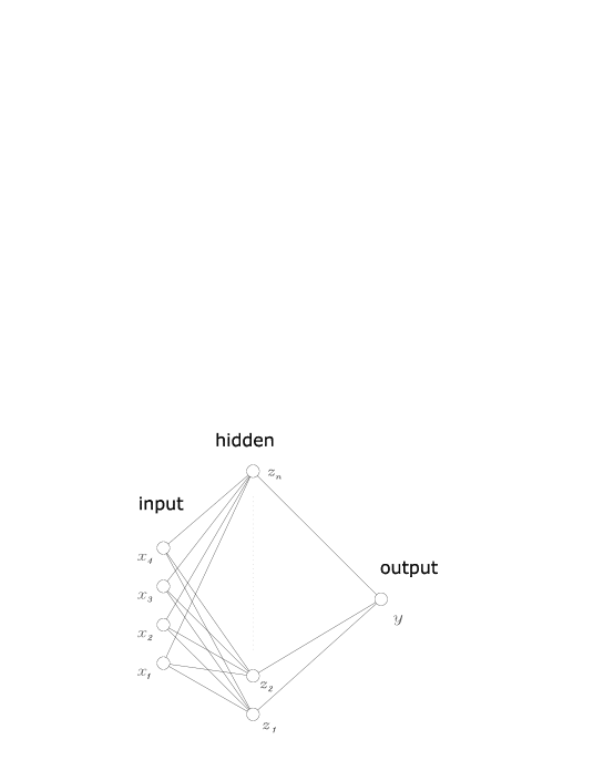
Figure 1: A schematic representation of the Multi Layer Perceptron

As just mentioned, it is also possible to train NN’s in a Bayesian framework, which allows to find the more efficient among a population of NN’s differing in the hyperparameters controlling the learning of the network (cf. Bishop 1995), in the number of hidden nodes, etc. The most important hyperparameters being the so called $\alpha$ and $\beta$. The parameter $\alpha$ is related to the weights of the network: a larger value for a component of $\alpha$ implying a less meaningful corresponding weight, thus allowing to estimate the relative importance of the different inputs (Automatic Relevance Determination; Bishop 1995) and, therefore, the selection of the input parameters which are more relevant to a given task. The parameter $\beta$ is instead related to the variance of the noise: a smaller value corresponding to a larger value of the noise and therefore to a lower reliability of the network. The Bayesian method allows the values of the regularization coefficients to be selected using only the training set, without the need for a validation set.

The implementation of a Bayesian framework requires several steps: initialization of weights and hyperparameters; training the network via a non linear optimization algorithm in order to minimize the total error function. Every few cycles of the algorithm, the hyperparameters are re-estimated and eventually the cycles are reiterated.

2.2 The Self Organizing Maps - SOM

The Self-Organizing Map (SOM), developed by Kohonen (1995), is one of the most used NN model. The SOM algorithm is based on unsupervised competitive learning, id est the training is entirely data-driven and all neurons of the map compete with each other producing only one winning neuron for each input vector. This property turns SOM into an ideal tool for KDD and expecially for its exploratory phase: data mining (Vesanto 1997). Among various other advantages, SOM allow an approximation of the probability density function of  the training data, the derivation of prototype vectors best describing the data, and a highly visualized and user friendly approach to the investigation of the data.

A SOM is composed by neurons located on a regular, usually 1 or 2-dimensional grid. Each neuron $i$ of the SOM is represented by an $n$-dimensional weight or reference

$m_{i}=\left[m_{i_{1}},m_{i_{2}},...,m_{i_{n}}\right]^{T}$

where $n$ is the dimension of the input vectors. Higher dimensional grids are not generally used since their visualization is much more problematic. Usually the map topology is a rectangle  but also toroidal topologies have been used successfully. The neurons of the map are connected to adjacent neurons by a neighborhood relation dictating the structure of the map. In the 2-dimensional case the neurons of the map can be arranged either on a rectangular or on a hexagonal lattice. The number of neurons determines the granularity of the resulting mapping, which affects the accuracy and the generalization capability of the SOM.

The use of SOM for data mining requires several steps : construction, normalization and initialization of the Data Set, (unsupervised) training, visualization of the resulting map, and, finally, analysis of the results. The first two steps depend on the individual data set to be processed and the normalization is made in order to achieve $mean=0$ and $variance=1$.

In the basic SOM algorithm, the topological relations and the number of neurons are fixed from the beginning. The number of neurons should usually be selected by trial and error, with the neighborhood size controlling the smoothness and generalization of the mapping. Before training, in the course of the initialization phase, initial values are given to the weight vectors. The SOM is robust regarding the initialization, but if properly accomplished it allows the algorithm to converge faster to a good solution. Typically, any of the following initialization procedures may be used:

• random initialization, with the weight vectors initialized with small random values;

• sample initialization, where the weight vectors are initialized with random samples drawn from the input data set;

• linear initialization, where the weight vectors are initialized in an orderly fashion along the linear subspace spanned by the two principal eigenvectors of the input data set. These eigenvectors can be calculated using Gram-Schmidt procedure (Kohonen 1995).

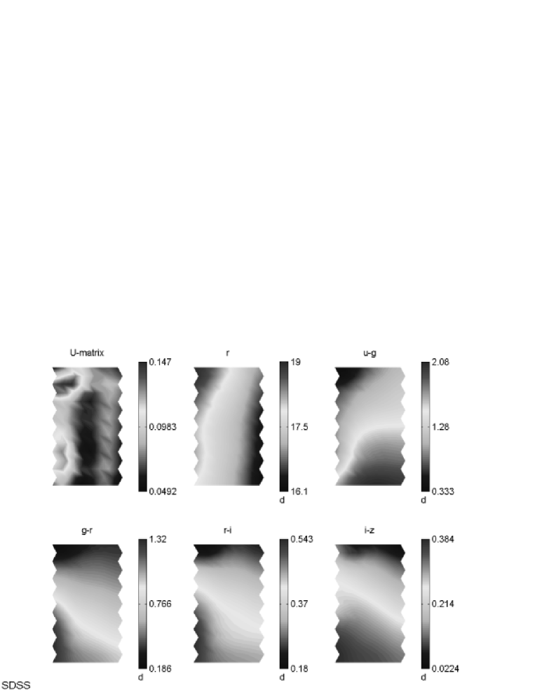
Figure 2: U matrix and plane components of a 120 nodes SOM applied to the SDSS-EDR data. The parameters are the r petrosian magnitude and the i-r, g-r, r-i, i-z colors. Regions of uniform color are the clusters. In spite of the rather uniform variation over the individual parameters, the U Matrix clearly shows the existence of several clusters. For an interpretation of the above, see Figure 5.

During the training phase, one sample vector $\mathbf{x}$ from the input data set is randomly chosen and a similarity measure is calculated between it and all the weight vectors of the map. The Best-Matching Unit (BMU), denoted as $c$, is the unit with weight vector having the greatest similarity with the input sample $\mathbf{x}$. The similarity is usually defined by means of a distance measure, typically an Euclidean distance. Formally the BMU is defined as the neuron for which:

$\left\|\mathbf{x}-\mathbf{m}_{c}\right\|={\min}_{i}\left\|\mathbf{x}-\mathbf{m}_{i}\right\|$

where $\left\|.\right\|$ denotes the distance measure.  After finding the BMU, the weight vectors of the SOM are updated. The weight vectors of the BMU and its topological neighbors are moved in the direction of the input vector, in the input space. The SOM update rule for the weight vector of the unit $i$ is:

$\mathbf{m}_{i}\left(t+1\right)=\mathbf{m}_{i}\left(t\right)+h_{ci}\left(t\right)\left[\mathbf{x}\left(t\right)-\mathbf{m}_{i}\left(t\right)\right]$

Where $t$ denotes the time, $\mathbf{x}(t)$ is the input vector and $h_{ci}(t)$ denotes the neighborhood kernel around the winner unit. The neighborhood kernel is a non-increasing function of time and of the distance of unit $i$ from the winner unit $c$. It defines the region of influence that the input sample has on the SOM. The kernel is composed by two parts: the neighborhood function $h(d,t)$ and the learning rate function $\alpha(t)$:

$h_{ci}\left(t\right)=h\left(\left\|\mathbf{r}_{c}-\mathbf{r}_{i}\right\|,t\right)\alpha(t)$

where $r_{i}$ is the location of unit $i$ on the map grid. The neighborhood function used in our experiments is the Gaussian neighborhood function:

$exp\left(\frac{-\left\|\mathbf{r}_{c}-\mathbf{r}_{i}\right\|^{2}}{2\sigma^{2}\left(t\right)}\right)$

The learning rate $\alpha(t)$ is a decreasing function of time. Two commonly used forms are a linear function and a function inversely proportional to time:

$\alpha(t)=\frac{A}{t+B}$

where $A$ and $B$ are some suitably selected constants. The training is usually performed into two phases. In the first phase, relatively large initial $\alpha$ value and neighborhood radius are used. In the second phase both the $\alpha$ value and the neighborhood are small from the beginning. This procedure corresponds to first tuning the SOM approximately to the same space as the input data and then fine-tuning the map. The SOM toolbox (Vesanto 1997) includes the tools for the visualization and analysis of SOM and, since the weight vectors are ordered on the grid, the visualization of the U matrix turns out to be expecially useful in the data understanding/survey phase. The U matrix visualizes the clustering structures of the SOM as distances (in the assumed metric) between neighboring map units, thus high values of the U-matrix indicate a cluster border, uniform areas of low values indicate clusters themselves.

In Figure 2, we show both the U matrix for the whole data set, and the structure of the individual components.

Another advantage of SOM is that it is relatively easy to label individual data, id est to identify which neuron is activated by a given input vector. The utility of these properties of the SOM will become clear in the next paragraphs.

3 Application to the SDSS-EDR data

A preliminary data release (Early Data Release or EDR) of the SDSS was made available to the public in 2001 (Stoughton et al. 2001). This data sets provides photometric, astrometric and morphological data for an estimated 16 millions of objects in two fields: an Equatorial $2^{circ}$ wide strip of constant declination centered around $\delta$=0 and a rectangular patch overlapping with the SIRTF First Look Survey.

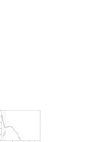
Figure 3: Logarithmic histogram of the redshifts in the SDSS-EDR. Notice the sharp discontinuity at z=0.5.

The EDR provides also spectroscopic redshifts for a little more than $50.000$ galaxies distributed over a large redshift range and is therefore representative of the type of the data which will be produced by the next generation of large scale surveys. In order to build the training, validation and test sets, we first extracted from the SDSS-EDR a set of parameters ($u$, $g$, $r$, $i$, $z$, both total and petrosian magnitudes, petrosian radii, $50\%$ and $90\%$ petrosian flux levels, surface brightness and extinction coefficients; Stoughton et al. 2001) for all galaxies in the spectroscopic sample.

In this data set, redshifts are distributed in a very dishomogeneous way over the range $0-7.0$ (Figure 3; $93\%$ of the objects have $z<0.7$).

Table 1: Cuts applied to magnitudes and colors. $15<u<21.5$ $-1.5<u-g<5$ $15.0<g<21.7$ $-1<g-r<3$ $14.0<r<21.7$ $-2<r-i<2$ $14.0<i<20.8$ $-2<i-z<2$ $14.0<z<20.0$

It needs to be stressed that the highly dishomogeneous distribution of the objects in the redshift space implies that the density of the training points dramatically decreases for increasing redshifts, and that: i) unless special care is paid to the construction of the training set, all networks will tend to perform much better in the range where the density of the training points is higher; ii) the application to the photometric data set will be strongly contaminated by the spurious determinations.

3.1 The construction of the training set

In order to achieve an optimal traning of the NNs, two different approaches to the construction of the training, validation and test sets were implemented: the uniform sampling and the clustered sampling (via K-means and/or SOM).

In both cases the training set data are first ordered by increasing redshift, then, in the case of uniform sampling, after fixing the number of training objects (which needs in any case to be smaller than 1/3 of the total sample) objects are extracted following a decimation procedure. This approach however, is undermined by the fact that the input parameter space is not necessarily uniformously sampled, thus causing a loss in the generalization capabilities of the network.

Table 2. Column 1: higher accepted spectroscopic redshift for objects in the training set; column 2: input (hence number of input neurons) parameters used in the experiment; column 3: number of neurons in the hidden layer; column 4: interquartile errors evaluated on the test set; column 5: number of objects used in each of the training, validation and test set.

Range	parameters	neu.	error	objects
$z<0.3$	r, u-g, g-r, r-i, i-z	18	0.029	12000
$z<0.5$	r, u-g, g-r, r-i, i-z	18	0.031	12430
$z<0.7$	r, u-g, g-r, r-i, i-z	18	0.033	12687
$z<0.3$	r, u-g, g-r, r-i, i-z, radius	18	0.025	12022
$z<0.5$	r, u-g, g-r, r-i, i-z, radius	18	0.026	12581
$z<0.7$	r, u-g, g-r, r-i, i-z, radius	18	0.031	12689
$z<0.3$	r, u-g, g-r, r-i, i-z, radius, petrosian fluxes, surface brightness	22	0.020	12015
$z<0.5$	r, u-g, g-r, r-i, i-z, radius, petrosian fluxes, surface brightness	22	0.022	12536
$z<0.7$	r, u-g, g-r, r-i, i-z, radius, petrosian fluxes, surface brightness	22	0.025	12680

In the clustered sampling method, objects in each redshift bin are first passed to a SOM or a K-means algorithm which performs an unsupervised clustering in the parameter space looking for the most significant statistical similarities in the data. Then, in each bin and for each cluster, objects are extracted in order to have an uniform sampling of the parameter space. This second procedure, while being slower than the uniform sampling allows a complete and statistically homogeneous coverage of the parameter space.

3.2 The photometric redshift evaluation

In order to evaluate the performances of the software as close as possible to the detection limit of the data, we did not introduce strong cuts on the limiting magnitudes. Hence the filters listed in Table 1, were applied to the magnitudes and to the colors. The latter were introduced in order to remove a few spurious objects present in the original data set.

The experiments were performed using the NNs in the Matlab and Netlab Toolboxes, with and without the Bayesian framework. All NNs had only one hidden layer and the experiments were performed varying the number of the input parameters and of the hidden units. Extensive experiments lead us to conclude that the Bayesian framework provides better generalization capabilities with a lower risk of overfitting, and that an optimal compromise between speed and accuracy is achieved with a maximum of 22 hidden neurons and 10 Bayesian cycles.

In Table 2, we summarize some of the results obtained from the experiments and, in Figure 4, we compare the spectroscopic redshifts versus the photometric redshifts derived for the test set objects in the best experiment.

3.3 Contamination of the catalogues

In practical applications, one of the most important problems to solve is the evaluation of the contamination of the final photometric redshift catalogues or, in other words, the evaluation of the number of objects which are erroneously attributed a $z_{phot}$ significantly (accordingly to some arbitrarily defined treshold) different from the unknown $z_{spec}$. This problem is usually approached by means of extensive simulations. The problem of contamination is even more relevant in the case of NNs based methods, since NNs are necessarily trained only in a limited range of redshifts and, when applied to the real data, they will produce misleading results for most (if not all) objects which ”in the real word” have redshifts falling outside the training range. This behaviour of the NNs is once more due to the fact that while being good interpolation tools, they have very little, if any, extrapolation capabilities. Furthermore, in mixed surveys, the selection criteria for the spectroscopic sample tend to favour the brightest (and, on average, the closer) galaxies with respect to the fainter and more distant ones and, therefore, the amount of contamination encountered, for instance, in the test set sets only a lower limit to the percentage of spurious redshifts in the final catalogue.

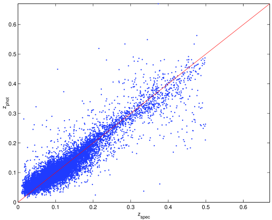
Figure 4: Photometric versus spectroscopic redshifts obtained with a Bayesian MLP with 2 optimization cycles, 50 learning epochs of quasi-Newton algorithm and 5 inner epochs for hyperparameter optimization. Hyperparameters were initialized at $\alpha$=0.001 and $\beta$=50

To be more specific: in the SDSS-EDR spectroscopic sample, over a total of 54,008 objects having $z>0$, only $88\%$, $91\%$ and $93\%$ have redshift $z$ lower than, respectively than $0.3$, $0.5$ and $0.7$. To train the network on objects falling in the above ranges implies , respectively, a minimum fraction of $12\%$, $9\%$ and $7\%$ of objects in the photometric data set having wrong estimates of the photometric redshift. On the other hand, as we have shown, the higher is the cut in redshifts, the lower is the accuracy and a compromise between these two factors needs to be found on objective grounds.

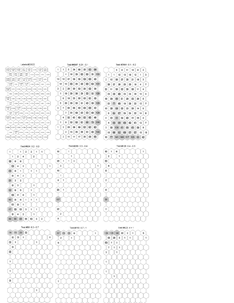
Figure 5: Maps of the neuron activated by the input data set. As before, exagons represent the NN nodes. In the map in the upper left corner, for a given node, the figures n(m) can be read as follows: n is the class (n=1 meaning $z<0.5$ and n=2 meaning $z>0.5$) and m is the number of input vector of the correspondent class which have activated that node. This map was produced using the training and validation data sets. The other maps, produced each in a different redshift bin, indicate how many input vector from the test data set activated a given node.

An accurate estimate of the contamination may be obtained using unsupervised SOM clustering techniques over the training set.

In Figure 5 we show the position of the BMU as a function of the redshift bin. Each exagon represents a neuron and it is clearly visible that low redshift ($z<0.5$) tend to activate neurons in the lower right part of the map, intermediate redshift ones ($0.5<z<0.7$) neurons in the lower left part and, finally, objects with redshift higher than $0.7$ activate only the neurons in the upper left corner. The labeling of the neurons (shown in the upper left map) was done using the training and validation data sets in order to avoid overfitting, while the confidence regions were evaluated on the test set.

Therefore, test set data may be used to map the neurons in the equivalent of confidence regions and to evaluate the degree of contamination to be expected in any given redshift bin. Conversely, when the network is applied to real data, the same confidence regions may be used to evaluate whether a photometric redshift correspondent to a given input vector may be trusted upon or not.

The above derived topology of the network is also crucial since it allows to derive the amount of contamination. In order to understand how this may be achieved, let us take the NN whose topological properties are shown in Figure 5, and consider the case of objects which are attributed a redshifts $z_{phot}$ $<0.5$. This prediction has a high degree of reliability only if the input vector activates a node in the central or right portions of the map. Vector producing a redshift $z_{phot}$ $<0.5$ but activating a node falling in the upper left corner of the map are likely to be misclassified. In Figure 6, we plot the photometric versus spectroscopic redhift for all test set objects having $z_{phot}$ $<0.5$ and activating nodes in the correct region of the map.

As it can be seen, out of 9270 objects with $z_{phot}$ $<0.5$, only 39 (id est, 0.4% of the sample) have discordant spectroscopic redshift. A confusion matrix helps in better quantifying the quality of the results. In Table 3, we give the confusion (or, in this case, ’contamination’) matrix obtained dividing the data in three classes accordingly to their spectroscopic redshifts, namely class I: $0<z<0.3$, class II: $0.3<z<0.5$, class III: $z>0.5$. The elements on the diagonal are the correct classification rates, while the other elements give the fraction of objects belonging to a given class which have been erroneously classified into an other class.

Table 3: confusion matrix for the three classes described in the text.

	objects	Class I	Class II	Class III
Class I	$9017$	$95.4\%$	$2.96\%$	$1.6\%$
Class II	$419$	$6.4\%$	$76.6\%$	$16.9\%$
Class III	$823$	$3.8\%$	$2.1\%$	$94.2\%$

As it can be seen, in the redshift range $(0,0.3)$, 95.4% of the objects are correctly identified and only $4.6\%$ is attributed a wrong redshift estimate. In total, $94.2\%$ are correctly classified. By taking into account only the redshift range $0<z<0.5$, this percentage becomes $97.3\%$. From the confusion matrix, we can therefore derive a completeness of $97.8\%$ and a contamination of about $0.5\%$.

A simple step filter applied to the accepted BMU’s allows therefore to optimise the filter performances. For instance, it allows to choose whether to minimize the number of misclassified objects (thus reducing the completeness) or to minimize the classification error in a given redshift bin more than in another one.

Another possible use of the topological properties of the SOM will be discussed in a forthcoming paper and concerns the use of BMU to choose for each given input vector the optimal NN.

4 Summary and conclusions

The application of NNs to mixed data, id est spectroscopic and photometric surveys, allows to derive photometric redshifts over a wide range of redshifts with an accuracy equal if not better to that of more traditional techniques.

The method makes use of three different neural tools: i) an unsupervised SOM used to cluster the data in the training, validation and test set in order to ensure a complete coverage of the input parameter space; ii) a MLP in Bayesian framework used to estimate the photometric redshifts; iii) a supervised SOM used to derive the completeness and the contamination of the final catalogues. On the SDSS-EDR, the best result (interq. error = 0.020) was obtained by a MLP with 1 hidden layer of 22 neurons, after 5 Bayesian cycles. Once they are trained, NNs are extremely effective in terms of computational costs (the 16 million objects in the SDSS-EDR are processed in less than 50 min on a laptop; Longo et al. 2002, in preparation).

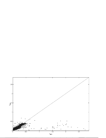
Figure 6: Spectroscopic versus photometric redshifts for objects belonging to Class I and Class II. Outliers are misclassified galaxies.

The method fully exploits the wealth of data provided by the new digital surveys since it allows to take into account not only the fluxes, but also the morphological and photometric parameters.

The proposed method will be particularly effective in mixed surveys, id est, in surveys were a large amount of multiband photometric data is complemented by a small subset of objects having also spectroscopic redshifts. It needs also to be stressed that the foreseen implementation of the Virtual Observatory will provide an ideal framework to NN based data mining tools: the availability of continuously updated data sets from where to extract reliable and extensive training sets will allow a widespread use of supervised NNs for the fast and accurate derivation of secondary parameters such as the photometric redshifts.

References

- Allende Prieto et al. (2000) Allende Prieto C., Rebolo R., Lopez R.J.G., Serra-Ricart M., Beers T.C., Rossi S., Bonifacio P., Molaro P., 2000, AJ, 120, 1516
- Andreon et al. (2001) Andreon S., Gargiulo G., Longo G., Tagliaferri R., Capuano N., 2000, MNRAS, 319, 700
- Bailer and Jones (1998) Bailer-Jones C.A.L., Irwin M., von Hippel T., 1998, MNRAS, 298, 361
- Baum (1962) Baum W.A., 1962, Problems of extragalactic research, IAU Symp. n.15, 390
- (5) Bertin E., Arnout S., 1996, AAS, 117, 393
- Bishop (1995) Bishop C.M., 1995, Neural Networks for Pattern Recognition, Oxford University Press
- Brunner et al. (2000) Brunner R.J., Szalay A.S., Connolly A.J., 2000, ApJ, 541, 527
- Bruzual and Charlot (1993) Bruzual A.G., Charlot S., 1993, ApJ, 405, 538
- Connolly et al. (1995) Connolly A.J., Csabai I., Szalay A.S., Koo D.C., Kron R.G., Munn J.A., 1995, AJ, 110, 2655
- Connolly et al. (1998) Connolly A.J., Szalay A.S., Brunner R.J., 1998, ApJ, 499, L125
- Fernandez-Soto et al. (2001) Fernandez-Soto A., Lanzetta K.A., Chen H.W., Pascarelle S.M., Yakate N., 2001, ApJSS, 135, 41
- Giordano (2001) Giordano G., 2001, ” A neural technique for the analysis of cosmic large scale structure”, Laurea Thesis, November 2001, University of Salerno
- Kohonen (1995) Kohonen T., 1995, Self-Organizing Maps, Springer:Berlin-Heidelberg
- Koo (1999) Koo D.C., 1999, astro-ph/9907273
- Lahav et al. (1996) Lahav O., Naim A., Sodré L. jr., Storrie-Lombardi M.C., 1996, MNRAS, 283, 207
- Le Fèvre et al. (2000) Le Fèvre et al. 2000, in Clowes R.G. et al. eds., ASP. Conf. Ser., New era of Wide Field Astronomy, 232, 449
- Longo et al. (2001) Longo G., Tagliaferri R., Sessa S., Ortiz P, Capaccioli M., Ciaramella A., Donalek C., Raiconi G., Staiano A., Volpicelli A., in Astronomical Data Analysis, J.L. Stark and F. Murtagh eds., SPIE n. 4447, p.61
- MacKay et al. (1994) MacKay et al., Bayesian methods for backpropagation networks models of neural network III, 1994, New York:Springer-Verlag
- (19) Massarotti M., Iovino A., Buzzoni A, 2001a, AA, 368, 74
- (20) Massarotti M., Iovino A., Buzzoni A., Valls-Gabaud D., 2001b, AA, 380, 425
- Nabney and Bishop (1998) Nabney I.T., Bishop C.M., 1998, Netlab: Neural Network Matlab Toolbox, Aston University
- Neal (1994) Neal, R.M., Bayesian Learning for Neural Networks, Ph.D. thesis, 1994, University of Toronto (Canada)
- Pushell et al. (1982) Pushell J.J., owen F.N., Laing R.A., 1982, ApJ, 275, L57
- (24) Storrie-Lombardi M.C., Lahav O., Sodré L. jr, Storrie-Lombardi L.J., 1992, MNRAS, 259, 8
- Stoughton et al. (2001) Stoughton C., Lupton R.H., Bernardi M., Blanton M. R., et al., 2001, AJ, 123, 485
- Tagliaferri et al. (2002) Tagliaferri R., Longo G., Milano L., Ciaramella A., Donalek C., Raiconi G., Volpicelli A., 2002, Neural Networks, in preparation
- Vesanto (1997) Vesanto J., 1997, Ph.D. Thesis, Helsinky University of Technology
- Wang et al. (1998) Wang Y., Bachall N., Turner E.L., 1998, AJ, 116, 2081
- Weaver (2000) Weaver W.B., 2000, ApJ, 541, 298
- York et al. (2000) York D.G., et al. 2000, AJ, 120, 1579