Asymptotic behavior of a stratified perturbation in a three dimensional expanding Universe

The non-linear evolution of a stratified perturbation in a three dimensional expanding Universe is considered. A general Lagrangian scheme (Q model) is introduced and numerical investigations are performed. The asymptotic contraction of the core of the agglomeration is studied. A power-law scaling is detected and an heuristic interpretation of the numerical findings is provided. An asymptotic equation for the multi-stream velocity flow is derived and it is shown to agree quantitatively with the dynamics of the Q model. The relation to the adhesion model is discussed.

1 Introduction

The present Universe is inhomogeneous with structures of many scales, from galaxies to galaxy clusters and superclusters. Around $100000$ years after Big Bang, the Universe was however very nearly homogeneous, with density fluctuations of relative magnitude of about $1:10^{5}$. The presently observed large scale structure have been generated by the process of the gravitational instability, acting on those initially small perturbations.

The goal of this paper is to investigate in direct numerical simulations and theoretical analysis the validity of the adhesion model, a benchmark for the non linear development of the gravitational instability. We will make contact with recent results of Buchert & Domínguez (Buchert1 (1999)) and present a sharpening of their main findings. The conclusion of this study is that the Burgers equation of the adhesion model does not model structure formation quantitatively correctly, but another transport equation of a similar type does.

We will limit ourselves to a flat, critical Universe ($\Omega=1$) where most mass is contained in a dark component. In fact, we assume effectively that all the matter is dark, or behaves as such. There is no vacuum energy, or, equivalently, the cosmological constant is zero. This has been the favored cosmological model in the recent past and, although it is not at the present, it is still of conceptual and qualitative interest. We remark that the approximation of a flat critical Universe will be an accurate one for most of the time since recombination epoch, also in the presently favored models.

We will further make the assumption of stratified perturbations. This is surely not realistic, but, as we will see, it allows for a numerical scheme of incomparable speed and accuracy, describing the full process of structure formation, and is therefore a useful testing ground.

The paper is organized as follows: in Section 2 we present the general background. In Section 3 we recall the derivation of the Quintic model (Aurell & Fanelli Qmodel (2001)), that allows to study the evolution of a stratified perturbation in a Einstein-de Sitter, three dimensional expanding Universe. Section 4 is devoted to the discussion of the numerical implementation. In Section 5 we present the result of our numerical study: scaling laws are displayed and an heuristic explanation is provided. In Section 6 we derive an equation of transport that is consistent with the numerical findings. In the final Section 7 we sum up and discuss our results.

2 General Background

The linear regime of structure formation was studied by Lifshitz Lifshitz (1947) and is described in several classical monographs (Peebles Peebles1980 (1980), Weinberg Weinberg1972 (1972)). For the non linear regime, there is a long tradition of considering various simplified models, from the Zeldovich pancake (Shandarin & Zeldovich Zeldovich (1989)) and the adhesion model ( Gurbatov, Saichev & Shandarin Gurbatov (1989)), to full-scale $N$-body simulations, with the accompanying approximations of numerical nature. We start with a short review of the basic setup and equations.

Collision-less dark matter is described by the kinetic Vlasov-Poisson equations, in an expanding three dimensional Universe. This level of approximations contains the assumption that tensor degrees (gravitational waves) can be neglected, and that the matter motion is quasi-Newtonian. We assume an inertial reference frame, and label the position with ${\bf r}$. Then it is customary to introduce the comoving coordinate ${\bf x}$ by performing the following transformation (Peebles Peebles1980 (1980)):

$${\bf r}=a(t){\bf x}\leavevmode\nobreak\ ,$$ (1)

where the scale factor $a(t)$ is function of proper world time. For the critical Friedman Universe:

$$a=\left(\frac{t}{t_{0}}\right)^{2/3}\leavevmode\nobreak\ ,$$ (2)

and $t_{0}^{-2}=6\pi G\rho(t_{0})$, where $\rho(t_{0})$ is the homogeneous density at time $t_{0}$ (Peebles Peebles1980 (1980), Weinberg Weinberg1972 (1972)) and $G$ is the gravitational constant. The Vlasov-Poisson equations read:

$$\left\{\begin{array}[]{l}\displaystyle{\partial_{t}f+\frac{\bf p}{ma^{2}}\cdot{\bf\nabla_{x}}f-{\bf\nabla_{x}}\psi\cdot{\bf\nabla_{p}}f=0}\\ \\ \displaystyle{\nabla^{2}\psi=4\pi Ga^{2}\left(\rho-\rho_{b}\right)}\leavevmode\nobreak\ ,\end{array}\right.$$ (3)

where ${\bf p}$ is the variable conjugated to ${\bf x}$; $f({\bf x},{\bf p},t)$ is the distribution function in the six dimensional phase space $({\bf x},{\bf p})$; $\psi$ is the gravitational potential and $\rho_{b}$ is the mean mass density distribution. The particle density $\rho({\bf x},t)$ and velocities ${\bf u}({\bf x},t)$ are given, in term of $f({\bf x},{\bf p},t)$, as:

$$\rho({\bf x},t)=\frac{m}{a^{3}}\int f({\bf x},{\bf p},t)d{\bf p}\leavevmode\nobreak\ ,$$ (4)

$$\rho({\bf x},t){\bf u}({\bf x},t)=\frac{1}{a^{4}}\int{\bf p}f({\bf x},{\bf p},t)d{\bf p}.$$ (5)

It is well known that (3) admits special solutions of the form (Vergassola, Dubrulle, Frisch & Noullez Vergassola (1993)):

$$f({\bf x},{\bf p},t)=\frac{a^{3}\rho({\bf x},t)}{m}\delta^{d}({\bf p}-ma{\bf u}({\bf x},t))\leavevmode\nobreak\ ,$$ (6)

where $d$ is the dimension of space and $\delta^{d}(.)$ the $d$-dimensional delta function. We will refer to this class as single-speed solutions, because to each given (${\bf x},t$) corresponds a well defined velocity ${\bf u}$. Assuming (6), after some manipulation, it follows from equations (4) and (5):

$$\left\{\begin{array}[]{l}\displaystyle{\partial_{t}\rho+3\frac{\dot{a}}{a}\rho+\frac{1}{a}{\bf\nabla}\cdot({\rho}{\bf u})=0}\\ \\ \displaystyle{\partial_{t}{\bf u}+\frac{\dot{a}}{a}{\bf u}+\frac{1}{a}({\bf u}\cdot{\bf\nabla}){\bf u}={\bf g}}\\ \\ \displaystyle{{\bf\nabla}\cdot{\bf g}=-4\pi Ga(\rho-\rho_{b})}\leavevmode\nobreak\ ,\end{array}\right.$$ (7)

where we have introduced ${\bf g}=-{\bf\nabla}\psi/a$ such that ${\bf\nabla}\times{\bf g}=0$. It should be stressed that system (7), is valid as long as the distribution function $f({\bf x},{\bf p})$ is in the form (6). Beyond the time of caustic formation, when the fast particles cross the slow ones, the solution become multi-stream. Hence, the pressure-less and dissipation-less hydrodynamical equations (7) are incomplete. We will in this paper extend system (7) beyond caustic formation for stratified flows, i.e. when velocity has one component only, and varies with respect to this direction.

Let us focus now on time before the first particle crossing. Then we can further make the assumption of parallelism: the peculiar velocity is a potential field, which remains parallel to the gravitational peculiar acceleration field (Buchert T., Domínguez A. & Perez-Mércader Buchert2 (1999), Peebles Peebles1980 (1980), Vergassola, Dubrulle, Frisch & Noullez Vergassola (1993)):

$${\bf g}=F(t){\bf u}\leavevmode\nobreak\ ,$$ (8)

where $F(t)$ is a positive, time dependent, proportionality coefficient. Relation (8) is well justified in the linear, as well in the weakly non linear regimes and allows to treat analytically the problem. From the linear theory it follows (Buchert T., Domínguez A. & Perez-Mércader Buchert2 (1999), Peebles Peebles1980 (1980), Vergassola, Dubrulle, Frisch & Noullez Vergassola (1993)):

$$F(t)=4\pi G\rho_{b}b/\dot{b}\leavevmode\nobreak\ ,$$ (9)

where $b$ represents the growing mode of the density field in the linear regime. Hence, defining the new velocity field ${\bf v}={\bf u}/(a\dot{b})$, the system (7) reduces to:

$$\partial_{b}{\bf v}+({\bf v}\cdot{\bf\nabla}){\bf v}=0\leavevmode\nobreak\ ,$$ (10)

which is the multidimensional Burgers equation (Vergassola M., Dubrulle B., Frisch U. & Noullez A. Vergassola (1993)). The inviscid Burgers equation describes the free motion of fluid particles subject to zero forcing and is equivalent to the famous Zeldovich approximation (Shandarin & Zeldovich Zeldovich (1989)). Again, it is worth recalling that the picture is correct as long as the solution stays single-stream. After caustic formation, it has been proposed that the resulting change on the gravitational force can be modeled by an effective diffusive term (adhesion model (Gurbatov S.N., Saichev A.I. & Shandarin S.F. Gurbatov (1989))). This should represent the effect of the gravitational sticking not captured by the Zeldovich approximation. Mathematically, this means introducing a term of the form $\mu\nabla^{2}{\bf v}$, in the right hand side of the equation (10). In order for the diffusion term to have a smoothening effect only in those regions where the particles crossing takes place, the viscosity $\mu$ should be small. The adhesion model reads:

$$\left\{\begin{array}[]{l}\displaystyle{\partial_{b}{\bf v}+({\bf v}\cdot{\bf\nabla}){\bf v}=\mu\nabla^{2}{\bf v}}\\ \\ \displaystyle{{\bf v}=-{\bf\nabla}\tilde{\psi}}\\ \\ \displaystyle{\partial_{b}\rho+{\bf\nabla}\cdot(\rho{\bf v})=0}\leavevmode\nobreak\ .\end{array}\right.$$ (11)

where $\tilde{\psi}=\psi/(\dot{b}F(t))$. The limit when viscosity $\mu$ tends to zero is often taken. We remark, that, as is well known this is not equivalent to setting $\mu$ to zero from the outset, but is instead a regularization of (10), equivalent to the Lax entropy condition.

Although numerical experiments suggest qualitative agreement, no theory is to our knowledge presently available that quantifies the exact relationship between (3) and (11), after caustic formation.

The hypothesis has been put forward that (11) is an asymptotic description of (3), for particular classes of initial conditions (Starobinsky starobinsky (2000)). This statement relies on the assumption that, because of the expansion, the thickness of the individual pancakes grows more slowly than their typical separation. We will refer to this picture as to Starobinsky conjecture. Repeating the statement in the introduction, the aim of this paper is to investigate the asymptotic relation between the Vlasov approach (3) and the adhesion model (11), focusing our attention on the stratified dynamics. To jump also again to the conclusion, we will derive transport equation similar to those of Buchert& Domínguez (Buchert1 (1999)), but not quite the same.

3 Quintic model

We will study stratified perturbation in a critical Universe, in a particle representation. We recall that a non-linear change of time allows us to transform the equations of motion to ordinary differential equations with constant coefficients, and which can therefore be integrated by a fast event-driven scheme. We will refer to this dynamics as to the Quintic model (Aurell & Fanelli Qmodel (2001)), for reason that will become clear.

The Newtonian equations of motion for $N$ particles follow from a Lagrangian

$${\mathcal{L}}=\sum_{i}\frac{1}{2}m_{i}\dot{{r_{i}}}^{2}-m_{i}\phi({r_{i}},t)$$ (12)

where $\nabla_{r}^{2}\phi=4\pi G\rho$. In the point particle picture the density profile is:

$$\rho(x_{i},t)=\sum_{x_{j}}m_{j}a^{-3}\delta(x_{i}-x_{j})\leavevmode\nobreak\ ,$$ (13)

where $x_{i}$ is the comoving coordinate of the $i-th$ particles, in the direction of which the density and velocities varies.

Expressing (12) as function of the proper coordinate, $x_{i}$, and assuming (13), the equation of motion of the $i$-th particle reads:

$$\frac{d^{2}x_{i}}{dt^{2}}+2\frac{\dot{a}}{a}\frac{dx_{i}}{dt}-4\pi G\rho_{b}(t)x_{i}=a^{-3}E_{grav}(x_{i},t)\leavevmode\nobreak\ ,$$ (14)

where

$$E_{grav}(x_{i},t)=-2\pi G\sum_{j}m_{j}\hbox{sign}(x_{i}-x_{j})\leavevmode\nobreak\ .$$ (15)

From the equation of continuity:

$$\rho_{b}(t)=\rho_{0}a(t)^{-3}\leavevmode\nobreak\ ,$$ (16)

and, by performing a suitable non linear transformation of the time variable it is possible to concentrate all the time dependence in the term $2\frac{\dot{a}}{a}\frac{dx_{i}}{dt}$. The choice is:

$$dt=a^{3/2}d\tau\leavevmode\nobreak\ ,$$ (17)

where $\tau$ has dimension of time ( Rouet, Feix & Navet Rouet1990 (1990), Rouet et al. Rouet1991 (1991)). The equation (14) is thus transformed into:

$$\frac{d^{2}x_{i}}{d\tau^{2}}+\frac{\dot{a}\sqrt{a}}{2}\frac{dx_{i}}{d\tau}-4\pi G\rho_{0}x_{i}=E_{grav}(x_{i},\tau)\leavevmode\nobreak\ .$$ (18)

In a flat Einstein de Sitter model the scale factor $a(t)$ grows with time as a power-law (see eq. (2)) and therefore eq. (18) takes the form:

$$\frac{d^{2}x_{i}}{d\tau^{2}}+\frac{1}{3t_{0}}\frac{dx_{i}}{d\tau}-\frac{2}{3t_{0}^{2}}x=E_{grav}(x_{i},\tau)\qquad\hbox{Q model}\leavevmode\nobreak\ .$$ (19)

The possibility of making this coordinate change is indeed the technical reason why we work with a critical Universe. Equation (19) is the model we refer to as to the Quintic (Q) model. We stress that the quintic model is nothing but a particle picture of the full self-gravitating dynamics for the class of stratified perturbations. The continuum ($N\rightarrow\infty$) limit of (19) is just (3), with different time coordinate. The interest of this formulation is that, as for the classical static self-gravitating systems in one dimension, $E_{grav}$ is a Lagrangian invariant, proportional to the net mass difference to the right and to the left of a given particle at a given time. Hence, the evolution of the system is recovered by identifying the time and location of the particles crossings, and connecting analytical solutions between such events (Noullez, Fanelli & Aurell al (2001)).

4 Numerical scheme

The equation of motion of each particle, in the Q model, is specified by equation (19). In between successive crossings ($\tau\in[\tau^{n},\tau^{n+1}]$) the right hand side is a constant and, therefore, (19) admits an explicit solution in the form (Aurell & Fanelli Qmodel (2001)):

$$x_{i}(\tau)=c^{i}_{1}\exp(\frac{2(\tau-\tau^{n})}{3t_{0}})+c^{i}_{2}\exp(-\frac{(\tau-\tau^{n})}{t_{0}})-K_{i}^{n}\leavevmode\nobreak\ ,$$ (20)

where $K_{i}=(3t_{0}^{2}/2)E_{grav}(x_{i},\tau)$, is constant. The coefficients $c^{i}_{1}$ and $c^{i}_{2}$ are determined by $x_{i}^{n}=x_{i}(\tau^{n})$ and $w_{i}^{n}=\dot{x_{i}}(\tau^{n})$, i.e. by the states of the particle at the time of the last crossing, and read:

$$\left\{\begin{array}[]{l}\displaystyle{c^{i}_{1}=\frac{3}{5}\left[x_{i}^{n}+t_{0}w_{i}^{n}-K_{i}\right]}\\ \\ \displaystyle{c^{i}_{2}=\frac{2}{5}\left[x_{i}^{n}-\frac{2}{3}t_{0}w_{i}^{n}-K_{i}\right]}\leavevmode\nobreak\ .\end{array}\right.$$ (21)

The form of equation (20) suggests introducing an auxiliary variable $z=\exp((\tau-\tau^{n})/3t_{0})$. The crossing times between neighboring particles (i.e. $i$,$i+1$) can, hence, be computed by solving numerically a quintic equation in the form:

$$f(z)=A_{i,i+1}^{n}z^{5}-B_{i,i+1}^{n}z^{3}+C_{i,i+1}^{n}=0\leavevmode\nobreak\ ,$$ (22)

where:

$$\left\{\begin{array}[]{l}\displaystyle{A_{i,i+1}^{n}=\frac{3}{5}\left[\Delta x_{i}^{n}+t_{0}\Delta w_{i}^{n}-(K_{i+1}-K_{i})\right]}\\ \\ \\ \displaystyle{B_{i,i+1}^{n}=-(K_{i+1}-K_{i})=const}\\ \\ \displaystyle{C_{i,i+1}^{n}=\frac{2}{5}\left[\Delta x_{i}^{n}-\frac{2}{3}t_{0}\Delta w_{i}^{n}-(K_{i+1}-K_{i})\right]}\leavevmode\nobreak\ ,\end{array}\right.$$ (23)

and $\Delta x_{i}^{n}=x_{i+1}^{n}-x_{i}^{n}$, $\Delta w_{i}^{n}=w_{i+1}^{n}-w_{i}^{n}$. The function $f(z)$ represents the distance between particles $i$ and $i+1$, at transformed time $z$.

The event-driven scheme (Noullez, Fanelli & Aurell al (2001)) can be adopted to follow the dynamics of the system. The positions of the particles are stored in monotonically increasing order. A proper time, $\theta_{i}$, is associated to each particle $i$: it refers back to the time the particle last experienced a collision. Initially all $\theta_{i}$ are set to zero. The algorithm computes first the crossing time of each particle with the neighbor to the right, by solving $N-1$ quintic equations, as in (22) (see above). The results are then stored in an array, which is sorted on a heap. Once the heap has been built, the minimum collision time, $t_{min}$, is at the root, i.e. at the first position in the heap. The particles involved in the first collision are selected by means of a trivial ${\cal O}(1)$ operation. The algorithm lets them evolve up to $t_{min}$, according to the equation (20). At this point, the particles share the same spatial position, and the crossing takes place (the velocities are exchanged). The successive step is to compute the next predicted collision time between $i$ and $i+1$. The new value replaces the old one, and the heap needs to be rearranged. In addition, as an effect of the changes in velocity for particles $i$ and $i+1$ particles, the two collisions with their nearest neighbors (respectively $i-1$ and $i+2$) need to be re-computed. The heap is then re-arranged with at most ${\cal O}(\log(N))$ operations and the whole procedure can be repeated for $N_{coll}$ collisions. Therefore the complexity of the algorithm is in worst-case ${\cal O}(N_{coll}\log(N))$ (Noullez, Fanelli & Aurell al (2001)).

Indeed, in this particular application, the numerical procedure for finding the solution of the quintic equation might converge slowly, affecting the whole computation time, with a non negligible contribution. Therefore, in order to achieve the goal of a fast implementation, special care has to be devoted to the analysis of (22). Recalling the definition of $f(z)$, we look for the smallest real value $\bar{z}>1$, such that $f(\bar{z})=0$. As a first trivial observation, we notice that, by definition, $z$ is larger than one, and the inter-particle distance $f(z=1)$ is non-negative. In addition, $B_{i,i+1}^{n}$ is a positive constant, independent of $i$.

Two scenarios are therefore possible: if the coefficient $A_{i,i+1}^{n}$ is positive, no crossing is allowed. As it is sketched in Fig. 1, the only real root of eq. (22) lies in the interval $[0,1]$, and therefore has to be rejected.

Figure 1: The function $f(z)$ represented versus $z$, for $A_{i,i+1}^{n}$ positive. The solid line refers to the case when $C_{i,i+1}^{n}$ is positive while the dashed line to $C_{i,i+1}^{n}$ negative. Note that no intersection with the horizontal axis is allowed for $z>1$ (since $f(1)>0$, by definition).

This means that these two particles will never collide if left to themselves: the expansion is too strong to be overcome by their mutual gravitational attraction.

On the other hand, if the coefficient $A_{i,i+1}^{n}$ is negative, more care is required. The problem is to bound the root in a reasonable interval in order to assure a fast convergence of a numeric procedure. First, we observe that there is a local maximum for $z>0$. The coordinate $z_{max}$ is easily computed and $f(z_{max})$ is evaluated; $f(z_{max})$ is positive, since it is by definition larger of $f(1)>0$. Since the function $f(z)$ goes to $-\infty$ as $z\rightarrow\infty$, there should be an intersection ($\bar{z}>1$ s.t. $f(\bar{z})=0$) with the horizontal axis, see Fig 3.

Figure 2: The function $f(z)$ represented versus $z$, for $A_{i,i+1}^{n}$ negative (thick solid line). The thin solid line represents the quadratic approximation around $z=z_{max}$. Here $f(z_{1})$ is negative and, therefore, the root $\bar{z}$ is bounded between $[z_{max},z_{1}]$.

The following procedure is adopted. First we introduce $h(z)$ (thin solid line in Figs. 2, 3), that is the quadratic approximation of $f(z)$ around $z_{max}$, defined by:

$$h(z)=f(z_{max})+\frac{1}{2}f^{{}^{\prime\prime}}(z_{max})(z-z_{max})^{2}\leavevmode\nobreak\ .$$ (24)

Then we compute the intersection $z_{1}$ of $h(z)$ with the horizontal axis:

$$z_{1}=z_{max}+\left(\frac{f(z_{max}}{3B_{i,i+1}^{n}}\right)\sqrt{\frac{-5A_{i,i+1}^{n}}{3B_{i,i+1}^{n}}}\leavevmode\nobreak\ .$$ (25)

Two different cases have to be considered (respectively, Figs. 2,3).

Figure 3: The function $f(z)$ represented versus $z$, for $A_{i,i+1}^{n}$ negative (thick solid line). The thin line is the quadratic approximation around $z=z_{max}$. Here $f(z_{1})$ is positive and therefore, the root $\bar{z}$ is bounded between $[z_{1},z_{2}]$. Here $z_{2}$ is the intersection with the $z$ axis of the tangent to $f(z)$ in $z_{1}$ (dotted line).

If $f(z_{1})$ is positive, we take the tangent to $f(z)$ in $z_{1}$, and compute its intersection, $z_{2}$, with the $z$ axis (Fig. 3):

$$z_{2}=z_{1}-\frac{f(z_{1})}{5A_{i,i+1}^{n}z_{1}^{4}+3B_{i,i+1}^{n}z_{1}^{2}}\leavevmode\nobreak\ .$$ (26)

By construction $z_{2}>\bar{z}$ and, therefore, $\bar{z}\in[z_{1},z_{2}]$. If, on the contrary, $f(z_{1})$ is negative, then $\bar{z}\in[z_{max},z_{1}]$, see Fig. 2.

In both cases we have confined the root in a narrow interval: there, $f(z)$ is a monotonic decreasing function. Therefore, we can apply a combination of bisection and Newton-Rapson method (Press num (1992)). This hybrid algorithm assures a stable and fast convergence to the solution. In the present implementation we assumed a tolerance error of $10^{-13}$.

5 Asymptotic scaling laws: numerical results and heuristic interpretation

We simulate the dynamics of the Q model, by using the numerical scheme discussed above. We consider a system of $N$ particles of mass $m=1/N$, confined in a box of size $L$. Reflecting boundary conditions are assumed, which is equivalent to consider periodic perturbation of size $2L$, with reflexion symmetry (Aurell & Fanelli Qmodel (2001)). We choose units such that $4\pi G$ is equal to one. Time is measured by the a-dimensional quantity $(t/t_{0})$. The unit of length is the spatial interval in which the particles are initially distributed (i.e. $L=1$), and thus the initial density $\rho_{0}$ is set to one.

In particular, we are interested in the late time evolution of the system to better understand the validity of the Starobinsky conjecture, the aim of this analysis being to provide a quantitative test of the reliability of the adhesion model, as an effective description of the mechanism of large scale structure formation in the Universe.

With this in mind, we consider the evolution of an individual cluster and investigate the process of gravitational collapse. We measure the progressive contraction of the inner region of the agglomeration, compared to the overall expansion. This effect can be computed by the ratio between the width of region, $\Delta x$, that contains half of the whole mass of the system, centered around the position of maximum density, and the size of the perturbation $L$ . This quantity is then plotted, as function of the rescaled cosmological time $t/t_{0}$.

Simulations are performed for two different classes of initial conditions. In both cases, we make the non restrictive choice of considering a perturbation centered around our center of reference.

First, the initial velocity is assumed to be a smooth function of position. As clearly expected, the system develops spiral in the phase space like the one displayed in Fig. 4.

Figure 4: Velocity field versus positions, starting from a single speed initial condition (sinus wave). Here $N=4096$ and $t/t_{0}=6.1249064\times 10^{4}$. Reflecting boundaries are assumed. Positions and velocities are in arbitrary units.

In Fig. 5 we plot $\Delta x/L$, versus $t/t_{0}$. The experiments are performed for different values of $N$. A clear power-law behavior:

$$\frac{\Delta x}{L}=\left(\frac{t}{t_{0}}\right)^{\alpha}$$ (27)

is always displayed, regardless of the number of particles simulated. This implies that the result is not affected by the discreteness of the representation, and can be assumed to hold in the continuum limit. The scaling is present over several decades and the best numerical fit gives the value $\alpha=-0.22$.

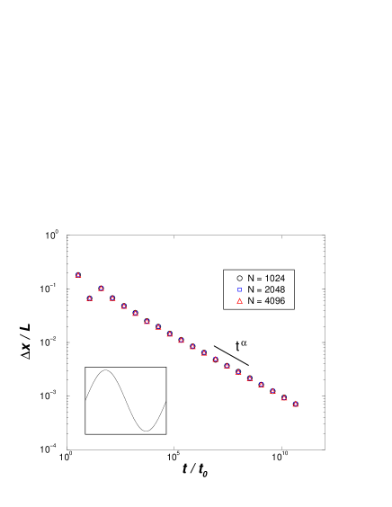
Figure 5: $\Delta x/L$ is plotted versus $t/t_{0}$. Different symbols refer to different values of $N$ (see the legend). A clear power-law behavior is displayed. The best numerical fit gives exponent $\alpha=-0.22$. The small inset represent the initial condition in the phase space $(x,w)$.

Then, a source of noise is introduced in the initial condition: as shown in the small inset of Fig. 6 a white noise signal is generated and superposed to a sinus wave of amplitude $w_{0}$. The thickness of the dense region is studied, following the line of the preceding discussion. Results are reported in the main plot of Fig. 6, for a single realization. They show complete agreement with (5) .

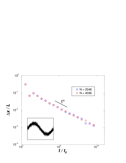
Figure 6: $\Delta x/L$ is plotted versus $t/t_{0}$. Here $w_{0}$ represents the amplitude of the initial smooth sinus to which the white noise, $s_{wn}$, is superposed (i.e., $w=w_{0}sin(x)+s_{wn}$, see small inset). Different symbols refer to different values of $N$ (see the legend). The scaling is consistent with the one derived from Fig. 5 (here represented by the thick solid line).

It is worth stressing that these results are not sensitive to the choice of measuring the interval that contains $N/2$ particles. Any other finite fraction leads to the same conclusions.

In order to provide a full picture, we performed similar analysis for the velocities distribution. Consider $\Delta w$, such that $N/2$ particles have velocities in the interval $[\Delta w/2,-\Delta w/2]$. The ratio $\Delta w/w_{0}$ is plotted vs. $t/t_{0}$, where $w_{0}$ represents the amplitude of the initial smooth wave (see captions of Figs. 7 and 8). Again, and for both the initial conditions considered here, a power-law behavior:

$$\frac{\Delta w}{w_{0}}=\left(\frac{t}{t_{0}}\right)^{\beta}$$ (28)

is clearly displayed (Figs. 7, 8). Here the best numerical fit gives $\beta=-0.11$.

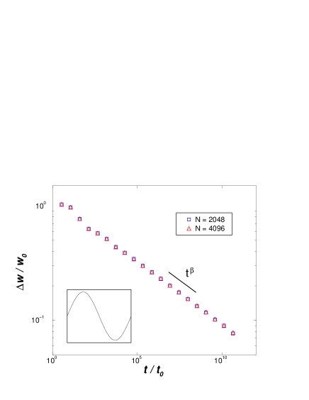
Figure 7: $\Delta w/w_{0}$ is plotted versus $t/t_{0}$. Here $w_{0}$ represents the amplitude of the initial velocity perturbation (i.e., $w=w_{0}\sin(x)$, see small inset). Different symbols refer to different values of $N$ (see the legend). A clear power-law behavior is displayed. The best numerical fit gives exponent $\beta=-0.11$

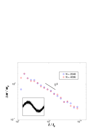
Figure 8: $\Delta w/w_{0}$ is plotted versus $t/t_{0}$. Here $w_{0}$ represents the amplitude of the initial smooth sinus to which the white noise, $s_{wn}$, is superposed (i.e., $w=w_{0}\sin(x)+s_{wn}$, see small inset). Different symbols refer to different values of $N$ (see the legend). The scaling is consistent with the one derived from Fig. 7 (here represented by the thick solid line).

Assuming the occurrence of power-law behaviors, there is a simple, heuristic, explanation for deriving the correct value of the exponents, in agreement with the numerical findings. As previously stated, the Quintic model is equivalent to the Vlasov-Poisson set of equations in the continuous limit (Aurell & Fanelli Qmodel (2001)). Such a system is conservative and therefore the volumes in the phase space are conserved (Liouville theorem). Hence:

$$\Delta x\Delta p=const\leavevmode\nobreak\ ,$$ (29)

where $\Delta x$ and $\Delta p$ represent, respectively, any space and momentum intervals in the comoving reference frame.

Recalling that $w=dx/d\tau$ and that $a(t)=(t/t_{0})^{2/3}$, eq. (29) is transformed into:

$$\Delta x\Delta w=\left(\frac{t}{t_{0}}\right)^{-1/3}\leavevmode\nobreak\ .$$ (30)

Assuming that $\Delta x$ and $\Delta w$ scales in time as power-laws, respectively with exponents $\alpha$ and $\beta$ it follows that:

$$\alpha+\beta=-\frac{1}{3}\leavevmode\nobreak\ .$$ (31)

A second relation is needed to close the system. Let us consider the Hamiltonian $H=K+V$ which describes the Quintic model, except the friction term. $K$ is a normal kinetic term, quadratic in the velocities, and $V$ is made of two terms: the interaction and the background potential. The following relation holds:

$$\frac{dH}{dt}=-\frac{2}{3t_{0}}K\leavevmode\nobreak\ .$$ (32)

Assume that the global virialization has occurred. Then $<K>\sim<V>$, where $<K>$ and $<V>$ represent the time average of the kinetic and potential energies. $K$ is quadratic in velocities while $V$ has one term quadratic (the background), and one linear (the interaction). If we have a mass concentration at the origin, the quadratic can be ignored compared to the linear.

Hence, neglecting the time averages, we have $velocities^{2}\sim distances$. If $\Delta x\sim(t/t_{0})^{\alpha}$, therefore $\Delta w\sim(t/t_{0})^{\alpha/2}$, which implies:

$$\beta=\frac{\alpha}{2}\leavevmode\nobreak\ ,$$ (33)

and therefore $\alpha=-2/9$ and $\beta=-1/9$, in agreement with the numerics. From eq. (32), the dissipative time is:

$$T_{diss}=H/(dH/dt)\sim constant\leavevmode\nobreak\ .$$ (34)

The virialization time of the mass agglomeration, $T_{vir}$ is about the time it takes one particle to traverse the mass, that is

$$T_{vir}=(distance)/(velocity)\sim\left(\frac{t}{t_{0}}\right)^{\beta}\leavevmode\nobreak\ .$$ (35)

Hence, the virialization time becomes quickly smaller than the dissipative time, and the argument is self-consistent.

6 Transport equation

As already observed, relation (6) holds as long as the solution stays single stream. Hence the hydrodynamical picture (7) is applicable just before the time of caustic formation, when the first particles crossing takes place. In order to extend the analysis beyond that time we have to consider the more general solution to (3):

$$f({\bf x},{\bf p},t)=\frac{a^{3}\rho({\bf x},t)}{m}f_{0}({\bf x},{\bf p},t)\leavevmode\nobreak\ .$$ (36)

where $f_{0}({\bf x},{\bf p},t)$ is the velocity profile.

Assuming (36) and performing the same analysis as described in Section 1, the following system is derived from Vlasov-Poisson equations (3):

$$\left\{\begin{array}[]{l}\displaystyle{\partial_{t}\rho+3\frac{\dot{a}}{a}\rho+\frac{1}{a}{\bf\nabla}\cdot\left({\rho}{\bf\overline{u}}\right)=0}\\ \\ \displaystyle{\partial_{t}{\bf\overline{u}}+\frac{\dot{a}}{a}{\bf\overline{u}}+\frac{1}{a}\left({\bf\overline{u}}\cdot{\bf\nabla}\right){\bf\overline{u}}={\bf g}-\frac{1}{a\rho}{\bf\nabla}\left[\rho(\overline{{\bf u}^{2}}-{\bf\overline{u}}^{2})\right]}\\ \\ \displaystyle{{\bf\nabla}\cdot{\bf g}=-4\pi Ga(\rho-\rho_{b})}\leavevmode\nobreak\ ,\end{array}\right.$$ (37)

where $\overline{[\leavevmode\nobreak\ \cdot\leavevmode\nobreak\ ]}$ represents the mean, after averaging over velocity space. Comparing with (7), we see that in the second equation of (37) an extra-term appears, that takes into account the effect of the dispersion in velocities, in the region where the multi-values solution is developed. When the flow is single-stream, the variance is zero and the system (37) is identical to (7) (${\bf\overline{u}}\equiv{\bf u}$). This derivation was already discussed in (Buchert & Domínguez Buchert1 (1999)) and represents the starting point of our analysis. We will limit ourselves to the case of stratified perturbations, and derive an equation for the transport of the velocity flow, that agrees with the numerical analysis performed at the level of the Q model (i.e. discrete Vlasov). In this respect, we are mainly concerned by the progressive collapse of the inner bulk (see Figs 5,6), a key feature that needs to be considered explicitly in our analysis. The question that naturally arises is whether or not the transport is well represented by Burgers’ equation. Here on, we will indicate the mean velocity simply with ${\bf u}$.

Let us consider the dynamics of the Q model. It can be shown numerically that, for all classes of initial conditions here considered, far beyond the time of first crossing, the multi-stream velocity profile $f_{0}(w)$ is well approximated by a Gaussian:

$$f_{0}(w)\propto\exp(-\frac{\left(w-\overline{w}\right)^{2}}{T(x)})\leavevmode\nobreak\ ,$$ (38)

where the temperature , $T(x)$, is smaller in the bulk (more narrow Gaussian) than in the surrounding regions (larger profile). Equation (38) is also, of course, the natural choice in a system close to equilibrium, where $\rho$,$w$ and $T$ vary considerably over a cluster, but little over distances of the order of inter-particle spacing.

Our ansatz for $T(x)$ is the following:

$$T(x)=K\frac{(t/t_{0})^{\xi}}{\rho^{\gamma}}\leavevmode\nobreak\ ,$$ (39)

where $K$ is a constant and $\gamma$ is a real number belonging to the interval $[0,1]$. This choice reproduces qualitatively the shrinking of the velocity profile, observed in comoving coordinates in correspondence of the denser inner regions. On a more quantitative level, numerical checks have been performed to support the validity of (39), showing in all cases, a satisfactory agreement. In particular, from (38) it follows that the variance, $var^{Q}(x)$, is given by:

$$var^{Q}(x)=\overline{w^{2}}-\overline{w}^{2}=\frac{K}{2}\frac{(t/t_{0})^{\xi}}{\rho^{\gamma}}\leavevmode\nobreak\ ,$$ (40)

where the label $Q$ indicates that we work in Quintic variables. In the main plot of figure (9) $var^{Q}(x)$ is plotted versus $x$. The filled circles refers to the results of the numerical experiments, while the solid line is a two parameters fitting, based on (39). (i.e. $var^{Q}(x)=A_{1}/\rho^{A_{2}}$, where now $\rho$ is the histogram of positions and $A_{1},A_{2}$ free parameters). In Fig. 9, $A_{2}=0.3$: the same value, within the errors ($\sim 0.1$), is found for different initial realizations and/or different times.

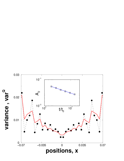
Figure 9: Main plot: $var^{Q}(x)$ is plotted versus $x$. Here $N=8192$ and $t/t_{0}=6.1249064\times 10^{4}$. The filled circles refers to the numerical experiment. The dashed line is a guide to the eye. The solid line is obtained by making use of the fitting function $A_{1}/\rho^{A_{2}}$, with $A_{1},\leavevmode\nobreak\ A_{2}$, free parameters (refer to text for a more detailed description). Here $A_{2}=0.3$. The small inset represents $A_{1}$ vs $t/t_{0}$ (squares), obtained keeping $A_{2}=0.3$ fixed. The solid line is a power-law fit that gives exponent $\xi=-0.22\sim-2/9$.

Larger deviations from (40) are observed outside the core, where the density reduces drastically and the multi-stream flow approaches the single stream limit. The squares in the small inset represent, in double logarithmic scale, the amplitude $A_{1}$ resulting from the fit (keeping now $A_{2}=0.3$) , for different times. The power-law scaling is clear and the exponent is $\xi=-0.22\sim-2/9$. We will come back on this important point in the end of the Section.

Now, let us consider the system (37). Following the discussion in Section 1, we perform the change $v\rightarrow u/a\dot{b}$ and define the new time variable $b$. Then the second equation of (37) reads:

$$\partial_{b}v+\left(v\partial_{x}\right)v=\Gamma^{B}(x,v)\leavevmode\nobreak\ ,$$ (41)

where $\Gamma^{B}(x,v)$ given by:

$$\begin{array}[]{c}\Gamma^{B}(x,v)=-\frac{1}{a^{2}\dot{b}\rho}\partial_{x}\left[\rho\leavevmode\nobreak\ var^{B}(x)\right]=\\ \\ -\frac{9}{4a^{4}\dot{b}\rho}\partial_{x}\left[\rho\leavevmode\nobreak\ var^{Q}(x)\right]\leavevmode\nobreak\ .\end{array}$$ (42)

Here $B$ indicates that the quantity is expressed in Burgers-like variables, i.e. $(x,v,b)$. In (42) the transformation $w\rightarrow\frac{2}{3}a(t)v$ has been considered explicitly. From equation (40) we obtain:

$$\Gamma^{B}(x,v)=-\frac{9K}{8}\frac{(t/t_{0})^{\xi}}{a^{4}\dot{b}^{2}\rho}\partial_{x}\left[\frac{1}{\rho^{\gamma-1}}\right]\leavevmode\nobreak\ .$$ (43)

Inserting the assumption of parallelism (9), the Poisson equation (the third of (37)) reads:

$$\partial_{x}\rho=\frac{F(t)}{4\pi Ga}\partial_{xx}u=-\rho_{b}b\partial_{xx}v\leavevmode\nobreak\ .$$ (44)

Hence equation (43) is transformed into:

$$\Gamma^{B}(x,v)=-\frac{9K}{8}\frac{b(t/t_{0})^{\xi}}{a^{4}\dot{b}^{2}}\frac{\rho_{b}}{\rho^{\gamma+1}}\partial_{xx}v\leavevmode\nobreak\ .$$ (45)

In addition the following relation holds:

$$\frac{1}{\rho^{\gamma+1}}=\frac{1}{\rho_{b}^{\gamma+1}}\left[\frac{1}{1-b\partial_{x}v}\right]^{\gamma+1}\leavevmode\nobreak\ ,$$ (46)

and, thus:

$$\Gamma^{B}(x,v)=-\frac{9K}{8}(\gamma-1)\frac{(t/t_{0})^{\xi}}{a^{4-3\gamma}\dot{b}^{2}}\frac{1}{\rho_{0}}\partial_{x}\left[\frac{1}{1-b\partial_{x}v}\right]^{\gamma}\leavevmode\nobreak\ ,$$ (47)

where we made use of equation (16). Collecting together, equation (41) reads:

$$\partial_{b}v+\left(v\partial_{x}\right)v=\mu(t)\partial_{x}\left[\frac{1}{1-b\partial_{x}v}\right]^{\gamma}\leavevmode\nobreak\ ,$$ (48)

where $\mu(t)$ is a time dependent coefficient defined by:

$$\mu(t)=-\frac{9K}{8}(\gamma-1)\frac{(t/t_{0})^{\xi}}{a^{4-3\gamma}\dot{b}^{2}}\frac{1}{\rho_{0}}=a_{1}\left(\frac{t}{t_{0}}\right)^{\alpha(\xi,\gamma)}\leavevmode\nobreak\ .$$ (49)

Equation (48) is defined in the inner region where the ansatz (39) applies and where the gradient of $v$ is negative. We stress that, even though obtained in a different manner, (48) belongs to the same family of equations derived by ( Buchert, Domínguez & Perez-Mércader Buchert2 (1999)), except for a slight modification of $\mu(t)$ and a different interpretation of $\gamma$. More important, using the constraints imposed by the results in section 4, we will provide a precise indication of the values of $\gamma$ and $\xi$. We therefore proceed to select one candidate from the whole family (48).

Consider equation (48) and apply the following rescaling for position, velocity and time:

$$x=\left(\frac{t}{t_{0}}\right)^{\lambda_{1}}\tilde{x}\leavevmode\nobreak\ ,\leavevmode\nobreak\ \leavevmode\nobreak\ \leavevmode\nobreak\ \leavevmode\nobreak\ \leavevmode\nobreak\ v=\left(\frac{t}{t_{0}}\right)^{\lambda_{2}}\tilde{v}\leavevmode\nobreak\ ,\leavevmode\nobreak\ \leavevmode\nobreak\ \leavevmode\nobreak\ \leavevmode\nobreak\ \leavevmode\nobreak\ db=\left(\frac{t}{t_{0}}\right)^{\delta}d\tilde{b}\leavevmode\nobreak\ .$$ (50)

Equation (48) is transformed into:

$$\begin{array}[]{c}\partial_{\tilde{b}}\tilde{v}+\frac{3}{2}\lambda_{2}\left(\frac{t}{t_{0}}\right)^{\delta-2/3}\tilde{v}+\left(\frac{t}{t_{0}}\right)^{\lambda_{2}-\lambda_{1}-\delta}\tilde{v}\partial_{\tilde{x}}\tilde{v}=\\ \\ a_{1}\left(\frac{t}{t_{0}}\right)^{\alpha(\xi,\gamma)-\lambda_{1}-\delta-\lambda_{2}}\partial_{\tilde{x}}\left[1-\left(\frac{t}{t_{0}}\right)^{2/3-\lambda_{1}+\lambda_{2}}\partial_{\tilde{x}}\tilde{v}\right]^{-\gamma}\leavevmode\nobreak\ .\end{array}$$ (51)

By setting $\lambda_{1}=\alpha/2+2/3$, $\lambda_{2}=\alpha/2$ and $\delta=-2/3$, equation (51) simplifies:

$$\partial_{\tilde{b}}\tilde{v}+\frac{3}{2}\lambda_{2}\tilde{v}+\tilde{v}\partial_{\tilde{x}}\tilde{v}=a_{1}\partial_{\tilde{x}}\left[\frac{1}{1-\partial_{\tilde{x}}\tilde{v}}\right]^{\gamma}\leavevmode\nobreak\ .$$ (52)

All the coefficients are now time independent. Hence, equation (52) develops shocks of constant width, $\Delta\tilde{x}_{shock}$. Transforming back to the old variables, this implies:

$$\Delta x_{shock}=\left(\frac{t}{t_{0}}\right)^{\alpha/2+2/3}\cdot\Delta\tilde{x}_{shock}\propto\left(\frac{t}{t_{0}}\right)^{\alpha/2+2/3}\leavevmode\nobreak\ .$$ (53)

In order to provide a full consistent picture, we require the shock interval to shrink in time with the same rate that have been shown to hold for the discrete Vlasov equation (Q model). Therefore we have to impose:

$$-\frac{2}{9}=\frac{\alpha}{2}+\frac{2}{3}\leavevmode\nobreak\ ,$$ (54)

that implies the following relation between $\gamma$ and $\xi$:

$$\gamma=-\frac{1}{2}\xi+\frac{1}{9}\leavevmode\nobreak\ .$$ (55)

Let us now consider the results reported in Fig. 9. Assuming $\xi=-2/9$ (see analysis above and small inset in Fig. 9), from equation (55) one gets $\gamma=2/9$ that is in agreement with the result of the numerical fitting. Therefore we are led to conclude that asymptotically, the evolution a of multi-stream flow originated by the one-dimensional Vlasov-Poisson dynamics, is mimicked by a transport equation in the form:

$$\partial_{b}v+v\partial_{x}v=\mu(t)\partial_{x}\left[\frac{1}{1-b\partial_{x}v}\right]^{2/9}\leavevmode\nobreak\ ,$$ (56)

where $\mu(t)\propto(t/t_{0})^{-16/9}$ and $b=(t/t_{0})^{2/3}$. As we will show in the next paragraph, the adhesion model can be recovered from our ansatz (39) with a special choice of $\gamma$. Nevertheless both the value of $\gamma$ and the consequent rate of compression of $\Delta x_{shock}$ are not consistent with the numerical study of the Q model reported in Section 4. We are therefore led to conclude that the Burgers’ equation, in the limit of vanishing viscosity, is only valid as a qualitative test model and that, on the other hand, the more quantitative phenomenology is, instead, captured by the transport equation (56).

6.1 The adhesion model: limit of validity

Let us consider the family of equations (48) derived from the ansatz (39). Assume $\gamma=-1$: this is the only possible choice to recover a Burgers like equation, according to our approach. In fact equation (48) then reads:

$$\partial_{b}v+\left(v\partial_{x}\right)v=b\mu(t)\partial_{xx}v\leavevmode\nobreak\ ,$$ (57)

where $\mu(t)=a_{1}\left(\frac{t}{t_{0}}\right)^{\xi-4}$.

There are two major problems with that result. First the choice of $\gamma$ is not consistent with the simulations for the Quintic model. In fact, if $\gamma<0$, the width of the Gaussian profile (38) decreases moving to region of lower density. That is the opposite of what we observed. Moreover, since $\xi=-0.22\sim-2/9$ (see figure 9), $\mu(t)$ decays too fast to agree with the contraction of $\Delta x$ detected with the discrete Vlasov approach .

Hence, equation (57), directly derived from (3), with the assumption (39) fails in reproducing the essence of peculiar aspects of the dynamics, that have been shown to hold in the Vlasov like picture. Nevertheless, as already stressed by (Buchert, Domínguez & Perez-Mércader Buchert2 (1999)), one should note that the viscous like term vanish as $t\rightarrow\infty$ and therefore, at least from a qualitative point of view, the Starobinsky conjecture is justified (formally replacing $\nu\rightarrow 0$ in (11) with $t\rightarrow\infty$).

7 Conclusions

In this paper we discussed the problem of structure formation in a three-dimensional expanding Universe, focusing on stratified perturbations, in a pressure-less medium. This is done by using extensively the Q model, a Lagrangian representation that was derived in a recent paper (Aurell & Fanelli Qmodel (2001)). The Q model is valid in the limit where Newtonian mechanics applies and it is shown to be equivalent to the Vlasov-Poisson equations for $N\rightarrow\infty$.

In particular we investigated the asymptotic behavior of an initial smooth perturbation, by measuring the progressive contraction of the inner region, compared to the overall expansion. Clear power-law scalings are detected and a heuristic explanation is provided. Then we derived an asymptotic transport equation for the velocity, consistent with these observations. By means of a combined numerical and analytical procedure, we obtained equation (56). Moreover, we showed that the Burgers equation with vanishing viscosity, can be directly derived from the kinetic theory, by assuming the ansatz (39). Nevertheless, equation (57) fails in reproducing the correct asymptotic scaling observed and, therefore, we are led to conclude that the adhesion approach is valid only as an approximate model of structure formation. In fact, even though Burgers’ equation holds outside the shocks, the adhesion picture is shown to agree, only at a qualitative level, with the correct Vlasov description, in the massive cores. On the contrary, inside the shocks, the more quantitative phenomenology is captured by the transport equation (56).

- (1) Aurell, E. & Fanelli, D. 2001, submitted to Europ. Phys. Jour. B, cond-mat/0106444
- (2) Buchert T. & Domínguez A. 1999, A&A , 335, 395
- (3) Buchert T., Domínguez A. & Perez-Mércader 1999, A&A , 349, 343
- (4) Fanelli D., Aurell E. & Noullez A. 2001, Proceeding of IAU Symposium 208
- (5) Gurbatov S.N., Saichev A.I. & Shandarin S.F. 1989, MNRAS, 236, 385
- (6) Lifshitz E. 1947, J. Phys. USSR, 10, 116
- (7) Noullez A., Fanelli D. & Aurell E., 2001 submitted to Journ. Comp. Phys., cond-mat/0101336
- (8) Peebles P.J. 1980, The Large-scale Structure of the Universe, (Princeton University Press, Princeton, NJ)
- (9) Press, H.W., Numerical Recipes in Fortran 1992, (Cambridge University Press, Cambridge)
- (10) Rouet J.L., Feix M.R. & Navet M. 1990, Vistas in Astronomy, 33, 357
- (11) Rouet J.L. et al 1991, in Lecture Notes in Physics: Applying Fractals in Astronomy, 161
- (12) Shandarin S.F. & Zeldovich Ya.B. 1989, Rev. Mod. Phys., 61, 185
- (13) Starobinsky A. 2000, Private Communication to U. Frisch
- (14) Vergassola M., Dubrulle B., Frisch U. & Noullez A. 1993, A&A, 289, 325.
- (15) Weinberg S. 1972, Gravitation and Cosmology (Wiley)