Local characteristic algorithms for relativistic hydrodynamics

Abstract

Numerical schemes for the general relativistic hydrodynamic equations are discussed. The use of conservative algorithms based upon the characteristic structure of those equations, developed during the last decade building on ideas first applied in Newtonian hydrodynamics, provides a robust methodology to obtain stable and accurate solutions even in the presence of discontinuities. The knowledge of the wave structure of the above system is essential in the construction of the so-called linearized Riemann solvers, a class of numerical schemes specifically designed to solve nonlinear hyperbolic systems of conservation laws. In the last part of the review some astrophysical applications of such schemes, using the coupled system of the (characteristic) Einstein and hydrodynamic equations, are also briefly presented.

1 Introduction

The numerical investigation of the Einstein equations is nowadays an important and fruitful line of research in general relativity. There exist a number of mathematical formulations of the gravitational field equations which are on the basis of all numerical approaches. The level accomplished in the understanding of these equations, both mathematically and numerically, is high enough to allow, in principle, for sound numerical approaches. Nevertheless, apart from some remarkable results, such as the discovery of critical phenomena by Choptuik choptuik93 or, more recently, the achievement of long-term stable three-dimensional null cone evolutions of single black hole spacetimes gomez98 , the numerical investigations have only partially succeeded, quite understandably due to the complexity of the theory, in providing global numerical solutions of generic spacetimes, especially in the presence of curvature singularities. Traditionally, the formulation which has received the greatest attention by numerical relativists has been the so-called 3+1 (ADM) formulation lichnerowitz ; choquet ; arnowitt (see also the recent review by Friedrich and Rendall friedrich and references therein). This formulation of the Einstein equations as a Cauchy (initial value) problem, along with its multiple variants - hyperbolic (see, e.g. reula and references therein) and conformal reformulations shibata ; baumgarte - is still today the workhorse of numerical relativity (for an up-to-date summary of the status of numerical approaches in 3+1 see, e.g. seidel and references therein.)

On the other hand, despite being known for about forty years now bondi ; sachs ; penrose , the characteristic formulation of the Einstein equations has however been used by much less research groups in numerical relativity (see the recent review by Winicour winicour ). And research programs to integrate numerically the conformal equations friedrich2 have started only more recently huebner1 ; frauendiner ; huebner2 . Compared to the 3+1 formulation, the latter two formulations are best suited to study the conformal structure of the spacetime - the main topic of the workshop -, and the propagation of radiation fields within the spacetime. State-of-the-art numerical methodology applied to such two formalisms is comprehensively reviewed in the corresponding articles by Bartnik and Lehner (characteristic equations) and Frauendiener, Husa and Schmidt (conformal equations) in this volume. Apart from some test computations involving matter sources presented in Lehner’s article, those papers are mainly concerned with the integration of the vacuum field equations.

The present contribution to this volume aims, on the other hand, at describing the current status of the numerical integration of the hydrodynamic equations on curved spacetimes, complementing, to some extent, the contributions by the above authors. Even though the description will be rather basic and general, I will also present some applications and some recent results obtained with the coupled integration of the Einstein and hydrodynamic equations within the framework of the characteristic formulation of the gravitational field equations. It is worth pointing out that, while initially the characteristic evolution of matter was limited to idealized systems such as massless scalar fields, nowadays it is mature enough to account for fully hydrodynamical evolutions with perfect fluids dubal ; bishop ; pf2000 ; pf2001 ; felix ; florian .

Admittedly, the motivation to develop the capabilities to perform coupled evolutions of the matter fields and the geometry needs really not much of an emphasis. In astrophysics general relativity plays a major role in the description of compact objects in such diverse scenarios as core collapse supernovae, black hole formation, accretion, gamma-ray bursts and coalescing compact binaries. With the exception of the coalescence and merging of two black holes - the number one problem of nowadays’ numerical relativity - all realistic astrophysical systems and sources of (detectable) gravitational radiation involve matter.

The only means to study the time-dependent evolution of fluid flow coupled to geometry is through numerical simulations. Some scenarios can be properly described in the so-called ‘test fluid’ approximation, where the self-gravity of the fluid is neglected. Nowadays there is a large body of numerical investigations in the literature dealing with such hydrodynamical integrations in static background spacetimes (see, e.g., references in fontlr ). Most of these are based on the pioneering formulation of the hydrodynamic equations by Wilson wilson and use numerical schemes based on finite differences with some amount of artificial viscosity. The use of conservative formulations of the equations, and their characteristic information, in the design of numerical schemes started in more recent years mim .

On the other hand, time-dependent simulations of self-gravitating flows in general relativity, evolving the spacetime dynamically with the Einstein equations coupled to a hydrodynamic source, are more scarce. Although there is much recent interest in this direction, only the spherically symmetric case has been extensively studied thus far (since the pioneering work of May and White in 1966 maywhite ). In axisymmetry, fewer attempts have been made, most of them devoted to the study of the gravitational collapse of rotating stellar cores and the subsequent emission of gravitational radiation nakamura ; stark ; dimmelmeier . The three-dimensional efforts are nowadays mainly focused on the study of the dynamics of relativistic stars baumgarte2 ; font1 ; alcubierre ; stergioulas ; font5 , with the detailed study of the coalescence of close neutron star binaries being the key target mathews ; shibata2 ; uryu ; miller . These investigations are driven by the emerging possibility of detecting gravitational waves in a few years time with the different experimental efforts currently underway thorne .

The current article deals with the presentation of the main ideas concerning a particular kind of the “specialized techniques” (in the language of isaacson ) used to solve nonlinear hyperbolic systems of conservation laws with finite differences. The discussion will be specialized to the general relativistic hydrodynamic equations. These equations - as well as their limiting counterparts in Minkowski spacetime and Newtonian gravity - constitute a nonlinear hyperbolic system of conservation laws. For such systems there exist ever increasing sound mathematical foundations and accurate numerical methodology, imported from Computational Fluid Dynamics. The schemes that will be discussed here are the so-called high-resolution shock-capturing schemes (HRSC in the following), based upon Riemann solvers and written in conservation form. It is worth noticing that there are a number of excellent textbooks which deal with this subject in great detail, in particular leveque ; toro ; hirsch ; laney (see also the contribution by Kreiss in this volume). Recent reviews on numerical relativistic hydrodynamics are available as well ibanez ; marti2 ; fontlr . The interested reader is addressed to these references for a more complete information.

The article is organized as follows: Section 2 presents the relativistic hydrodynamic equations emphasizing work done on conservative formulations. Such formulations are well-adapted to the numerical schemes which are discussed in Section 3. Applications of these algorithms are shown in Section 4. Finally, Section 5 closes the article with a short summary.

2 Relativistic hydrodynamic equations

The general relativistic hydrodynamic equations consist of the local conservation laws of the stress-energy tensor $T^{\mu\nu}$ (the Bianchi identities) and of the matter current density $J^{\mu}$ (the continuity equation):

$${\nabla}_{\mu}T^{\mu\nu}=0,$$ (1)

$${\nabla}_{\mu}J^{\mu}=0.$$ (2)

As usual ${\nabla}_{\mu}$ stands for the covariant derivative associated with the four-dimensional spacetime metric, $g_{\mu\nu}$. The density current is given by $J^{\mu}=\rho u^{\mu}$, where $u^{\mu}$ represents the fluid 4-velocity and $\rho$ is the rest-mass density in a locally inertial reference frame. Greek (Latin) indices run from 0 to 3 (1 to 3) and geometrized units $G=c=1$ are used in the following.

By neglecting non-adiabatic effects such as viscosity or heat transfer, the stress-energy tensor of a perfect fluid reads:

$$T^{\mu\nu}=\rho hu^{\mu}u^{\nu}+pg^{\mu\nu},$$ (3)

where $p$ is the pressure and $h$ is the relativistic specific enthalpy, defined by

$$h=1+\varepsilon+\frac{p}{\rho}.$$ (4)

The quantity $\varepsilon$ is the specific internal energy.

After choosing an explicit coordinate system $x^{\mu}=(x^{0},x^{i})$ the previous conservation equations read:

$$\frac{\partial}{\partial x^{\mu}}\sqrt{-g}J^{\mu} = 0\,,$$ (5)

$$\frac{\partial}{\partial x^{\mu}}\sqrt{-g}T^{\mu\nu} = -\sqrt{-g}\Gamma^{\nu}_{\mu\lambda}T^{\mu\lambda}\,,$$ (6)

where the scalar $x^{0}$ represents a foliation of the spacetime with a family of hypersurfaces. Furthermore, $\sqrt{-g}$ is the volume element associated with the 4-metric, with $g=\det(g_{\mu\nu})$, and $\Gamma^{\nu}_{\mu\lambda}$ are the 4-dimensional Christoffel symbols.

In addition to the equations of motion (1) and the continuity equation (2) the system must be closed with an equation of state (EoS) relating the pressure with some independent thermodynamical quantities, such as the rest-mass density and internal energy:

$$p=p(\rho,\varepsilon).$$ (7)

Relativistic hydrodynamic flows were first studied numerically with finite-difference schemes and explicit artificial viscosity terms maywhite ; wilson . These terms richtmyer were necessary in order to damp the spurious numerical oscillations associated with the presence of discontinuities in the flow solution. Such approaches, albeit extensively (and successfully) used in different fields of computational relativistic astrophysics (e.g., gravitational collapse, accretion, coalescence of compact binaries, cosmology), were not able, however, to simulate flows with Lorentz factors $\gamma$ larger than 2 norman , for which implicit methods were considered more appropriate. More recently, however, the use of artificial viscosity terms in non-grid based algorithms such as Smoothed Particle Hydrodynamics, has proven not to have such severe limitations siegler .

The study of ultrarelativistic hydrodynamics with explicit finite-difference methods underwent a revival with the adoption of conservative formulations of the hydrodynamic equations and numerical methodology relying upon the hyperbolic nature of such system. Theoretical advances on the mathematical character of the relativistic hydrodynamic equations were achieved studying the special relativistic limit. In Minkowski spacetime, the hyperbolic character of relativistic (magneto) hydrodynamics was exhaustively studied by Anile and collaborators (see anile89 and references therein). The so-called high-resolution Godunov-type schemes, with low numerical dissipation and oscillation-free representation of discontinuous solutions, based upon either exact or approximate Riemann solvers were extended during the 1990s from classical fluid dynamics to relativity mim ; font0 ; eulderink ; komissarov ; banyuls . Nowadays, there exists increasing expertise, both theoretical and numerical, to investigate extremely fast flows through accurate computer simulations (see ibanez for a recent review).

Traditionally, most of the approaches for numerical integrations of the general relativistic hydrodynamic equations have adopted spacelike foliations of the spacetime, within the 3+1 formulation wilson ; banyuls ; font1 Covariant and conservative formulations for ideal fluids, have been presented in eulderink and pf2000 . From the theoretical point of view most of the existing formulations of the relativistic hydrodynamics equations are written in terms of quantities measured by an Eulerian (fixed) observer. By using Eulerian frame variables (relativistic densities of mass, momentum and energy) the equations exhibit a conservation form similar to their nonrelativistic counterparts. In most cases, contrary to Newtonian hydrodynamics, fulfilling the (desirable) conservation properties is accompanied by a nonlinear recovery process to extract physical (primitive) quantities (such as rest-mass density, sound speed, etc) from the conserved quantities forming the state vector of the system eulderink ; banyuls ; pf2000 (we note that a different approach based upon a primitive-variable formulation is given in wen ; komissarov ).

As an example, in the formulation developed by Papadopoulos and Font pf2000 the spatial velocity components of the 4-velocity, $u^{i}$, together with the rest-frame density and internal energy, $\rho$ and $\varepsilon$, are taken as the primitive variables. They constitute a vector in a five dimensional space ${\bf w}=(\rho,u^{i},\varepsilon)$. The initial value problem for equations (5) and (6) is defined in terms of another vector in the same fluid state space, namely the conserved variables, ${\bf U}=(D,S^{i},E)$:

$$D \equiv J^{0}=\rho u^{0}\,,$$ (8)

$$S^{i} \equiv T^{0i}=\rho hu^{0}u^{i}+pg^{0i}\,,$$ (9)

$$E \equiv T^{00}=\rho hu^{0}u^{0}+pg^{00}\,.$$ (10)

With those definitions the hydrodynamic equations can be written as a first-order flux-conservative hyperbolic system of conservation laws:

$$\frac{\partial(\sqrt{-g}{\bf U})}{\partial x^{0}}+\frac{\partial(\sqrt{-g}{\bf F}^{j})}{\partial x^{j}}={\bf S}\,.$$ (11)

The flux vectors ${\bf F}^{j}$ and the source terms ${\bf S}$ are given by:

$${\bf F}^{j}=(J^{j},T^{ji},T^{j0})=(\rho u^{j},\rho hu^{i}u^{j}+pg^{ij},\rho hu^{0}u^{j}+pg^{0j})$$ (12)

$${\bf S}=(0,-\sqrt{-g}\,\Gamma^{i}_{\mu\lambda}T^{\mu\lambda},-\sqrt{-g}\,\Gamma^{0}_{\mu\lambda}T^{\mu\lambda}).$$ (13)

The local characteristic structure of these equations has been presented in pf2000 . For the other conservative formulations mentioned above such information can be found in Refs. eulderink ; banyuls ; font1 (see also ibanez2 ). The relevance of having the wave structure to one’s disposal in the development of HRSC schemes will become apparent in the following section.

3 High-resolution numerical schemes

The hydrodynamic equations constitute a nonlinear hyperbolic system of conservation laws. Hence, smooth initial data can turn into discontinuous data (i.e., crossing of characteristics in the case of shocks) after a finite time during the evolution. Standard finite difference algorithms suffer from important deficiencies when dealing with such systems. Typically, first order accurate schemes are too dissipative across discontinuities (excessive smearing) while second order (or higher) schemes produce spurious oscillations near discontinuities, which do not disappear as the grid is refined.

Finite difference numerical schemes provide solutions of the discretized version of the original system of partial differential equations. Therefore, convergence properties under grid refinement must be enforced on such schemes to ensure the correctness of the numerical result (i.e., the global error of the numerical solution must vanish as the cell width is diminished). For hyperbolic systems of conservation laws, schemes written in conservation form are preferred, since - as proven by Lax and Wendroff lax - if convergence exists, it is to one of the so-called weak solutions of the original system of equations. Such weak solutions are generalized solutions that satisfy the integral form of the conservation system $\partial_{t}{\bf U}+\partial_{x}{\bf F}=0$:

$$\int_{0}^{\infty}\int_{-\infty}^{+\infty}(\Phi_{t}{\bf U}+\Phi_{x}{\bf F}({\bf U}))dxdt=-\int_{-\infty}^{+\infty}\Phi(x,0){\bf U}(x,0)dx,$$ (14)

for any continuously differentiable test function $\Phi(x,t)$ with compact support. They are classical solutions (continuous and differentiable) in regions where they are smooth and have a finite number of discontinuities.

The class of all weak solutions is too wide in the sense that there is no uniqueness for the initial value problem. The numerical method should guarantee convergence to the physically admissible solution. This is the vanishing-viscosity solution of the “viscous version” of the hyperbolic problem:

$$\frac{\partial{\bf U}}{\partial t}+\frac{\partial{\bf F}({\bf U})}{\partial x}=\eta\frac{\partial^{2}{\bf U}}{\partial x^{2}},$$ (15)

when $\eta\rightarrow 0$. Mathematically, this solution is characterized by the so-called entropy condition (e.g., the entropy of any fluid element should increase when running into a discontinuity). The characterization of the entropy-satisfying solutions for hyperbolic systems of conservation laws was developed by Lax lax72 .

The Lax-Wendroff theorem lax does not establish whether the method converges, for which some form of stability is required. Building upon the Lax equivalence theorem (see, e.g. richtmyer67 ), the notion of total-variation stability has proven very successful, although sound results have only been obtained for (nonlinear) scalar conservation laws. The total variation of a numerical solution at time $t=t^{n}$, TV$({\bf u}^{n})$, is defined as:

$$\mbox{TV}({\bf u}^{n})=\displaystyle\sum_{i=0}^{+\infty}|{\bf u}_{i+1}^{n}-{\bf u}_{i}^{n}|.$$ (16)

A numerical scheme is TV-stable if TV$({\bf u}^{n})$ is bounded at any time and for any initial data. Present-day research is focused on the development of high-resolution numerical schemes in conservation form satisfying the condition of TV-stability, such as the so-called Total Variation Diminishing (TVD) schemes harten84 . An additional property that any numerical method should satisfy is monotonicity (see, e.g. leveque ). For scalar conservation laws it has been shown that monotone methods are TVD and satisfy a discrete entropy condition. Therefore, they converge in a non-oscillatory manner to the unique entropy (physical) solution.

In a conservative scheme the time variation of the mean values of the state vector ${\bf U}$ in a given numerical cell - labelled by index $i$ - is given, in the absence of source terms, by the flux differences across the cell interfaces. Mathematically, such an algorithm reads:

$${\bf U}_{i}^{n+1}={\bf U}_{i}^{n}-\frac{\Delta t}{\Delta x}(\hat{\bf F}_{i+\frac{1}{2}}-\hat{\bf F}_{i-\frac{1}{2}}),$$ (17)

where $\Delta t$ and $\Delta x$ stand for the time step and cell width, respectively.

Historically, in 1959 Godunov godunov developed the first conservative scheme for the classical fluid equations in which the numerical fluxes, $\hat{\bf F}_{i+\frac{1}{2}}$, at every cell interface of the computational grid were computed by exactly solving a family of local Riemann problems. Such Riemann problems - the simplest initial value problem with discontinuous initial data - arise naturally after the discretization procedure of the “continuous” solution by means of piecewise constant approximations. The Riemann problem is invariant under similarity transformations $(x,t)\rightarrow(ax,at),a>0$. The solution is therefore constant along the characteristics $x/t=const.$ and, hence, self-similar. It consists of constant states separated by rarefaction waves, shocks and contact discontinuities.

Given a general hyperbolic system, if ${\bf U}(x,t)={\bf w}_{R}(x/t;{\bf U}_{-},{\bf U}_{+})$ is the weak solution of a Riemann problem with initial data ${\bf U}={\bf U}_{-}$ if $x<0$ and ${\bf U}={\bf U}_{+}$ otherwise, then the numerical fluxes in Godunov’s scheme are given by:

$$\hat{\bf F}_{i+\frac{1}{2}}={\bf F}({\bf w}_{R}(0;{\bf U}_{i}^{n},{\bf U}_{i+1}^{n})),$$ (18)

along the characteristic $x/t=0$.

The exact solution of the Riemann problem was extended to relativistic hydrodynamics in marti3 (see also pons1 ). Since it involves solving a nonlinear algebraic system which can be computationally inefficient, in addition to the approximation involved in using piecewise constant data, the use of approximate solutions of the Riemann problem were proposed. Hence, if ${\bf w}(x/t;{\bf U}_{-},{\bf U}_{+})$ is such an approximation, the Godunov-type schemes are defined harten83 ; einfeldt as those in which ${\bf U}_{i}^{n+1}$ are computed as:

$${\bf U}_{i}^{n+1} = \frac{1}{\Delta x}\displaystyle\int_{-\Delta x/2}^{0}{\bf w}(x/t;{\bf U}_{i},{\bf U}_{i+1})dx+$$ (20)

$$\frac{1}{\Delta x}\displaystyle\int_{0}^{\Delta x/2}{\bf w}(x/t;{\bf U}_{i-1},{\bf U}_{i})dx,$$

and the numerical fluxes in the spacetime computational cell $[x_{i-\frac{1}{2}},x_{i+\frac{1}{2}}]\times[t^{n},t^{n+1}]$ are given by:

$$\hat{\bf F}_{i+\frac{1}{2}}=\frac{1}{\Delta t}\displaystyle\int_{t^{n}}^{t^{n+1}}{\bf F}({\bf U}(x_{i+\frac{1}{2}},t))dt,$$ (21)

where ${\bf U}(x_{i+\frac{1}{2}},t)$ is computed by (approximately) solving a Riemann problem at every numerical cell interface ${\bf U}(x_{i+\frac{1}{2}},t)={\bf w}(0;U_{i}^{n},{\bf U}_{i+1}^{n})$.

The mathematical and algorithmical developments accomplished in the scalar case have been extended to nonlinear hyperbolic systems of conservation laws using the so-called local characteristic approach. This technique generalizes the original procedure due to Roe roe81 by applying the scalar algorithms to any of the characteristic equations of the system, after a suitable linearization. At each interface $i+1/2$ of the computational grid, the Jacobian matrix ${\bf A}$ of the system, ${\bf A}=\partial{\bf F}/\partial{\bf U}$ is assumed to be constant $\widetilde{\bf A}_{i+1/2}={\bf A}({\bf U}_{i+1/2})$, with ${\bf U}_{i+1/2}$ being an average between ${\bf U}_{i}$ and ${\bf U}_{i+1}$. The original nonlinear system is then rewritten as $\partial_{t}{\bf U}+\widetilde{\bf A}\partial_{x}{\bf U}=0$. The eigenvalues of this matrix are the characteristic speeds of the Riemann problem. The approximate Riemann solver obtains the exact solution of the linearized system, which can be easily computed by solving a system of decoupled, linear characteristic (scalar) equations. The properties that the matrix $\widetilde{\bf A}$ has to fulfill can be found in roe81 for the widely used Roe’s approximate Riemann solver.

As an illustrative example, for a second-order upwind, monotone scheme such as MUSCL vanleer , the expression for the numerical flux function reads:

$$\hat{\bf F}_{i+\frac{1}{2}}=\frac{1}{2}\left({\bf F}({\bf U}^{\rm R}_{i})+{\bf F}({\bf U}^{\rm L}_{i+1})-\sum_{n=1}^{p}|\widetilde{\lambda}^{(n)}_{i+\frac{1}{2}}|\Delta\widetilde{{\bf w}}^{(n)}_{i+\frac{1}{2}}\widetilde{\bf r}^{(n)}_{i+\frac{1}{2}}\right).$$ (22)

Index $p$ indicates the dimensions of the system. The quantities ${\bf w}={\bf R}^{-1}{\bf U}$ are the so-called characteristic variables, ${\bf R}$ being the matrix whose columns are the right-eigenvector expressions of the Jacobian matrix associated with the vector of fluxes. Furthermore, $\lambda$ and ${\bf r}$ stand for the eigenvalues and right-eigenvectors of such Jacobian matrix. The “tilde” indicates that all quantities have to be computed with respect to the linearized Jacobian matrix $\widetilde{\bf A}$.

The jumps of the characteristic variables at each cell interface are obtained by projecting the jumps of the state-vector variables with the left-eigenvectors matrix:

$$\Delta\widetilde{{\bf w}}_{i+\frac{1}{2}}=\widetilde{\bf R}^{-1}_{i+\frac{1}{2}}({\bf U}^{\rm L}_{i+1}-{\bf U}^{\rm R}_{i}).$$ (23)

The left (L) and right (R) states of the conserved quantities ${\bf U}$ - at any cell interface - are computed from the cell-centered values after a suitable monotone reconstruction procedure. The way those variables are obtained determines the spatial order of the numerical algorithm and controls, in turn, the local jumps at every interface. A wide variety of cell reconstruction procedures is available in the literature (see, e.g. vanleer ; colella ; harten87 ).

The last term in the flux-formula, Eq. (22), represents the “numerical viscosity” of the conservative scheme. The wave structure of the system is thus used to provide the smallest amount of numerical dissipation yielding accurate solutions of discontinuities without excessive smearing, avoiding, at the same time, the growth of spurious numerical oscillations.

So far we have only considered one-dimensional systems of conservation laws. For multidimensional hyperbolic systems containing source terms a standard procedure to apply the above schemes is to use dimensional splitting - computing the numerical fluxes along every spatial direction independently -, possibly in combination with a method of lines. Therefore, for a three-dimensional hyperbolic system:

$$\frac{\partial\bf U\rm}{\partial t}+\frac{\partial\bf F(U)\rm}{\partial x}+\frac{\partial\bf G(U)\rm}{\partial y}+\frac{\partial\bf H(U)\rm}{\partial z}=\bf S(U)\rm,$$ (24)

where ${\bf F},{\bf G}$ and ${\bf H}$ are the fluxes in the $x$, $y$ and $z$ directions, respectively, the dimensional splitting algorithm reads:

$${\bf U}^{n+1}_{i,j,k}={\cal L}_{s}^{\Delta t/2}{\cal L}_{h}^{\Delta t}{\cal L}_{g}^{\Delta t}{\cal L}_{f}^{\Delta t}{\cal L}_{s}^{\Delta t/2}{\bf U}^{n}_{i,j,k},$$ (25)

where ${\cal L}_{f}$, ${\cal L}_{g}$ and ${\cal L}_{h}$ denote the operators associated with the corresponding one-dimensional PDEs, i.e. the operators computing the numerical fluxes at every cell interface in a given direction. Furthermore, ${\cal L}_{s}$ is the operator which solves a system of ODEs for the source terms:

$$\frac{\partial\bf U\rm}{\partial t}=\bf S(U)\rm.$$ (26)

The state vector ${\bf U}$ at the final time $t^{n+1}$ is then computed in consecutive sub-steps. On the other hand, in the method of lines the time update of all directions - and of the source terms - is done simultaneously. The conservative algorithm reads:

$$\frac{d{\bf U}_{i,j,k}(t)}{dt} = -\frac{\widehat{\bf F}_{i+{1\over 2},j,k}-\widehat{\bf F}_{i-{1\over 2},j,k}}{\Delta x}-$$ (29)

$$-\frac{\widehat{\bf G}_{i,j+{1\over 2},k}-\widehat{\bf G}_{i,j-{1\over 2},k}}{\Delta y}-$$

$$-\frac{\widehat{\bf H}_{i,j,k+{1\over 2}}-\widehat{\bf H}_{i,j,k-{1\over 2}}}{\Delta z}+\hat{\bf S}_{i,j,k},$$

where the numerical fluxes are given by

$$\hat{\bf F}_{i+{1\over 2},j,k} = {\bf F}({\bf U}_{i-q,j,k},{\bf U}_{i-q+1,j,k},...,{\bf U}_{i+q,j,k}),$$ (30)

$$\hat{\bf G}_{i,j+{1\over 2},k} = {\bf G}({\bf U}_{i,j-q,k},{\bf U}_{i,j-q+1,k},...,{\bf U}_{i,j+q,k}),$$ (31)

$$\hat{\bf H}_{i,j,k+{1\over 2}} = {\bf H}({\bf U}_{i,j,k-q},{\bf U}_{i,j,k-q+1},...,{\bf U}_{i,j,k+q}),$$ (32)

$q$ indicating the stencil chosen to compute these fluxes. Further details about multidimensional systems and source terms, with particular emphasis in numerical schemes for stiff source terms, can be found in leveque2 .

We end this section by pointing out that during the last few years most of the classical approximate Riemann solvers developed in fluid dynamics have successfully been extended to relativistic hydrodynamics. The interested reader is referred to marti2 for a comprehensive description of such solvers in relativistic hydrodynamics.

4 Applications

We now present some applications of the concepts introduced in the previous section. In particular we will show some results concerning the numerical evolution of the equations of hydrodynamics and the gravitational field within the context of the characteristic formulation of General Relativity. But let us start first with a demonstration in Minkowski spacetime.

4.1 Shock tube test

A standard test to calibrate a hydrodynamics code based on the schemes discussed in the previous section is the so-called shock tube problem. This is a particular version of a Riemann problem in which the initial states at both sides of a discontinuity are at rest. Therefore, the state of the fluid at either side of the interface only differs in its thermodynamic quantities such as the density and the pressure.

When the interface is removed, the fluid evolves in such a way that four constant states develop. In between each state there can exist one of three elementary waves: a shock wave, a contact discontinuity and a rarefaction wave. As mentioned in the preceding section the exact wave pattern of the (ideal) fluid state at any given time was first obtained by Godunov godunov in Newtonian hydrodynamics. Its generalization to relativistic hydrodynamics was accomplished by marti3 (see also pons1 ). This time-dependent problem provides a simple test of the shock-capturing properties of any numerical scheme, its level of difficulty depending on the initial data. A comprehensive survey of the behavior of a large sample of schemes applied to the shock tube problem is presented in marti2 (the interested reader is also referred to marti2 for further information on tests commonly used to validate numerical schemes for the hydrodynamic equations).

The main differences between the solution of relativistic shock tubes and their Newtonian counterparts are due to the nonlinear addition of velocities and to the Lorentz contraction. The first effect yields a curved profile for the rarefaction fan, as opposed to a linear one in the Newtonian case. The Lorentz contraction narrows the shock plateau. These effects, especially the latter, become particularly noticeable in the ultrarelativistic regime ($\gamma\gg 1$).

Figure 1: The relativistic shock tube problem at time $t=0.35$. Normalized profiles of density, pressure and velocity vs. distance for the computed (symbols) and exact (solid line) solution. All variables were calculated with a third order scheme on an equidistant grid of 400 zones. The initial interface was located at $x=0.5$.

For our demonstration we consider a fluid whose initial state is specified by $p_{L}=10^{3}$ and $\rho_{L}=1$ on the left side of the interface and by $p_{R}=10^{-2}$ and $\rho_{R}=1$ on the right side. This corresponds to problem 2 of marti2 . The adiabatic index of the perfect fluid EoS, $p=(\Gamma-1)\rho\varepsilon$, is $\Gamma=5/3$. An initial jump in pressure of five orders of magnitude leads to the formation of a thin and dense shell bounded by a leading shock front and a trailing contact discontinuity - a blast wave. The post-shock velocity is 0.96$c$ (Lorentz factor $\gamma\approx 3.5$), while the shock speed is 0.986$c$ ($\gamma\approx 6$). Resolving the thin shock plateau poses a challenge for any numerical scheme.

Fig. 1 shows the results of the shock tube evolution employing a grid of 400 zones spanning a domain of unit length. The time of the comparison between the numerical and the analytic solution is $t=0.35$. We have used a HRSC scheme based on the HLLE Riemann solver harten83 ; einfeldt and a parabolic reconstruction procedure colella . The solid lines indicate the exact solution. Correspondingly, the symbols represent the numerical approximation for the (scaled) pressure (open circles), density (cross signs) and velocity (filled circles). As one can clearly see the location and propagation speeds of the different features of the solution are accurately captured. The shock plateau can be better resolved by simply increasing the numerical resolution (see donat ; marti2 ). Diffusion-free results obtained with a one-dimensional exact Riemann solver are presented in wen .

4.2 Gravitational collapse of supermassive stars

Supermassive black holes (SMBH), with masses on the range $10^{6}M_{\odot}$- $10^{9}M_{\odot}$ ($M_{\odot}$ indicating the mass of the Sun) are commonly found in the center of galaxies rees ; kormendy . Supermassive stars (SMS) have been proposed as possible progenitors of SMBH. Such stars can develop a dynamical instability chandra ; fowler and undergo catastrophic gravitational collapse.

Recently, the gravitational collapse of SMS was proposed by Fuller and Shi fuller as a possible model for gamma-ray bursts. The neutrino emission from the collapse of a SMS could lead to energy deposition by $\nu\overline{\nu}$-annihilation $\nu_{e,(\mu,\tau)}+\overline{\nu}_{e,(\mu,\tau)}\rightarrow e^{-}+e^{+}$. Subsequently, $\gamma$-radiation would be produced by cyclotron radiation and/or the inverse Compton process.

Trying to shed some light on the viability of that mechanism, Linke et al felix have studied numerically the gravitational collapse of spherical SMS using a general relativistic hydrodynamics code. The code is based on the hydrodynamics formulation developed by pf2000 . The coupled system of Einstein and fluid equations is solved adopting a spacetime foliation with outgoing null hypersurfaces. In such framework and in spherical symmetry, the Bondi-Sachs metric bondi ; sachs reads:

$$\mathrm{d}s^{2}=-\frac{e^{2\beta}V}{r}\mathrm{d}u^{2}-2e^{2\beta}\mathrm{d}u\mathrm{d}r+r^{2}(\mathrm{d}\theta^{2}+\sin^{2}{\theta}\mathrm{d}\phi^{2}).$$ (33)

The Einstein equations simply reduce to two radial hypersurface equations (ODEs) for $\beta(u,r)$ and $V(u,r)$:

$$\beta_{,r} = 2\pi re^{4\beta}E,$$ (34)

$$V_{,r} = e^{2\beta}-8\pi r^{2}e^{4\beta}S^{r}-4\pi re^{4\beta}VE,$$ (35)

where “,” indicates partial differentiation. Correspondingly, the hydrodynamic equations are given by expressions (8)-(13), appropriately particularized to spherical symmetry, and are solved using HRSC schemes .

Figure 2: Gravitational collapse of a $5\times 10^{5}M_{\odot}$ SMS. Snapshots of the evolution of the density, temperature, metric components $g_{uu}$, $g_{ur}$ and radial velocity $u^{r}$. The spacetime diagram of the lower right panel shows the location of mass shells ($\Delta M=5\times 10^{4}M_{\odot}$) versus local proper time $\tau$. The lines intersecting the mass shells are hypersurfaces of constant coordinate time $u$ and represent trajectories of outgoing lightrays. A black hole forms enclosing $\sim 25\%$ of the mass of the SMS. The figure is taken from felix .

In addition, the code developed by felix includes a tabulated EoS which accounts for contributions from radiation, electron-positron pairs and baryonic gases, as well as energy losses by thermal neutrino emission.

A typical simulation of a collapsing SMS is depicted in Figure 2. The initial model corresponds to a $5\times 10^{5}M_{\odot}$ SMS. The figure shows the radial profiles of the evolution of the density, temperature, metric components $g_{uu}$, $g_{ur}$, and radial velocity. Furthermore, the spacetime diagram at the lower right panel shows the local proper time against the location of mass shells enclosing fixed fractions of the total mass of the star. The arrow indicates the slope of a lightray in Minkowski spacetime. One can see that lightrays are severely delayed close to the forming black hole. This black hole forms from the innermost 25% of the total stellar mass. The collapse lasts $8\times 10^{5}$s ($\sim 9.3$ days) and the central density increases by a factor of $1.08\times 10^{7}$. The final configuration becomes highly relativistic before the simulation is stopped, with $g_{uu}=-119$ at the surface of the star ($g_{uu}=-1.0058$ initially). Details about the neutrino emission in such an evolution can be found in felix .

This and other simulations have been used in felix to analyze the possibility that collapsing SMS could be progenitors of gamma-ray bursts fuller . The comprehensive study performed in felix reveals that $99\%$ of the energy produced by $\nu\overline{\nu}-$annihilation is deposited in a spherical layer deep inside the star at a radius $R_{\nu}\leq r\leq 3R_{\nu}$, where $R_{\nu}$ indicates the location of the neutrino radiating volume. Therefore, only a tiny fraction of the energy is deposited near the surface of the star where excessive baryon loading could be avoided. As a result, ultrarelativistic ejection of matter with Lorentz factors $\gamma\gg 1$, a distinctive feature of all gamma-ray burst models, cannot be expected in spherical models. The simulations performed in felix show that the spherical collapse of a SMS ($M\geq 5\times 10^{5}M_{\odot}$) does not meet the demands for being a successful central engine for a gamma-ray burst.

4.3 Null cone evolution of relativistic stars

In florian we presented the first results of a program we have recently started to study the dynamics of relativistic stars by means of null cone simulations in axisymmetry. The final aim is to study the gravitational core collapse problem and to compute the associated gravitational radiation zwerger ; dimmelmeier .

For these investigations we use the Bondi-Sachs metric:

$$ds^{2} = -\left(\frac{V}{r}e^{2\beta}-U^{2}r^{2}e^{2\gamma}\right)du^{2}-2e^{2\beta}du\ dr-2Ur^{2}e^{2\gamma}du\ d\theta$$ (37)

$$+r^{2}(e^{2\gamma}d\theta^{2}+e^{-2\gamma}sin^{2}\theta\ d\phi^{2}),$$

with null coordinate $u$, radial coordinate $r$, polar coordinate $\theta$ and the azimuthal coordinate $\phi$, which is a Killing coordinate. Using this metric the Einstein equations split into hypersurface equations on each light cone (for the fields $\beta$, $U$ and $V$), and one evolution equation (for the field $\gamma$, not to be confused with the Lorentz factor of the fluid), a wave equation (see also Lehner’s article in this volume). The hypersurface equations, $G_{1\nu}-8\pi T_{1\nu}=0$, read:

$$\beta_{,r} = \frac{1}{2}r\>(\gamma_{,r})^{2}-\frac{1}{4}rR_{rr},$$ (38)

$$[r^{4}\,e^{2(\gamma-\beta)}U_{,r}]_{,r} = 2r^{2}\left[r^{2}\left(\frac{\beta}{r^{2}}\right)_{,r\theta}-\frac{(\sin^{2}\theta\,\gamma)_{,r\theta}}{\sin^{2}\theta}+2\,\gamma_{,r}\,\gamma_{,\theta})\right]$$ (40)

$$-2r^{2}R_{r\theta},$$

$$V_{,r} = -\frac{1}{4}r^{4}e^{2(\gamma-\beta)}(U_{,r})^{2}+\frac{(r^{4}\sin\theta U)_{,r\theta}}{2r^{2}\sin\theta}$$ (43)

$$+e^{2(\beta-\gamma)}\left[1-\frac{(\sin\theta\beta_{,\theta})_{,\theta}}{\sin\theta}+\gamma_{,\theta\theta}+3\cot\theta\gamma_{,\theta}-(\beta_{,\theta})^{2}\right.$$

$$\left.-2\gamma_{,\theta}(\gamma_{,\theta}-\beta_{,\theta})-\frac{1}{2}r^{2}e^{2\beta}g^{AB}R_{AB}\right],$$

where $R_{\mu\nu}$ is the Ricci tensor and $x^{A}=(\theta,\phi)$. Correspondingly, the evolution equation for the gravitational field reads:

$$4r(r\gamma)_{,ur} = \left[2r\gamma_{,r}V-r^{2}\left(2\gamma_{,\theta}\,U+\sin\theta\left({U\over{\sin\theta}}\right)_{,\theta}\right)\right]_{,r}$$ (46)

$$-2r^{2}\frac{(\gamma_{,r}U\sin\theta)_{,\theta}}{\sin\theta}+\frac{1}{2}r^{4}e^{2(\gamma-\beta)}(U_{,r})^{2}$$

$$+2e^{2(\beta-\gamma)}\left[(\beta_{,\theta})^{2}+\sin\theta\left({\beta_{,\theta}\over{\sin\theta}}\right)_{,\theta}\right]4\pi(\rho+p)u_{\theta}^{2}.$$

A remarkable property of the above system of equations is that they form a hierarchy: knowing $\gamma$ on the first null hypersurface allows one to radially integrate the corresponding equations to determine $\beta$, $U$, $V$ and $\gamma_{,u}$ (in that order) on that hypersurface winicour .

In the code developed by florian the numerical implementation of the Einstein equations closely follows that of gomez84 . The same marching algorithms are employed with additional source terms arising from the presence of matter fields. Since the code uses spherical coordinates, special care is taken with the numerical treatment of the coordinate singularities at the origin and at the polar axis. In order to impose boundary conditions at the origin the assumption that $t=u+r$, $x=r\sin\theta\cos\phi$, $y=r\sin\theta\sin\phi$ and $z=r\cos\theta$ form a local Fermi system at $r=0$ is enforced. This implies a fall-off behavior given by $V=r+O(r^{3})$, $\beta=O(r^{2})$, $U=O(r)$ and $\gamma=O(r^{2})$ isaacson . Regularity on the axis requires that $U/\sin\theta$ y $\gamma/\sin^{2}\theta$ are continuous functions at $\theta=0,\pi$. The code also uses a new polar coordinate $y=-\cos\theta$. In order to keep the freedom of working with numerical grids which only cover the star without its vacuum exterior, the radial coordinate used in gomez84 was generalized: Starting from an equidistant radial coordinate $x\in[0,1]$, the code of florian allows for a general coordinate transformation of the form $r=r(x)$, so that either compactified - with future null infinity being the outermost radial grid point - or non-compactified grids can be used. This will allow for the unambiguous computation of the gravitational radiation at ${\cal I}^{+}$ in our planned gravitational core collapse simulations, by simply reading off the news function at the outermost radial grid point. The hydrodynamic equations are formulated as in pf2000 and solved using HRSC schemes.

As a simplified model for a self-gravitating relativistic star florian have considered the spherically symmetric solution of the general relativistic hydrostatic equation, the so-called Tolman-Oppenheimer-Volkoff equation, with a polytropic EoS $p=K\rho^{\Gamma}$. Equilibrium models were used to check the long-term stability of the code and its convergence properties. The code has proven to be stable for evolution times much longer than the characteristic light-crossing times of the different models considered. Spherically symmetric simulations have also shown the expected second order accuracy of the code.

Following font5 we have also checked the code on a dynamical evolution of an unstable spherical initial model. In such a model the sign of the truncation error of the numerical scheme controls the fate of the evolution. In the code this sign is such that the unstable star “migrates” to the stable branch of the sequence of equilibrium models. In such a situation, the rest-mass of the star has to be conserved throughout the migration. Despite the fact that this mechanism cannot occur in nature - unstable stars can only collapse to more compact configurations - and as such it is an academic problem, it represents, nevertheless, an important test of the accuracy and self-consistency of the code in a highly dynamical situation.

Figure 3: Evolution of the central rest-mass density during the migration of an unstable relativistic star ($N=1,K=100,M=1.447M_{\odot},\rho_{c}=8.0\times 10^{-3};G=c=M_{\odot}=1$) to a stable model with the same rest-mass. The central density of the (final) stable configuration is $\rho_{c}=1.35\times 10^{-3}$. The evolution shows the expected behavior. Since we are using a polytropic EoS, the amplitude of the oscillations is essentially undamped for the evolution times shown.

As in font5 we have constructed a $N=1$ ($\Gamma=1+1/N=2$), $K=100$ polytropic star with mass $M=1.447\;M_{\odot}$ and central rest-mass density $\rho_{c}=8.0\times 10^{-3}$ (in units in which $G=c=M_{\odot}=1$). Fig. 3 shows the evolution of the central density up to a final time of $u=1500$. On a very short dynamical timescale the star rapidly expands and its central rest-mass density drops well below its initial value, less than $\rho_{c}=1.35\times 10^{-3}$, the central rest-mass density of the stable model of the same rest-mass. During the rapid decrease of the central density, the star acquires a large radial momentum. The star then enters a phase of large amplitude radial oscillations around the stable equilibrium model. As Fig. 3 shows the code is able to accurately recover (asymptotically) the expected values of the stable model. Furthermore, its evolution is completely similar to that obtained with an independent fully three-dimensional code in Cartesian coordinates font5 .

The evolution shown in Fig. 3 allows to study large amplitude oscillations of relativistic stars, which cannot be treated accurately by linear perturbation theory. These oscillations could occur after a supernova core-collapse dimmelmeier or after an accretion-induced collapse of a white dwarf.

To end this section we briefly discuss a global energy conservation test of the axisymmetric characteristic code which was presented in florian . For that purpose Siebel et al florian used a strong ingoing gravitational wave to perturb an equilibrium relativistic star:

$$\hat{\gamma}\equiv\frac{\gamma}{\sin\theta^{2}}=0.05\ e^{-2(r-4)^{2}}\ e^{-4y^{2}}.$$ (47)

The (nonlinear) initial pulse induces large velocities in the fluid of the star which give rise to “strong” outgoing gravitational waves, i.e. with an energy larger than the numerical errors involved in the calculation of the Bondi mass for a given resolution and integration time. If $M$ is the Bondi mass and $P$ is the total energy radiated away by gravitational waves at future null infinity ${\cal I}^{+}$, the convergence of the quantity

$$ec:=M|_{u=0}-M|_{u=u_{*}>0}-P|_{[0,u_{*}]}$$ (48)

to zero represents a very severe global test of the numerical code. Satisfactory convergence results under grid refinement are shown in Fig. 4.

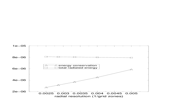
Figure 4: Convergence properties of a global energy conservation test. The difference between the initial and final Bondi mass converges in an almost second order way to the value given by the energy which is carried away by gravitational waves. The figure is taken from florian .

5 Summary

The article has dealt with presenting some concepts and applications in relativistic astrophysics of a particular class of finite difference numerical schemes based on Riemann solvers, specifically designed for nonlinear hyperbolic systems of conservation laws.

Such schemes have been discussed in the context of the general relativistic hydrodynamic equations. Nevertheless, the algorithms presented are general enough to be applicable to other hyperbolic systems such as the Einstein equations (when appropriately formulated, as e.g. in Friedrich’s conformal approach friedrich2 ; see also reula ). While this may not be strictly necessary for vacuum spacetimes, it may become relevant when dealing with nonvanishing stress-energy tensors.

The use of conservative algorithms based upon the characteristic structure of the hydrodynamic equations, developed during the last decade building on ideas first applied in Newtonian hydrodynamics, provides a robust methodology to obtain stable and accurate solutions even in the presence of discontinuities. This has become apparent since the early 1990s mim .

The knowledge of the wave structure of the equations is the essential building block in the construction of the so-called linearized Riemann solvers. The increasing use of these solvers in relativistic hydrodynamics has proved successful in handling complex flows, with high Lorentz factors and strong shocks, superseding more traditional methods based on artificial viscosity ibanez .

In the last part of the article we have discussed some astrophysical applications of such schemes, using the coupled system of the (characteristic) Einstein and hydrodynamic equations. Examples involving the gravitational collapse of supermassive stars and the evolution of relativistic compact stars have been presented.

References

- (1) M.W. Choptuik: Phys. Rev. Lett. 70, 9 (1993)
- (2) R. Gómez et al: Phys. Rev. Lett. 80, 3915 (1998)
- (3) A. Lichnerowicz: J. Math. Pure Appl. 23, 37 (1944)
- (4) Y. Choquet-Bruhat: In: Gravitation: An introduction to current research (John Wiley, New York 1962) pp.
- (5) R. Arnowitt, S. Deser, C.W. Misner: ‘The Dynamics of General Relativity’. In: Gravitation: An Introduction to Current Research (John Wiley, New York 1962) pp. 227-265
- (6) H. Friedrich, A.D. Rendall: Lect. Notes Phys. 540, 127 (2000)
- (7) O. Reula: Liv. Rev. Relativ. 1, 3 (1998)
- (8) M. Shibata, T. Nakamura: Phys. Rev. D 52, 5428 (1995)
- (9) T.W. Baumgarte, S.L. Shapiro: Phys. Rev. D 59, 024007 (1999)
- (10) E. Seidel, W.-M. Suen: J. Comput. Appl. Math. 109 (1999)
- (11) H. Bondi, M.J.G. van der Burg, A.W.K. Metzner: Proc. R. Soc. London, Sect. A 269, 21 (1962)
- (12) R.K. Sachs: Proc. R. Soc. London, Sect. A 270, 103 (1962)
- (13) R. Penrose: Phys. Rev. Lett. 10, 21 (1963)
- (14) J. Winicour: Liv. Rev. Relativ. 4, 3 (2001)
- (15) H. Friedrich: Proc. R. Soc. London A 375, 169 (1981)
- (16) P. Hübner: Phys. Rev. D 53, 701 (1996)
- (17) J. Frauendiener: Phys. Rev. D 58, 064003 (1998)
- (18) P. Hübner: Class. Quant. Grav. 18, 1421 (2001)
- (19) M.R. Dubal, R.A. d’Inverno, J.A. Vickers: Phys. Rev. D 58, 044019 (1998)
- (20) N. Bishop, R. Gómez, L. Lehner, M. Maharaj, J. Winicour: Phys. Rev. D 60, 024005 (1999)
- (21) P. Papadopoulos, J.A. Font: Phys. Rev. D 61, 024015 (2000)
- (22) P. Papadopoulos, J.A. Font: Phys. Rev. D 63, 044016 (2001)
- (23) F. Linke, J.A. Font, H.-Th. Janka, E. Müller, P. Papadopoulos: Astron. Astrophys., in press (2001), astro-ph/0103144
- (24) F. Siebel, J.A. Font, E. Müller, P. Papadopoulos: Characteristic numerical relativity applied to hydrodynamic studies of neutron stars. Proceedings of the 9th Marcel Grossmann Meeting. Ed. R. Ruffini. World Scientific (2001); gr-qc/0011096
- (25) J.A. Font: Liv. Rev. Relativ. 3, 2 (2000)
- (26) J.R. Wilson: Astrophys. J. 173, 431 (1972)
- (27) J.M. Martí, J.M. Ibáñez, J.A. Miralles: Phys. Rev. D 43 3794 (1991)
- (28) M.M May, R.H. White: Phys. Rev. D 141, 1232 (1966)
- (29) T. Nakamura: Prog. Theor. Phys. 65, 1876 (1981)
- (30) R.F. Stark, T. Piran: Phys. Rev. Lett. 55, 891 (1985)
- (31) H. Dimmelmeier, J.A. Font, E. Müller: astro-ph/0103088
- (32) T.W. Baumgarte, S.A. Hughes, S.L. Shapiro: Phys. Rev. D 60, 87501 (1999)
- (33) J.A. Font, M. Miller, W.-M. Suen, M. Tobias: Phys. Rev. D 61, 044011 (2000)
- (34) M. Alcubierre, B. Brügmann, T. Dramlitsch, J.A. Font, P. Papadopoulos, E. Seidel, N. Stergioulas, R. Takahashi: Phys. Rev. D 62, 044034 (2000)
- (35) N. Stergioulas, J.A. Font: Phys. Rev. Lett. 86, 1148 (2001)
- (36) J.A. Font, T. Goodale, S. Iyer, L. Rezolla, M. Miller, E. Seidel, W.M. Suen, M. Tobias, in preparation (2001)
- (37) G.J. Mathews, P. Marronetti, J.R. Wilson: Phys. Rev. D 58, 043003 (1998)
- (38) M. Shibata, Phys. Rev. D 60, 104052 (1999)
- (39) M. Shibata, K. Uryu: Phys. Rev. D 61, 064001 (2000)
- (40) M. Miller, W.M. Suen, M. Tobias: Phys. Rev. D 63, 121501 (2001)
- (41) K. Thorne: Gravitational Wave Astronomy. Proceedngs of the Yukawa Conference on Black Holes and Gravitational Waves: New Eyes in the 21st Century (1999)
- (42) Issacson, Welling y Winicour, J. Math. Phys., 24, 1824 (1983)
- (43) R.J. LeVeque: Numerical Methods for Conservation Laws. Birkhäuser-Verlag (1990)
- (44) E.F. Toro: Riemann Solvers and Numerical Methods for Fluid Dynamics. Springer-Verlag, Berlin, Heidelberg (1997)
- (45) C. Hirsch: Numerical Computation of Internal and External Flows. Wiley (1988)
- (46) C.B. Laney: Computational gasdynamics, Cambridge University Press (1998)
- (47) J.M. Ibáñez, J.M. Martí: J. Comput. Appl. Math. 109, 173 (1999)
- (48) J.M. Martí, E. Müller: Liv. Rev. Relativ. 2, 1 (1999)
- (49) J. von Neumann, R.D. Richtmyer: J. Appl. Phys. 21, 232 (1950)
- (50) M.L. Norman, K-H. A. Winkler: In Astrophysical Radiation Hydrodynamics. Eds. M.L. Norman, K-H. A. Winkler, Reidel Publishing Company, 449 (1986)
- (51) S. Siegler, H. Riffert: Astrophys. J. 531, 1053 (2000)
- (52) A.M. Anile: Relativistic Fluids and Magneto-fluids, Cambridge University Press, Cambridge, England (1989)
- (53) J.A. Font, J.M. Ibáñez, J.M. Martí, A. Marquina: Astron. Astrophys. 282, 304 (1994)
- (54) F. Eulderink, G. Mellema: Astron. Astrophys. Suppl. Ser. 110, 587 (1995)
- (55) S.A.E.G. Falle, S.S. Komissarov: Mon. Not. R. Astron. Soc. 278, 586 (1996)
- (56) F. Banyuls, J.A. Font, J.M. Ibáñez, J.M. Martí, J.A. Miralles: Astrophys. J. 476, 221 (1997)
- (57) L. Wen, A. Panaitescu, P. Laguna: Astrophys. J. 486, 919 (1997)
- (58) J.M. Ibáñez, M.A. Aloy, J.A. Font, J.M. Martí, J.A. Miralles, J.A. Pons: Riemann solvers in general relativistic hydrodynamics. In E.F. Toro ed. Godunov Methods: Theory and Applications. In press (2001)
- (59) P.D. Lax, B. Wendroff: Comm. Pure Appl. Math. 13, 217 (1960)
- (60) P.D. Lax: Regional Conference Series Lectures in Applied Math. 11, SIAM, Philadelphia (1972)
- (61) R.D. Richtmyer, K.W. Morton: Difference Methods for Initial-Value Problems. Wiley-Interscience, New York (1967)
- (62) A. Harten: SIAM J. Numer. Anal. 21, 1 (1984)
- (63) S.K. Godunov: Mat. Sb. 47, 271 (1959) in Russian
- (64) J.M. Martí, E. Müller: J. Fluid Mech. 258, 317 (1994)
- (65) J. Pons, J.M. Martí, E. Müller: J. Fluid Mech. 422, 125 (2000)
- (66) A. Harten, P.D. Lax, B. van Leer: SIAM Review 25, 35 (1983)
- (67) B. Einfeldt: SIAM J. Num. Anal. 25, 294 (1988)
- (68) P.L. Roe: J. Comput. Phys. 43, 357 (1981)
- (69) B. van Leer: J. Comput. Phys. 32, 101 (1979)
- (70) P. Colella, P.R. Woodward: J. Comput. Phys. 54, 174 (1984)
- (71) A. Harten, B. Engquist, S. Osher, S.R. Chakrabarthy: J. Comput. Phys. 71, 231 (1987)
- (72) R.J. LeVeque: Nonlinear Conservation Laws and Finite Volume Methods. In Computational Methods for Astrophysical Fluid Flow. Saas-Fee Advanced Course 27. Lecture Notes 1997. Springer-Verlag, 1 (1998)
- (73) R. Donat, J.A. Font, J.M. Ibáñez, A. Marquina: J. Comput. Phys. 146, 58 (1998)
- (74) M.J. Rees: In Black Holes and Relativistic Stars, University of Chicago Press, Chicago (1998)
- (75) J. Kormendy: astro-ph (2000)
- (76) S. Chandrasekhar: Astrophys. J. 140, 417 (1964)
- (77) W.F. Fowler: Rev. Mod. Phys. 36, 545 (1964)
- (78) G.M. Fuller, X. Shi: Astrophys. J. 502, L5 (1998)
- (79) T. Zwerger, E. Müller: Astron. Astrophys. 320, 209 (1997)
- (80) R. Gómez, P. Papadopoulos, J. Winicour: J. Math. Phys. 35, 4184 (1994)