The runaway instability of thick discs around black holes.
I. The constant angular momentum case

Abstract

We present results from a numerical study of the runaway instability of thick discs around black holes. This instability is an important issue for most models of cosmic gamma-ray bursts, where the central engine responsible for the initial energy release is such a system consisting of a thick disc surrounding a black hole. We have carried out a comprehensive number of time-dependent simulations aimed at exploring the appearance of the instability. Our study has been performed using a fully relativistic hydrodynamics code. The general relativistic hydrodynamic equations are formulated as a hyperbolic flux-conservative system and solved using a suitable Godunov-type scheme. We build a series of constant angular momentum discs around a Schwarzschild black hole. Furthermore, the self-gravity of the disc is neglected and the evolution of the central black hole is assumed to be that of a sequence of exact Schwarzschild black holes of varying mass. The black hole mass increase is thus determined by the mass accretion rate across the event horizon. In agreement with previous studies based on stationary models, we find that by allowing the mass of the black hole to grow the disc becomes unstable. Our hydrodynamical simulations show that for all disc-to-hole mass ratios considered (between 1 and 0.05), the runaway instability appears very fast on a dynamical timescale of a few orbital periods, typically a few 10 ms and never exceeding 1 s for our particular choice of the mass of the black hole ($2.5\ \mathrm{M_{\odot}}$) and a large range of mass fluxes ($\dot{m}\ga 10^{-3}\ \mathrm{M_{\odot}/s}$). The implications of our results in the context of gamma-ray bursts are briefly discussed.

1 Introduction

Table 1: Summary of representative results concerning the runaway instability on stationary models of thick discs around black holes.

Reference	Framework	Angular momentum	BH rotation	Disc self-gravity	Results
Abramowicz et al. (1983)	Pseudo-Newt.	$l=\mathrm{constant}$	no	approximate	unstable1
Wilson (1984)	GR	$l=\mathrm{constant}$	yes	neglected	stable
Khanna & Chakrabarti (1992)	Pseudo-Newt.	$l=\mathrm{constant}$	yes	approximate	unstable
Nishida et al. (1996)	GR	$l=\mathrm{constant}$	yes	exact	unstable2
Daigne & Mochkovitch (1997)	Pseudo-Newt.	$l\propto\varpi^{\alpha}$, $0\leq\alpha\leq 0.5$	no	neglected	stable3
Abramowicz et al. (1998)	GR	$l\propto\varpi^{\alpha}$, $0\leq\alpha\leq 0.5$	yes	neglected	stable4
Masuda et al. (1998)	Pseudo-Newt.	$l\propto\varpi^{\alpha}$, $\alpha=0.2$	no	exact	unstable5
Lu et al. (2000)	Pseudo-Newt.	$l\propto\varpi^{\alpha}$, $0\leq\alpha\leq 0.5$	no	neglected	stable6

Notes :

1 for a large range of disc-to-hole mass ratio and disc inner radius.

2 study made for only four intial models.

3 The mass of the black hole is $2.44\ \mathrm{M}_{\odot}$. The mass of the disc is $0.36\ \mathrm{M}_{\odot}$. The system is stable for $\alpha\geq\alpha_{\mathrm{cr}}$ with $\alpha_{\mathrm{cr}}\sim 0.1$.

4 Same parameters as Daigne & Mochkovitch (1997). The critical value $\alpha_{\mathrm{cr}}$ decreases when the black hole rotation increases.

5 Same parameters as Daigne & Mochkovitch (1997). The system becomes unstable for large transfer of mass only.

6 Same conclusion as Daigne & Mochkovitch (1997) for a completely different range of masses (massive black hole of mass $10^{6}\ \mathrm{M}_{\odot}$).

Thick accretion discs are probably present in many astrophysical objects, e.g. quasars and other active galactic nuclei, some X-ray binaries and microquasars, and the central engine of gamma-ray bursts (GRBs hereafter). They have been studied in great detail by many authors (see e.g. Rees (1984) and references therein). In particular, it is well known that in a system formed by a black hole surrounded by a thick disc, the gas flows in an effective (gravitational plus centrifugal) potential, whose structure is comparable with that of a close binary. The Roche torus surrounding the black hole has a cusp-like inner edge located at the Lagrange point $\mathrm{L}_{1}$ where mass transfer driven by the radial pressure gradient is possible (Kozlowski et al. 1978).

The so-called runaway instability of such systems was first discovered by Abramowicz et al. (1983). The underlying mechanism is the following: due to accretion of material from the disc, the mass of the black hole increases and the gravitational field of the system changes. Therefore, an accretion disc can never reach a completely steady state. Starting from an initial disc filling its Roche lobe so that mass transfer is possible through the cusp located at the $\mathrm{L}_{1}$ Lagrange point, two evolutions are feasible when the mass of the black hole increases: (i) either the cusp moves inwards towards the black hole, which slows down the mass transfer, resulting in a stable situation, or (ii) the cusp moves deeper inside the disc material. In this case the mass transfer speeds up, leading to the runaway instability.

In their first study, Abramowicz et al. (1983) analyzed the effect of the mass transfer under many simplifying assumptions (a pseudo-Newtonian potential for the black hole (Paczyński & Wiita 1980), constant angular momentum in the disc, and approximate treatment of the disc self-gravity). These authors found that the runaway instability occurs for a large range of parameters such as the disc-to-hole mass ratio and the location of the disc inner radius. More detailed studies followed, whose main conclusions are summarized in Table 1. Notice that all these studies are based on stationary models in which a fraction of the mass and angular momentum of an initial disc filling its Roche lobe is transfered to the black hole, and the new gravitational field is used to compute the new position of the cusp, which controls whether the runaway instability occurs or not. The conclusions of these studies have yet to be confirmed on a dynamical framework.

From Table 1 one sees that (i) taking into account the self-gravity of the disc seems to favor the instability (Khanna & Chakrabarti 1992; Nishida et al. 1996; Masuda et al. 1998); (ii) the rotation of the black hole has a stabilizing effect (Wilson 1984; Abramowicz et al. 1998); (iii) taking into account a non-constant distribution of the angular momentum (increasing outwards) has a strong stabilizing effect (Daigne & Mochkovitch 1997; Abramowicz et al. 1998); (iv) using a fully relativistic potential instead of a pseudo-Newtonian potential for the black hole seems to act in the direction of favoring the instability (Nishida et al. 1996). It also becomes evident from Table 1 that there is not still a final consensus about the very existence of the instability. In the fully relativistic study of Nishida et al. (1996), it was shown that the runaway instability occurs when the angular momentum is constant in the disc. However, the work of Daigne & Mochkovitch (1997) showed the stabilizing effect of a distribution of angular momentum in the disc increasing outwards. It is worth pointing out that the complete calculation in this setup, i.e., in general relativity and including self-gravity and a rotating black hole, is extremely complex and has not been done yet.

The consequences of the runaway instability could be very important in many cases. First because this is a purely dynamical effect, so that its time-scale is extremely short (only a few ms for a stellar mass black hole). This means that this instability should happen before any other processes (like the viscous transport of angular momentum) could play a role. Secondly, because the radial mass transfer is supposed to diverge, so that the thick disc could, in principle, be completely destroyed.

In particular, Nishida et al. (1996) pointed out that the runaway instability could be a severe problem for most current models of GRBs. These models usually assume that the central engine is such a system consisting of a black hole and a thick disc, either formed at the late stages of the coalescence of two neutron stars (Kluzniak & Lee 1998; Ruffert & Janka 1999; Shibata & Uryū 2000) or after the gravitational collapse of a massive star (Paczynski 1986; Woosley 1993). Notice that in the latter case, the situation is somewhat more complicated because the mass of the disc increases with time, as long as the collapse proceeds (MacFadyen & Woosley 1999; Aloy et al. 2000). The energy which can be extracted from this system comes from two reservoirs: the energy released by the accretion of disc material on to the black hole and the rotational energy of the black hole itself, which can be extracted via the Blandford-Znajek mechanism (Blandford & Znajek 1977). This amount of energy (a few $10^{53}$–$10^{54}$ erg depending on the disc mass and the black hole rotation and mass) is sufficient to power a GRB if the energy released can be eventually converted into $\gamma$-rays with a large efficiency of about a few percent. This number, however, depends strongly on the central engine model and on the expected beaming of the outflow, which is currently very poorly constrained. Such conversion cannot be done close to the source, the luminosity considered here being many orders of magnitude larger than the Eddington luminosity of the system. The energy is first injected into a very optically thick wind. This wind is accelerated via some mechanism which is still unknown but which involves probably MHD processes (Thompson 1994; Meszaros & Rees 1997b) and becomes eventually relativistic. The existence of such a relativistic wind has been directly inferred from the observations of radio scintillation in GRB 970508 (Waxman et al. 1998) and is also needed to solve the so-called compactness problem and avoid photon-photon annihilation along the line of sight. Averaged Lorentz factors larger than 100 are required (Baring & Harding 1997; Lithwick & Sari 2001). The observed emission is produced at large distances from the source ($r>10^{11}$–$10^{12}\ \mathrm{cm}$), probably via the formation of shock waves, either within the wind itself (internal shock model, proposed for the prompt $\gamma$-ray emission, (Rees & Meszaros 1994; Kobayashi et al. 1997; Daigne & Mochkovitch 1998)) or caused by the deceleration of the wind by the external medium (external shock model, which reproduces correctly the afterglow emission (Meszaros & Rees 1997a; Sari et al. 1998)).

The above general scenario clearly presupposes that the black hole plus thick disc system is stable enough to survive for a few seconds (in particular, the internal shock model implies that the duration of the energy release by the source has a duration comparable with the observed duration of the GRB). However, if the runaway instability would occur, the disc would fall into the hole in just a few milliseconds!

In order to establish the nature of instabilities in accretion flows one must rely upon highly accurate, time-dependent, nonlinear numerical simulations in black hole spacetimes. These simulations are scarce and they have been mostly performed using a Newtonian or a pseudo-Newtonian potential which mimics the existence of an “event horizon” (Paczyński & Wiita 1980) (see Eggum et al. (1988); Papaloizou & Szuszkiewicz (1994); Igumenshchev et al. (1996) for simulations in the context of thick discs). Concerning relativistic simulations Wilson (1972) was the first to study numerically the time-dependent accretion of matter on to a rotating black hole. His simulations showed the formation of thick accretion discs. In a subsequent work Hawley et al. (1984a, b) studied the evolution and development of nonlinear instabilities in pressure-supported accretion discs formed as a consequence of the spiraling infall of fluid with some amount of angular momentum. Their constant angular momentum initial models were computed following the analytic theory of relativistic discs developed by Kozlowski et al. (1978). The code developed by Hawley et al. (1984a, b) was capable of keeping stable discs in equilibrium as well as of following the fate of initially unstable models. Yokosawa (1995) studied the structure and dynamics of relativistic accretion discs and the transport of energy and angular momentum in magnetohydrodynamical accretion on to a rotating black hole. More recently, Igumenshchev & Beloborodov (1997) performed a similar study as Hawley et al. (1984a, b), including the rotating black hole case and using improved numerical methods based on Riemann solvers. They found that the structure of the innermost part of the disc depends strongly on the black hole spin and, at the same time, they were able to confirm numerically the expected analytic dependence of the mass accretion rate with the gravitational energy gap at the cusp of the torus.

A time-dependent and fully relativistic study of the runaway stability has not yet been presented in the literature. Masuda & Eriguchi (1997) performed a time-dependent simulation in a pseudo-Newtonian framework, using an SPH method so that the self-gravity was taken into account. Our work aims at providing the first relativistic study. We have investigated the likelihood of the instability in thick discs of constant angular momentum. In this first investigation we present results for a Schwarzschild black hole. The rotating case and the inclusion of accretion discs with a distribution of angular momentum increasing outwards will be presented elsewhere. Our simulations are performed in a fully relativistic framework, using a 3+1 conservative formulation of the hydrodynamic equations on a curved background (Banyuls et al. 1997) and employing Godunov-type numerical methods for their solution (see e.g. Font (2000) and references therein). As in the work of Hawley et al. (1984a, b) and Igumenshchev & Beloborodov (1997) we neglect viscous and radiative processes assuming that the flow is isentropic. This is justified as we are only interested in phenomena occurring on a dynamical timescale. Furthermore, as a major simplification of the computational burden, we neglect the self-gravity of the disc. The spacetime dynamics has hence been treated in a simple way, assuming that the background spacetime metric is nothing but a sequence of stationary exact black hole solutions (Schwarzschild or Kerr) of the Einstein equations, whose dynamics is governed by the increase of the black hole mass (and angular momentum). Such growth is controlled only by the rate at which the mass accretes on to the hole. We are aware that a fully consistent approach to study the problem would imply solving the coupled system of Einstein and hydrodynamic equations in three-dimensions. This seems still a daunting task despite some major recent progress on numerically stable integrations of the Einstein equations (see, e.g., Alcubierre et al. (2000); Font et al. (2001) and references therein). We believe that, as a first step, our approach is justified and can provide some insight on the problem.

The paper is organized as follows: Section 2 reviews briefly the theory of stationary, relativistic accretion discs of constant angular momentum. In Section 3 we introduce the equations of general relativistic hydrodynamics in the way they are used in our code. The numerical schemes we use to solve those equations, as well as other relevant aspects of our numerical code are described in Section 4. In Section 5 we test the capability of the code in keeping numerically the equilibrium of stationary models in time-dependent simulations. The main results of the paper are presented in Section 6 which contains the simulations of the runaway instability. Finally, Section 7 presents a summary of our investigation.

Unless explicitly stated we are using geometrized units ($G=c=1$) throughout the paper. Greek (Latin) indices run from 0 to 3 (1 to 3). We also use the signature -+++. Usual cgs units are obtained by using the gravitational radius of the black hole, $r_{\mathrm{g}}=GM_{\mathrm{BH}}/c^{2}$, as unit of length. Although this paper is only concerned with the Schwarzschild case we present all expressions for the most general setup of a Kerr black hole in order to refer to them in the forthcoming papers of this series. The code is already written for the Kerr metric and the results here presented have been obtained by just setting to zero the black hole angular momentum parameter.

2 Stationary models of thick accretion discs

The theory of stationary, relativistic thick discs (or tori) of constant angular momentum was first derived by Fishbone & Moncrief (1976) for isentropic discs and by Kozlowski et al. (1978) for discs obeying a barotropic equation of state (EoS). Although this theory is by now well-established and has been presented in great detail elsewhere, we have chosen to include here the relevant aspects and definitions in order to facilitate the self-consistency of the paper.

2.1 Definitions

2.1.1 Assumptions

In order to build up constant angular momentum configurations for a given metric we assume a number of conditions. Firstly, the torus is stationary and axially symmetric. We adopt the standard spherical coordinates $(t,r,\theta,\phi)$ in which the metric coefficients neither depend on the time coordinate $t$ (stationarity) or on the azimuthal coordinate $\phi$ (axisymmetry). The line element of the spacetime is given by

$$ds^{2}=g_{tt}dt^{2}+2g_{t\phi}dtd\phi+g_{\phi\phi}d\phi^{2}+g_{rr}dr^{2}+g_{\theta\theta}d\theta^{2}\ .$$ (1)

We adopt the following convention: the angular momentum of the black hole is positive and the matter of the disc rotates in the positive (negative) direction of $\phi$ for a prograde (retrograde) disc. We define the following quantity which is a relativistic generalization of the “distance to the axis”:

$$\varpi^{2}=g_{t\phi}^{2}-g_{tt}g_{\phi\phi},$$ (2)

which in the Newtonian limit is simply $\varpi=r\sin\theta$.

The EoS of the fluid is assumed to be barotropic, so that $p=p(e)$ where $p$ is the pressure and $e$ is the total energy density. We define $\rho$ as the rest mass density, $w=e+P$ as the enthalpy and $h=w/\rho$ as the specific enthalpy. The four velocity of the fluid is $u^{\mu}=(u^{t},0,0,u^{\phi})$ with the normalization condition $u^{2}=u_{\mu}u^{\mu}=-1$.

2.1.2 Von Zeipel’s cylinders

The Lagrangian angular momentum (angular momentum per unit inertial mass) and the angular velocity are respectively defined by

$$l=-\frac{u_{\phi}}{u_{t}}$$ (3)

and

$$\Omega=\frac{u^{\phi}}{u^{t}}\ .$$ (4)

From $u_{\mu}=g_{\mu\nu}u^{\nu}$ it follows that

$$l=-\frac{g_{t\phi}+g_{\phi\phi}\Omega}{g_{tt}+g_{t\phi}\Omega}\ \mathrm{and}\ \Omega=-\frac{g_{t\phi}+g_{tt}l}{g_{\phi\phi}+g_{t\phi}l}\ .$$ (5)

For a barotropic EoS, the equi-$l$ and equi-$\Omega$ surfaces coincide and they are called the von Zeipel’s cylinders. Their cylinder-like topology has been proved by Abramowicz (1974). If the metric is known, Eq. (5) allows to construct the von Zeipel’s cylinder defined by $l_{0}$ and $\Omega_{0}$ by solving the following equation

$$g_{tt}l_{0}+g_{t\phi}\left(1+\Omega_{0}l_{0}\right)+g_{\phi\phi}\Omega_{0}=0\ .$$ (6)

In particular, if the distribution of the angular momentum $l=l_{\mathrm{eq}}(r)$ is given in the equatorial plane $\theta=\pi/2$, then the corresponding distribution of the angular velocity in the equatorial plane is given by

$$\Omega=\Omega_{\mathrm{eq}}(r)=-\frac{g_{t\phi}(r,\pi/2)+g_{tt}(r,\pi/2)l(r)}{g_{\phi\phi}(r,\pi/2)+g_{t\phi}(r,\pi/2)l(r)}\ .$$ (7)

The equation of the von Zeipel’s cylinder intersecting the equatorial plane at a given radial point $r=r_{0}$ is given by Eq. (6) so that

$$l^{2}(r_{0})\left[g_{tt}(r,\theta)g_{t\phi}(r_{0},\pi/2)-g_{t\phi}(r,\theta)g_{tt}(r_{0},\pi/2)\right]$$

$$+l(r_{0})\left[g_{tt}(r,\theta)g_{\phi\phi}(r_{0},\pi/2)-g_{\phi\phi}(r,\theta)g_{tt}(r_{0},\pi/2)\right]$$

$$+\left[g_{t\phi}(r,\theta)g_{\phi\phi}(r_{0},\pi/2)-g_{\phi\phi}(r,\theta)g_{t\phi}(r_{0},\pi/2)\right] = 0\ .$$

Notice that in the case of the Schwarzschild metric, $g_{t\phi}=0$, and this equation reduces to

$$g_{tt}(r,\theta)g_{\phi\phi}(r_{0},\pi/2)-g_{\phi\phi}(r,\theta)g_{tt}(r_{0},\pi/2)=0$$ (9)

which is independent of the distribution of angular momentum.

2.1.3 Equipotentials

The dynamics of the gas flow is governed by the relativistic Euler equation, whose integral form is

$$W-W_{\mathrm{in}}=\ln{(-u_{t})}-\ln{(-\left.u_{t}\right._{\mathrm{in}})}-\int_{l_{\mathrm{in}}}^{l}\frac{\Omega dl}{1-\Omega l}\ .$$ (10)

The subscript “$\mathrm{in}$” refers to the inner edge (in the equatorial plane) of the disc, where the pressure vanishes. The quantity $W$ is defined by

$$W-W_{\mathrm{in}}=-\int_{0}^{p}\frac{dp}{w}\ .$$ (11)

In the Newtonian limit, the quantity $W$ is the total (centrifugal plus gravitational) potential and Eq. (11) is the integral form of the equation of hydrostatic equilibrium. If the spacetime metric is known and if the distribution of angular momentum in the equatorial plane is given, so that the von Zeipel’s cylinders have been computed, providing us with the value of $l$ and $\Omega$ at any given point within the disc, then the equipotentials surfaces $W(r,\theta)$ are easily computed from Eq. (10) taking into account that $u_{t}$ can be expressed (from the 4-velocity normalization condition $u^{2}=-1$) as a function of $l$ by

$$-u_{t}=\sqrt{\frac{\varpi^{2}}{g_{tt}l^{2}+2g_{t\phi}l+g_{\phi\phi}}}\ .$$ (12)

2.1.4 Construction of a thick disc

In order to build a system consisting of a black hole surrounded by a thick disc we need several parameters: the mass $M$ and the specific angular momentum $a=J/M$ of the black hole, the distribution of the angular momentum of the disc in the equatorial plane $l_{\mathrm{eq}}(r)$, the inner radius of the disc $r_{\mathrm{in}}$ and the EoS of the fluid material of the disc. The procedure is then the following:

1. Compute the metric coefficients in a Kerr background with free parameters $a$ and $M$ (these coefficients are given in the next Section).

2. From the distribution of the angular momentum in the equatorial plane, solve Eq. (6) to have the distribution of angular momentum $l(r,\theta)$. Then the corresponding distribution $u_{\mathrm{t}}(r,\theta)$ can be evaluated from Eq. (12).

3. From the value of the inner radius $r_{\mathrm{in}}$, compute the corresponding value of the angular momentum $l_{\mathrm{in}}=l_{\mathrm{eq}}(r_{\mathrm{in}})$. Then the function

   $$F(r,\theta)=\int_{l_{\mathrm{in}}}^{l}\frac{\Omega dl}{1-\Omega l}$$ (13)

   can be evaluated.

4. Compute the potential

   $$W(r,\theta)-W_{\mathrm{in}}=\ln{\left(-u_{t}(r,\theta)\right)}-\ln{\left(-\left.u_{t}\right._{\mathrm{in}}\right)}-F(r,\theta)\ .$$

   The constant $W_{\mathrm{in}}$ is fixed by the convention that $\lim_{r\to+\infty}W(r,\theta)=0$.

5. Compute all hydrodynamical quantities ($p$, $\rho$, $e$, $w$, etc) from the EoS and Eq. (11). In the following , we will only consider the particular case of isentropic fluids where

   $$\int_{0}^{p}\frac{dp}{w}=\ln{\frac{h}{h_{\mathrm{in}}}}\ .$$ (14)

If the self-gravity of the disc is neglected, the procedure stops here. Otherwise, from the distribution of matter-energy we have computed, we need to solve the Einstein field equations to evaluate the new metric coefficients $g_{\mu\nu}$. Then the procedure starts again at step 2. Such cycles are repeated until convergence.

Once a disc has been built, one can estimate its mass with the expression

$$m=\int\!\!\!\!\int\!\!\!\!\int\!\left(T^{\phi}_{\phi}+T^{r}_{r}+T^{\theta}_{\theta}-T^{t}_{t}\right)\sqrt{-g}\ dV\ ,$$ (15)

where $T^{\mu\nu}$ is the stress-energy tensor which, in the case of a perfect fluid is defined by $T^{\mu\nu}=\rho hu^{\mu}u^{\nu}+pg^{\mu\nu}$. In all the models we will consider in the following, we have $p\ll e$ so that the mass of the disc can be accurately approximated by the rest-mass

$$m \simeq \int\!\!\!\!\int\!\!\!\!\int\!\!\rho\left(u_{\phi}u^{\phi}-u_{t}u^{t}\right)\sqrt{-g}\ dV$$ (16)

$$\simeq \int\!\!\!\!\int\!\!\!\!\int\!\!\frac{1+\Omega l}{1-\Omega l}\rho\sqrt{-g}\ dV\ .$$

Figure 1: The von Zeipel’s cylinders for the Schwarzschild metric. The critical cylinder (thick line) has a cusp located at $r=3$ in the equatorial plane.

2.2 Constant angular momentum thick discs orbiting a Schwarzschild black hole

In this subsection we describe in detail the particular case we have considered for the time-dependent simulations of this paper: the black hole is non-rotating (a Schwarzschild black hole), the self-gravity of the disc is neglected, the angular momentum $l$ is constant and the disc obeys a polytropic EoS with

$$P=\kappa\rho^{\gamma},$$ (17)

with $\kappa$ being the polytropic constant and $\gamma$ the adiabatic exponent. For commodity, we further assume that the mass of the black hole is equal to unity. The metric coefficients are given by

$$g_{tt} = -\left(1-\frac{2}{r}\right),$$ (18)

$$g_{t\phi} = 0,$$ (19)

$$g_{\phi\phi} = r^{2}\sin^{2}\theta,$$ (20)

and the distance to the axis is simply $\varpi^{2}=r(r-2)\sin^{2}\theta$. As the black hole is non-rotating, we also consider only positive values of the angular momentum (prograde discs).

The von Zeipel’s cylinders are independent of $l$. Using Eq. (9), the cylinder intersecting the equatorial plane at $r=r_{0}$ is given by

$$(r_{0}-2)r^{3}\sin^{2}\theta-r_{0}^{3}(r-2)=0\ .$$ (21)

The result is shown in Fig. 1. Notice the cusp located at $r=3$ in the equatorial plane (thick line).

Since the angular momentum $l$ is constant, the function $F(r,\theta)$ vanishes. Using Eq. (12), the component $u_{t}$ of the 4-velocity is given by

$$-u_{t}=r\sin{\theta}\sqrt{\frac{r-2}{r^{3}\sin^{2}\theta-(r-2)l^{2}}}$$ (22)

and the potential $W$ reads

$$W(r,\theta)=\frac{1}{2}\ln{\frac{r^{2}(r-2)\sin^{2}\theta}{r^{3}\sin^{2}\theta-l^{2}(r-2)}},$$ (23)

where we have used the condition $W(r,\theta)\to 0$ for $r\to+\infty$ to eliminate $r_{\mathrm{in}}$.

We describe now the equipotentials which are either closed ($W<0$) or open ($W>0$). The marginal case $W=0$ is closed at infinity. The geometry of the equipotentials is fixed by the value of $l$. We impose that $W(r)$ is defined everywhere outside the horizon in the equatorial plane, i.e. that the term $r^{3}-l^{2}(r-2)$ never vanishes. Then $l<l_{\mathrm{max}}=3\sqrt{3}\simeq 5.20$.

Table 2: The possible equipotential configurations for a Schwarzschild black hole and a constant angular momentum disc.

Angular momentum	$r_{\mathrm{cusp}}$	$W_{\mathrm{cusp}}$	$r_{\mathrm{center}}$	$W_{\mathrm{center}}$	Comments
$l<l_{\mathrm{ms}}\simeq 3.67$					No cusp. No center. Disc infinite.
$l=l_{\mathrm{ms}}\simeq 3.67$	$r_{\mathrm{cusp}}=r_{\mathrm{ms}}=6$	$<0$	$r_{\mathrm{center}}=r_{\mathrm{ms}}=6$	$<0$	Cusp = center. Disc infinite.
$l_{\mathrm{ms}}<l<l_{\mathrm{mb}}$	$r_{\mathrm{mb}}<r_{\mathrm{cusp}}<r_{\mathrm{ms}}$	$<0$	$r_{\mathrm{center}}>r_{\mathrm{ms}}$	$<0$	Cusp. Center. Disc closed.
$l=l_{\mathrm{mb}}=4$	$r_{\mathrm{cusp}}=r_{\mathrm{mb}}=4$	$0$	$r_{\mathrm{center}}\simeq 10.47$	$<0$	Cusp. Center. Disc closed at infinity.
$l_{\mathrm{mb}}<l<l_{\mathrm{max}}$	$r_{\mathrm{cusp}}<r_{\mathrm{mb}}$	$>0$	$r_{\mathrm{center}}\ga 10.47$	$<0$	Cusp. Center. Disc infinite∗.
$l=l_{\mathrm{max}}\simeq 5.20$	$r_{\mathrm{cusp}}=3$	$+\infty$	$r_{\mathrm{center}}\simeq 22.39$	$<0$	Cusp marginally defined. Center. Disc infinite∗.

^∗ Some closed equipotentials are still present around the center.

It can be easily shown that the presence of a cusp in the equatorial plane is related to the solutions of

$$l_{\mathrm{K}}(r)=l\ ,$$ (24)

where $l_{\mathrm{K}}(r)$ is the Keplerian angular momentum of a particle located at a radius $r$ in the equatorial plane. It is given by

$$l_{\mathrm{K}}(r)=\frac{r\sqrt{r}}{r-2}\ .$$ (25)

Two useful radii can be defined, the radius of the last (marginally) stable orbit $r_{\mathrm{ms}}=6$ (corresponding to the minimum of $l_{\mathrm{K}}(r)$), and the radius of the last (marginally) bound orbit $r_{\mathrm{mb}}=4$. The corresponding values of $l_{\mathrm{K}}$ are $l_{\mathrm{ms}}=\frac{3\sqrt{6}}{2}\simeq 3.67$ and $l_{\mathrm{mb}}=4$. The properties of $W(r,\theta)$ are given in Table 2 for the different possible values of $l$. The corresponding equipotentials are drawn in Fig. 2 (right panel). The angular momentum and potential in the equatorial plane are also drawn on the left panel of Fig. 2. It is clear that the most interesting case is case (3) where $l_{\mathrm{ms}}<l<l_{\mathrm{mb}}$ so that there exist a cusp, a center, and the equipotential of the cusp is closed. From Eq. (17) and Eq. (14) we have indeed

$$W-W_{\mathrm{in}}=-\ln{h}=-\ln{\left(1+\frac{\gamma}{\gamma-1}\kappa\rho^{\gamma-1}\right)},$$ (26)

so that the matter can fill only the part where $W\leq W_{\mathrm{in}}$. The density and the pressure are then easily determined from $h$:

$$h = e^{W_{\mathrm{in}}-W},$$ (27)

$$\rho = \left(\frac{\gamma-1}{\gamma}\frac{e^{W_{\mathrm{in}}-W}-1}{\kappa}\right)^{\frac{1}{\gamma-1}},$$ (28)

$$P = \kappa\left(\frac{\gamma-1}{\gamma}\frac{e^{W_{\mathrm{in}}-W}-1}{\kappa}\right)^{\frac{\gamma}{\gamma-1}}.$$ (29)

It is then possible to adjust the value of $l$ and $r_{\mathrm{in}}$ to fix the mass of the disc, which is given by

$$m\simeq 2\pi\int\!\!\!\!\int\!\!\rho\frac{r^{3}\sin^{2}\theta+(r-2)l^{2}}{r^{3}\sin^{2}\theta-(r-2)l^{2}}r^{2}\sin\theta d\theta dr\ .$$ (30)

If one imposes the condition that the disc is exactly filling its Roche lobe, the inner radius $r_{\mathrm{in}}=r_{\mathrm{cusp}}$ is fixed. Otherwise, instead of specifying $r_{\mathrm{in}}$, one could prefer another parameter, such as the potential barrier (energy gap) at the inner edge defined as

$$\Delta W_{\mathrm{in}}=W_{\mathrm{in}}-W_{\mathrm{cusp}}\ .$$ (31)

The case $\Delta W_{\mathrm{in}}<0$ corresponds to a disc inside its Roche lobe. No mass transfer is possible. The case $\Delta W_{\mathrm{in}}>0$ corresponds to a disc overflowing its Roche lobe: mass transfer is possible at the cusp. An analytic estimation for the mass flux (flux of rest mass density) was derived by Kozlowski et al. (1978) for this last case, showing the following dependence:

$$\dot{m}\propto\Delta W_{\mathrm{in}}^{\frac{\gamma}{\gamma-1}}.$$ (32)

Figure 2: Constant angular momentum thick disc orbiting a Schwarzschild black hole: Equipotentials for different values of $l$ (right column). The thick line corresponds to the equipotential of the cusp and a thick dot marks the center. The physically interesting case (corresponding to a thick torus) is case (3).

Figure 3: continued

Constant angular momentum thick disc orbiting a Schwarzschild black hole: Equipotentials for different values of $l$ (right column). The thick line corresponds to the equipotential of the cusp and a thick dot marks the center.

3 Hydrodynamic equations in a Kerr background

Our purpose is to evolve in time the initial data described in the previous Section. In order to do so we present in this Section the formulation of the general relativistic hydrodynamic equations in the form they have been implemented in our numerical code.

Using Boyer-Lindquist $(t,r,\theta,\phi)$ coordinates, the Kerr line element, $ds^{2}=g_{\mu\nu}dx^{\mu}dx^{\nu}$, reads

$$ds^{2} = -{{\Delta-a^{2}\sin^{2}\theta}\over{\varrho^{2}}}dt^{2}-2a{{2Mr\sin^{2}\theta}\over{\varrho^{2}}}dtd\phi$$ (33)

$$+ {{\varrho^{2}}\over{\Delta}}dr^{2}+\varrho^{2}d\theta^{2}+{{\Sigma}\over{\varrho^{2}}}\sin^{2}\theta d\phi^{2},$$

with the definitions:

$$\Delta \equiv r^{2}-2Mr+a^{2},$$ (34)

$$\varrho^{2} \equiv r^{2}+a^{2}\cos^{2}\theta,$$ (35)

$$\Sigma \equiv (r^{2}+a^{2})^{2}-a^{2}\Delta\sin^{2}\theta,$$ (36)

where $M$ is the mass of the black hole and $a$ is the black hole angular momentum per unit mass ($J/M$). Notice that the geometrical factor $\varrho$ has not to be confused with the rest-mass density of the fluid, $\rho$. The above metric, Eq. (33), describes the spacetime exterior to a rotating and non-charged black hole. The metric has a coordinate singularity at the roots of the equation $\Delta=0$, which correspond to the horizons of a rotating black hole, $r=r_{\pm}=M\pm(M^{2}-a^{2})^{1/2}$. The “distance to the rotation axis” introduced in the previous Section is given by $\varpi^{2}=g_{t\phi}^{2}-g_{tt}g_{\phi\phi}=\Delta\sin^{2}\theta$.

The {3+1} decomposition (see, e.g., Misner et al. (1973)) of this form of the metric leads to a spatial 3-metric $\gamma_{ij}$ with non-zero elements given by $\gamma_{rr}=\varrho^{2}/\Delta,\gamma_{\theta\theta}=\varrho^{2},\gamma_{\phi\phi}={\Sigma}/{\varrho^{2}}\sin^{2}\theta$. In addition, the azimuthal shift vector $\beta_{\phi}\equiv g_{t\phi}$ is given by

$$\beta_{\phi}=-\frac{2aMr\sin^{2}\theta}{\varrho^{2}},$$ (37)

and the lapse function is given by

$$\alpha=\left(\frac{\varrho^{2}\Delta}{\Sigma}\right)^{1/2}.$$ (38)

The equations of general relativistic hydrodynamics are obtained from the local conservation laws of density current $J^{\mu}$ and stress-energy $T^{\mu\nu}$

$$\nabla_{\mu}J^{\mu} = 0,$$ (39)

$$\nabla_{\mu}T^{\mu\nu} = 0,$$ (40)

with

$$J^{\mu} = \rho u^{\mu},$$ (41)

$$T^{\mu\nu} = \rho hu^{\mu}u^{\nu}+pg^{\mu\nu},$$ (42)

for a general EoS of the form $p=p(\rho,\varepsilon)$, $\varepsilon$ being the specific internal energy. The specific enthalpy is defined as $h=1+\varepsilon+{P}/{\rho}$. Furthermore, $\nabla_{\mu}$ is the covariant derivative associated with the four-dimensional metric $g_{\mu\nu}$ and $u^{\mu}$ is the fluid 4-velocity. The above expression of the stress-energy tensor corresponds to that of a perfect fluid.

Following the general approach laid out in Banyuls et al. (1997), after the choice of an appropriate vector of conserved quantities, the general relativistic hydrodynamic equations can be written as a first-order flux-conservative hyperbolic system. In axisymmetry ($\partial_{\phi}=0$) and with respect to the Kerr metric such system adopts the form

$${{\partial{\bf U}({\bf w})}\over{\partial t}}+{{\partial(\alpha{\bf F}^{r}({\bf w}))}\over{\partial r}}+{{\partial(\alpha{\bf F}^{\theta}({\bf w}))}\over{\partial\theta}}={\bf S}({\bf w}).$$ (43)

In this equation the vector of (physical) primitive variables is defined as

$${\bf w}=(\rho,v_{r},v_{\theta},v_{\phi},\varepsilon),$$ (44)

where $v_{i}(i=r,\theta,\phi)$ is the fluid 3-velocity, defined as $v^{i}=u^{i}/\alpha u^{t}+\beta^{i}/\alpha$, with $v_{i}=\gamma_{ij}v^{j}$. On the other hand, the state vector (evolved quantities) in Eq. (43) is

$${\bf U}({\bf w})=(D,S_{r},S_{\theta},S_{\phi},\tau).$$ (45)

The explicit relations between the two sets of variables, ${\bf U}$ and ${\bf w}$, are

$$D = \rho\Gamma,$$

$$S_{j} = \rho h\Gamma^{2}v_{j}\,\,(j=r,\theta,\phi),$$ (46)

$$\tau = \rho h\Gamma^{2}-p-D,$$

with $\Gamma$ being the Lorentz factor, $\Gamma\equiv\alpha u^{t}=(1-v^{2})^{-1/2}$, with $v^{2}=\gamma_{ij}v^{i}v^{j}$. The specific form of the fluxes, ${\bf F}^{i}$, and the source terms, S, read

$${\bf F}^{r}({\bf w})=\left(Dv^{r},S_{r}v^{r}+p,S_{\theta}v^{r},S_{\phi}v^{r},(\tau+p)v^{r}\right),$$ (47)

$${\bf F}^{\theta}({\bf w})=\left(Dv^{\theta},S_{r}v^{\theta},S_{\theta}v^{\theta}+p,S_{\phi}v^{\theta},(\tau+p)v^{\theta}\right),$$ (48)

$${\bf S}({\bf w})=(S_{1},S_{2},S_{3},S_{4},S_{5}),$$ (49)

with

$$S_{1} = -{\cal A}Dv^{r}-{\cal B}Dv^{\theta},$$ (50)

$$S_{2} = -{\cal A}(S_{r}v^{r}+p)-{\cal B}S_{r}v^{\theta}+\alpha{\cal C},$$ (51)

$$S_{3} = -{\cal A}S_{\theta}v^{r}-{\cal B}(S_{\theta}v^{\theta}+p)+\alpha{\cal D},$$ (52)

$$S_{4} = -{\cal A}S_{\phi}v^{r}-{\cal B}S_{\phi}v^{\theta}+\alpha{\cal E},$$ (53)

$$S_{5} = -{\cal A}(\tau+p)v^{r}-{\cal B}(\tau+p)v^{\theta}+\alpha{\cal F},$$ (54)

with the definitions

$${\cal A} = \alpha\left({{r}\over{\varrho^{2}}}+{{1}\over{2}}{{\Sigma_{,r}\Delta-\Sigma\Delta_{,r}}\over{\Delta\Sigma}}\right),$$ (55)

$${\cal B} = \alpha\left(\cot\theta-\frac{a^{2}}{\varrho^{2}}\sin\theta\cos\theta-\frac{a^{2}\Delta}{2\Sigma}\sin 2\theta\right),$$ (56)

$${\cal C} = T^{rr}g_{rr,r}+T^{r\theta}g_{rr,\theta}$$ (57)

$$- g_{rr}(T^{tt}\Gamma^{r}_{tt}+T^{rr}\Gamma^{r}_{rr}+T^{\theta\theta}\Gamma^{r}_{\theta\theta}+T^{\phi\phi}\Gamma^{r}_{\phi\phi}$$

$$+ 2T^{t\phi}\Gamma^{r}_{t\phi}+2T^{r\theta}\Gamma^{r}_{r\theta}),$$

$${\cal D} = T^{r\theta}g_{\theta\theta,r}+T^{\theta\theta}g_{\theta\theta,\theta}$$ (58)

$$- g_{\theta\theta}(T^{tt}\Gamma^{\theta}_{tt}+T^{rr}\Gamma^{\theta}_{rr}+T^{\theta\theta}\Gamma^{\theta}_{\theta\theta}+T^{\phi\phi}\Gamma^{\theta}_{\phi\phi}$$

$$+ 2T^{t\phi}\Gamma^{\theta}_{t\phi}+2T^{r\theta}\Gamma^{\theta}_{r\theta}),$$

$${\cal E} = T^{tr}g_{t\phi,r}+T^{t\theta}g_{t\phi,\theta}+T^{r\phi}g_{\phi\phi,r}+T^{\theta\phi}g_{\phi\phi,\theta}$$ (59)

$$- 2g_{t\phi}(T^{tr}\Gamma^{t}_{tr}+T^{t\theta}\Gamma^{t}_{t\theta}+T^{r\phi}\Gamma^{t}_{r\phi}+T^{\theta\phi}\Gamma^{t}_{\theta\phi})$$

$$- 2g_{\phi\phi}(T^{tr}\Gamma^{\phi}_{tr}+T^{t\theta}\Gamma^{\phi}_{t\theta}+T^{r\phi}\Gamma^{\phi}_{r\phi}+T^{\theta\phi}\Gamma^{\phi}_{\theta\phi}),$$

$${\cal F} = T^{tr}\alpha_{,r}+T^{t\theta}\alpha_{,\theta}$$ (60)

$$- 2\alpha(T^{tr}\Gamma^{t}_{tr}+T^{t\theta}\Gamma^{t}_{t\theta}+T^{r\phi}\Gamma^{t}_{r\phi}+T^{\theta\phi}\Gamma^{t}_{\theta\phi}).$$

The ‘,’ in the above expressions denotes partial differentiation and the $\Gamma^{\delta}_{\mu\nu}$ stand for the Christoffel symbols (only the non-vanishing ones are displayed) which are obtained from the metric according to the usual definition

$$\Gamma^{\alpha}_{\mu\nu}=\frac{1}{2}g^{\alpha\lambda}\left(\frac{\partial g_{\lambda\nu}}{\partial x^{\mu}}+\frac{\partial g_{\lambda\mu}}{\partial x^{\nu}}-\frac{\partial g_{\mu\nu}}{\partial x^{\lambda}}\right).$$ (61)

4 Numerical method

4.1 The hydrodynamics code

The hydrodynamics code used in our computations was originally developed for studies of relativistic wind accretion on to black holes (Font & Ibáñez (1998a, b); Font et al. (1998, 1999)). This code performs the numerical integration of system (43) using a so-called Godunov-type scheme. Such schemes are specifically designed to solve nonlinear hyperbolic systems of conservation laws (see, e.g. Toro 1999 for definitions). In a Godunov-type method the knowledge of the characteristic structure of the equations is essential to design a solution procedure based upon either exact or approximate Riemann solvers. These solvers compute, at every cell-interface of the numerical grid, the solution of local Riemann problems (i.e., the simplest initial value problems with discontinuous initial data). Therefore, they automatically guarantee the proper capturing of all discontinuities which may arise naturally in the solution space of a nonlinear hyperbolic system.

The time update of system (43) from $t^{n}$ to $t^{n+1}$ is performed according to the following conservative algorithm:

$${\bf U}_{i,j}^{n+1}={\bf U}_{i,j}^{n} - \frac{\Delta t}{\Delta r}(\widehat{{\bf F}}^{r}_{i+1/2,j}-\widehat{{\bf F}}^{r}_{i-1/2,j})$$ (62)

$$- \frac{\Delta t}{\Delta\theta}(\widehat{{\bf F}}^{\theta}_{i,j+1/2}-\widehat{{\bf F}}^{\theta}_{i,j-1/2})$$

$$+ \Delta t\,\,{\bf S}_{i,j}\,.$$

Index $n$ represents the time level and the time (space) discretization interval is indicated by $\Delta t$ ($\Delta r,\Delta\theta$). The numerical fluxes in the above equation, $\widehat{{\bf F}}^{r}$, $\widehat{{\bf F}}^{\theta}$ are computed by means of the HLLE Riemann solver (Harten et al. 1983; Einfeldt 1988). These fluxes are obtained independently for each direction and the time update of the state-vector ${\bf U}$ is done simultaneously using a method of lines in combination with a second-order (in time) conservative Runge-Kutta scheme. Moreover, in order to set up a family of local Riemann problems at every cell-interface we use a piecewise linear reconstruction procedure (van Leer 1979) which provides second-order accuracy in space.

4.2 Grid and boundary conditions

We use a computational grid of $300\times 100$ zones in the radial and angular direction, respectively. The grid is logarithmically spaced in the radial direction. The innermost radius is located at $r_{\mathrm{min}}=2.1$. The location of the maximum radius $r_{\mathrm{max}}$ depends on the particular model under study. For the stationary models presented in Section 5, we have $r_{\mathrm{max}}=35.$ Correspondingly, for the simulations of the runaway instability, the radial grid extends to a sufficiently large distance in order to ensure that the whole disc is included within the computational domain. The particular values of $r_{\mathrm{max}}$ are displayed in Table 3 below. The typical width of the innermost cell, where we have the highest resolution, is $\Delta r\simeq 1.9\times 10^{-2}$.

In the angular direction we use a finer grid within the torus and a much coarser grid outside. The angular zones are distributed according to the following law:

$$\frac{\theta_{j}}{\pi}\ = \left\{\begin{array}[]{ll}1.2\frac{j}{M}&1\leq j\leq\frac{M}{8}\ ,\\ \frac{1}{3}\left(0.1+2.8\frac{j-1}{M}\right)&\frac{M}{8}+1\leq j\leq\frac{7M}{8}+1\ ,\\ -0.2+1.2\frac{j-1}{M}&\frac{7M}{8}+1\leq j\leq M+1\ .\\ \end{array}\right.$$ (66)

Although the flows we are simulating have equatorial plane symmetry we extend the computational domain in the angular direction from 0 to $\pi$. This allows us to measure the ability of the code in keeping a symmetric evolution.

For the second-order numerical scheme we use we need to impose boundary conditions in two additional zones at each end of the domain. The boundary conditions are applied to $\rho,v_{r},v_{\theta}$ and $v_{\phi}$ and they are as follows: at the inner boundary $r_{\mathrm{min}}$ all velocities are linearly extrapolated to the boundary zones from the innermost zones in the physical grid. The density is however assumed to have zero gradient across the inner boundary. The rest of thermodynamical quantities are computed using the polytropic EoS. At the outer radial boundary $r_{\mathrm{max}}$ all variables keep the constant initial values given by the choice of the particular disc solution. Reflection boundary conditions are used at both poles ($\theta=0$ and $\pi$), i.e., all variables are symmetric, except for $v_{\theta}$ which changes sign.

4.3 Additional aspects

Since we are considering adiabatic evolutions, we only solve for the first four equations of system (43). The internal energy (proportional to the rest-mass density) is obtained algebraically using a polytropic EoS, $p=\kappa\rho^{\gamma}$, i.e., $\varepsilon=\frac{\kappa}{\gamma-1}\rho^{\gamma-1}$. After the time update of the conserved quantities, the primitive variables are recomputed. As the relation between the two sets of variables is not in closed algebraic form, the primitive variables are computed using the following procedure: The evolved quantities $D$ and $S_{i}$ being known, we eliminate $\rho$ and $h$ from the definition of $S_{i}$ given by Eq. (3) to express the norm $S^{2}=\left(\rho h\right)^{2}\Gamma^{4}v^{2}$ of $S_{i}$ as a function of the Lorentz factor $\Gamma$ only:

$$S^{2}(\Gamma)=D^{2}\left(1+\frac{\gamma}{\gamma-1}\kappa\left(\frac{D}{\Gamma}\right)^{\gamma-1}\right)^{2}\left(\Gamma^{2}-1\right)\ .$$ (67)

We solve this equation by an iterative Newton-Raphson algorithm. Once the Lorentz factor $\Gamma$ is found, the other primitive variables are easily derived using the relations $\rho=D/\Gamma$, $h=1+\frac{\gamma}{\gamma-1}\kappa\rho^{\gamma-1}$ and $v_{i}=S_{i}/\left(\rho h\Gamma^{2}\right)$.

Finally, it is worth pointing out that in order to evolve the “vacuum” zones which lie outside the disc using a hydrodynamics code, we adopt the following simple yet effective procedure. Before constructing the initial torus we build up a background spherical accretion solution of a sufficiently low density so that its presence does not affect the dynamics of the disc. This stationary solution is given by the relativistic extension of the spherical Bondi accretion solution derived by Michel (1972). This solution depends on the location of the critical point $r_{\mathrm{c}}$ and of the density at this point $\rho_{\mathrm{c}}$, together with the adiabatic exponent and polytropic constant of the EoS, which we chose the same as inside the torus. In our approach we chose the values of $r_{c}$ and $\rho_{c}$ (which is computed from $r_{\mathrm{c}}$ with the condition that the flow is regular at the critical point) in order to impose that the maximum density in the background spherical solution is $5.0\times 10^{-6}$ times the maximum density at the center of the disc. By doing this we have checked that the rest-mass present in our background solution is always negligible compared to the mass of the disc and that the associated mass flux corresponding to this spherical accretion is also negligible compared to the mass flux from the disc. We note that in the outermost part the values of the background density can be as low as $10^{-8}$ times the maximum density at the center of the disc.

5 Simulations of stationary models

As mentioned in the previous section our hydrodynamics code has been used previously in a number of relativistic wind accretion simulations. However, in order to test the ability of the code when dealing with accretion discs we have first considered time-dependent simulations of stationary models. The aim of these simulations has been to find out whether the code is capable of keeping those models in equilibrium during a sufficiently long period of time (much larger than the rotation period of the disc). In order to do so we have considered the same stationary models that Igumenshchev & Beloborodov (1997) analyzed, in the limit of no black hole rotation. These four models are characterized by $l=3.9136$, a value in between the marginally stable and marginally bound orbits, and an increasingly large value of the energy gap at the cusp, $\Delta W_{\mathrm{in}}=0.02$, $0.04$, $0.08$ and $0.16$. Similarly, the polytropic EoS has been chosen with an adiabatic index $\gamma=4/3$ and a polytropic constant $\kappa=1.5\times 10^{20}\ \mathrm{cgs}$. Furthermore, the mass of the black hole is kept constant throughout these test evolutions.

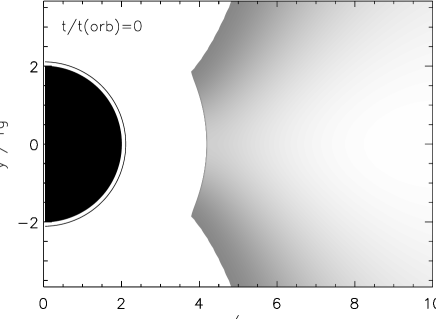
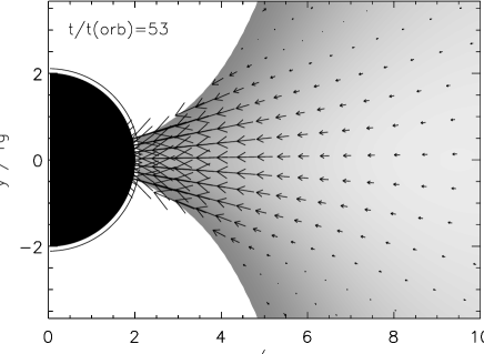
Figure 4: Morphology of the inner part of the disc with parameters $l=3.9136$ and $\Delta W_{\mathrm{in}}=0.16$. Top: initial state; Bottom: final state at $t\simeq 53t_{\mathrm{orb}}$. The arrows are proportional to the components $\left(S_{r}/\sqrt{g_{rr}},S_{\theta}/\sqrt{g_{\theta\theta}}\right)$ of the momentum and are plotted only in the region where $\rho\geq 0.05\ \rho^{0}_{\mathrm{max}}$. The black hole is represented by the black circle and the exterior circle around it marks the location of the inner boundary of the grid.

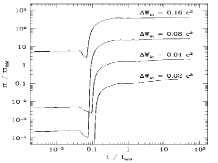
Figure 5: Time evolution of the mass flux for a stationary model with $l=3.9136$ and $\Delta W=0.02$, $0.04$, $0.08$ and $0.16$. The time is given in units of the orbital period at the center (see text), which here is $t_{\mathrm{orb}}\simeq 187\ r_{\mathrm{g}}/c$. The mass flux is normalized with the Eddington limit computed with $M_{\mathrm{BH}}=1\ \mathrm{M}_{\odot}$. For a different choice of polytropic constant $\kappa$ and black hole mass $M_{\mathrm{BH}}$, the mass flux scales as $\kappa^{-3}M_{\mathrm{BH}}$ for $\gamma=4/3$. The initial value of the mass flux is fixed by the spherical mass accretion rate associated with the Bondi flow imposed in the low density regions outside the torus. Notice that after a transition phase lasting for $\sim 0.1\ t_{\mathrm{orb}}$ the mass accretion rate rapidly tends, asymptotically, to the stationary values.

As a representative example Figure 4 shows the morphology of the model with $\Delta W_{\mathrm{in}}=0.16$. The cusp is located at $r_{\mathrm{cusp}}=4.197$ and the center at $r_{\mathrm{center}}=9.598$. The grid extends to $r_{\mathrm{max}}=35$. The top panel shows a gray-scale plot of the logarithm of the density for the initial model at $t=0$, together with the corresponding velocity field. The bottom panel shows the same morphology at the final time $t=10^{4}$. This corresponds to about 53 dynamical timescales, choosing as a dynamical timescale the orbital period $t_{\mathrm{orb}}=2\pi/\Omega$ at $r=r_{\mathrm{center}}$, which for this model is $t_{\mathrm{orb}}=184.9$. The code was stopped after roughly $2\times 10^{5}$ iterations with no signs of numerical instabilities present. One can clearly see in Figure 4 that an accretion flow from the disc to the black hole appears in the inner region of the grid. This flow, however, becomes rapidly stationary (see below). In addition, for our particular choice of model parameters, the corresponding mass flux is very low. Therefore, except in the innermost region where the accretion flow develops, the morphology of the disc remains essentially unchanged during the whole evolution from $t=0$ to $t=53t_{\mathrm{orb}}$.

There are some additional noteworthy issues concerning this figure: first, it clearly shows the ability of the code to keep the equatorial plane symmetry of the torus, even though the angular domain extends from $0$ to $\pi$. Second, the smoothness of the initial disc distribution in the grid is maintained during the whole evolution even close to the black hole horizon. Finally, contrary to previous work (Hawley et al. 1984b; Igumenshchev & Beloborodov 1997) there are no hints of vortices developing in the flow. In Hawley et al. (1984b) such vortices are associated to small poloidal velocities and are not as noticeable as in the results of Igumenshchev & Beloborodov (1997). The latter claim, however, that such vortex motions are likely to be related to the choice of initial conditions, developing from initial perturbations close to the cusp and propagating outwards undamped.

A more quantitative proof of the ability of the code in keeping the stationarity of this solution is provided in Figure 5. This figure shows the evolution of the mass accretion rate (normalized to the Eddington value), $\dot{m}/\dot{m}_{\mathrm{Edd}}$, as a function of $t/t_{\mathrm{orb}}$. The mass flux is computed at the innermost radial point as

$$\dot{m}=2\pi\int_{0}^{\pi}\sqrt{-g}Dv^{r}d\theta,$$ (68)

where the volume element for the Schwarzschild metric is given by $\sqrt{-g}=r^{2}\sin\theta$. The Eddington mass flux $\dot{m}_{\mathrm{Edd}}=\frac{L_{\mathrm{Edd}}}{c^{2}}\simeq 1.4\ 10^{17}\ \frac{M_{\mathrm{BH}}}{\mathrm{M}_{\odot}}\ \mathrm{g/s}$ is computed for $M_{\mathrm{BH}}=1\ \mathrm{M}_{\odot}$. Rescaling of $\dot{m}$ for different polytropic constant $\kappa$ and black hole mass $M_{\mathrm{BH}}$ is given by

$$\frac{\left(\dot{m}/\dot{m}_{\mathrm{Edd}}\right)_{1}}{\left(\dot{m}/\dot{m}_{\mathrm{Edd}}\right)_{2}}=\left(\frac{\kappa_{1}}{\kappa_{2}}\right)^{-3}\frac{M_{\mathrm{BH}\ 1}}{M_{\mathrm{BH}\ 2}}\ ,$$ (69)

where $\gamma=4/3$ was assumed. After a transient initial phase the mass accretion rate is seen to rapidly tend, asymptotically, to a constant value. The offset observed during the initial phase corresponds to the spherical accretion mass flux associated with the particular background solution we use outside the torus.

Figure 6: Mass flux $\dot{m}$ as a function of the energy gap $\Delta W_{\mathrm{in}}$ between the inner edge of the disc and the cusp. The dots indicate the asymptotic values we get in our simulations (see Fig. 5). The dashed line shows the slope which is expected from the theoretical prediction given by Eq. (32), which for $\gamma=4/3$ is 4. The plot corresponds to simulations with $M_{\mathrm{BH}}=1\ \mathrm{M}_{\odot}$ and $\kappa=1.5\times 10^{20}\ \mathrm{cgs}$.

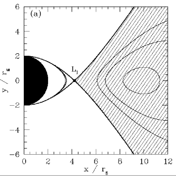
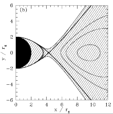
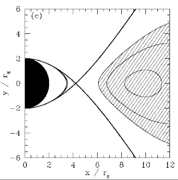
Figure 7: The physical origin of the runaway instability: the initial disc fills its Roche lobe (panel (a)). Mass transfer from the disc to the black hole occurs through the cusp, which is located at the Lagrange point $L_{1}$. The mass of the black hole increases and the disc has to find a new equilibrium configuration with the new gravitational potential. There exist two possibilities: (i) the disc overflows its Roche lobe (panel (b)). This process speeds up the mass transfer and the disc becomes unstable. (ii) The disc contracts inside its Roche lobe (panel (c)), which forces the mass transfer to slow down, resulting on a stable disc.

Next, in Figure 6 we plot the mass flux as a function of the energy gap $\Delta W_{\mathrm{in}}$ for the four stationary models we have considered. The values selected for the mass flux in each model are the asymptotic ones, obtained after the simulations have been evolved up to a final time $t=10^{4}$, roughly 54 orbital periods. This plot allows us to check if the code is able to reproduce the analytic dependence given by Eq. (32). For a $\gamma=4/3$ polytrope the expected slope is 4 (dashed line). As the figure shows our results are in good agreement with this analytic prediction as well as with the numerical results obtained by Igumenshchev & Beloborodov (1997) for the same models.

6 Simulations of the runaway instability

6.1 The physical origin of the instability

Figure 8: The physical origin of the runaway instability: the evolution of models with different mass is plotted against the mass transfered from the disc to the black hole. The initial disc is filling its Roche lobe (indicated by the big dot symbol). Initially $M_{BH}=2.44\ \mathrm{M}_{\odot}$ and $M_{D}=0.36\ \mathrm{M}_{\odot}$. Upper panel: mass $M_{\mathrm{BH}}$ of the black hole; Lower panel : mass $M_{\mathrm{D}}$ of the disc and mass $\mathrm{M}_{\mathrm{D}}^{\mathrm{max}}$ contained inside the Roche lobe (dashed line). As $M_{\mathrm{D}}\geq M_{\mathrm{D}}^{\mathrm{max}}$, the disc overflows its Roche lobe which speeds up the mass transfer and leads to the runaway instability.

The physical mechanism leading to the runaway instability has been explained by Abramowicz et al. (1983) and Nishida et al. (1996). The mass transfer from the disc to the black hole starts once the disc fills its Roche lobe (see Fig. 7a). From this moment any small perturbation allows the gas to flow through the cusp located at the inner edge of the disc. As a result the mass of the black hole increases, the equipotential surfaces move, and the radial location of the cusp changes. The disc has to find a new equilibrium configuration: one possibility is that the disc overflows its Roche lobe as is depicted in Fig. 7b. In this case the mass transfer speeds up, which leads to the runaway instability. Alternatively, the disc may contract inside its Roche lobe (see Fig. 7c). In this case the mass transfer slows down. The mass flux is self-regulated by this process and the accretion is stable.

However, for a Schwarzschild black hole and a constant angular momentum distribution in the disc, most discs are unstable (Abramowicz et al. 1983) (see also Table 1). This is illustrated in Fig. 8 for the particular case where the black hole mass is $M_{\mathrm{BH}}=2.44\ \mathrm{M}_{\odot}$, the disc mass is $M_{\mathrm{D}}=0.36\ \mathrm{M}_{\odot}$, the adiabatic index is $\gamma=4/3$ and the polytropic constant is $\kappa=4.76\times 10^{14}\ \mathrm{cgs}$ (which corresponds to degenerate relativistic electrons with $Y_{\mathrm{e}}=0.5$ electrons per nucleon). In this figure the evolution of models with different mass is plotted against the mass transfered from the disc to the black hole. The initial disc is filling its Roche lobe. The location of both the initial disc mass and black hole mass is indicated by a big dot symbol in each panel. The upper panel shows the evolution of the mass of the black hole whereas the lower one shows the corresponding evolution of the disc and of $\mathrm{M}_{\mathrm{D}}^{\mathrm{max}}$, which is the maximum disc mass contained inside the Roche lobe (dashed line). As $M_{\mathrm{D}}\geq M_{\mathrm{D}}^{\mathrm{max}}$, the disc overflows its Roche lobe which speeds up the mass transfer and leads to the runaway instability.

6.2 The sequence of stationary metrics approximation

The increase of the mass of the black hole is the fundamental process triggering the runaway instability. In order to properly take into account the dynamical evolution of the underlying gravitational field, one should solve the coupled system of Einstein and hydrodynamic equations. However, such a task has not yet been accomplished in the context of the runaway instability and, to some extent, it may be still far from the capabilities of current codes in numerical relativity. Numerical stability considerations, coming from both the coordinate singularity existing at the rotation axis ($\theta=0,\pi$), which spoils the long-term integration of the Einstein equations even in vacuum (Brandt & Seidel 1995), and from the mathematical formulation of the field equations themselves, make such a task very challenging. Numerical relativity codes evolving black hole spacetimes with perfect fluid matter are only becoming available very recently, both in axisymmetry (Brandt et al. 2000) as in full 3D (Shibata & Uryū 2000; Shibata et al. 2000; Alcubierre et al. 2000; Font et al. 2001). Nevertheless, the resolution and the integration times required to study the time evolution of the runaway instability may be still too demanding for such relativistic codes which incorporate self-gravity.

For all these reasons and for the complete lack of time-dependent simulations of the runaway instability in relativity, we have adopted a simplified and pragmatic approach to the problem. In our procedure the spacetime metric is approximated at each time step by a stationary exact black hole metric of varying mass (and angular momentum in the case of a rotating black hole). The mass $M$ of the black hole necessary to compute the metric coefficients is increased at each time step $\Delta t$ according to:

$$M^{n+1}=M^{n}+\Delta t\ \dot{m}^{n}\ ,$$ (70)

where the mass flux at the inner radius of the grid is evaluated by the equation

$$\dot{m}^{n}=2\pi r_{i_{\mathrm{min}}}^{2}\Sigma_{j=1}^{j_{\mathrm{max}}}\left(\theta_{j+1}-\theta_{j}\right)\sin\theta_{j}D_{i_{\mathrm{min}}j}v^{r}_{i_{\mathrm{min}}j}.$$ (71)

As the mass of the black hole increases during the simulations, the horizon moves outwards. To avoid the inner radius of the grid to become smaller than the radius of the growing horizon, we increase the index $i_{\mathrm{min}}$ of the first radial zone when necessary, so that the condition $r_{i_{\mathrm{min}}}>2M$ is always respected. We notice that the black hole mass increases very slowly during the evolution which implies that the metric coefficients at any time step differ very little from the final values which would correspond to an exact Schwarzschild black hole of bigger mass but with no matter around.

6.3 Initial state

A given initial state of the black hole plus disc system is determined by five parameters: the mass of the black hole $M_{\mathrm{BH}}$, the specific angular momentum in the disc $l$, the potential at the inner edge of the disc $\Delta W_{\mathrm{in}}$, the polytropic constant $\kappa$ and the adiabatic index $\gamma$. The computing time needed for one hydrodynamical simulation is too large to allow for a complete exploration of this parameter space. For this reason we focus on those models which are expected to be found in the central engine of GRBs. These systems are formed either after the coalescence of two compact objects or after the gravitational collapse of a massive star.

Table 3: Initial models. The following parameters are listed: mass of the black hole $M_{\mathrm{BH}}$, disc-to-hole mass ratio $M_{\mathrm{D}}/M_{\mathrm{BH}}$, specific angular momentum in the disc $l$, potential barrier at the inner edge $\Delta W_{\mathrm{in}}$, mass flux in the stationary regime $\dot{m}_{\mathrm{stat}}$, minimum and maximum radii of the grid, $r_{\mathrm{min}}$ and $r_{\mathrm{max}}$, radius of the cusp $r_{\mathrm{cusp}}$, radius of the center $r_{\mathrm{center}}$ (all radii are in units of the gravitational radius $r_{\mathrm{g}}$), and orbital period at the center of the disc $t_{\mathrm{orb}}$. The last column lists the timescale associated with the runaway instability as defined in Section 6.4. In all cases, the EoS parameters are $\kappa=4.76\times 10^{14}\ \mathrm{cgs}$ and $\gamma=4/3$.

Model	$M_{\mathrm{BH}}$	$M_{\mathrm{D}}/M_{\mathrm{BH}}$	$l$	$\Delta W_{\mathrm{in}}$	$\dot{m}_{\mathrm{stat}}$	$r_{\mathrm{min}}$	$r_{\mathrm{max}}$	$r_{\mathrm{cusp}}$	$r_{\mathrm{center}}$	$t_{\mathrm{orb}}$	$t_{\mathrm{run}}/t_{\mathrm{orb}}$
	$(\mathrm{M}_{\odot})$				$(\mathrm{M_{\odot}/s})$				(geo/ms)
1a	2.5	1.	3.9325	0.005	0.090	2.1	85.∗	4.1492	9.7930	193. / 2.37	97. / $95.^{\dagger}$
2a	2.5	1.	3.9085	0.01	0.28	2.1	85.∗	4.2105	9.5455	185. / 2.28	38. / 36.†
3a	2.5	1.	3.8564	0.02	2.1	2.1	85.∗	4.3639	8.9919	169. / 2.09	10. / 9.2†
4a	2.5	1.	3.7255	0.04	34.	2.1	85.∗	5.0104	7.3644	126. / 1.55	3.8 / 3.3†
1b	2.5	0.1	3.8749	0.005	0.032	2.1	37.	4.3058	9.1915	175. / 2.16	140.
2b	2.5	0.1	3.8459	0.01	0.17	2.1	37.	4.3990	8.8768	166. / 2.05	64.
3b	2.5	0.1	3.7798	0.02	1.9	2.1	37.	4.6698	8.1077	145. / 1.79	12.
1c	2.5	0.05	3.8798	0.001	0.21	2.1	32.	4.2911	9.2438	177. / 2.17	110.

∗ In models 1a to 4a the grid consists of a first grid from $r=2.1$ to $r=28$ and a second grid from $r=28$ to $r=85$ to avoid $\Delta r$ at

the inner radius becoming too large.

† The second estimate of $t_{\mathrm{run}}$ given for models 1a to 4a corresponds to simulations where the mass of the black hole starts to increase

only once the stationary regime has been reached (see Section 6.4).

6.3.1 Black hole mass and disc-to-hole mass ratio

As it has been shown by numerical simulations using Newtonian and post-Newtonian gravity, both the coalescence of two neutron stars (Ruffert & Janka 1999) and the merger of a black hole and a neutron star (Kluzniak & Lee 1998) lead to the formation of comparable systems, where the mass of the central black hole and the disc-to-hole mass ratio are respectively $M_{\mathrm{BH}}\sim 2.5\ \mathrm{M_{\odot}}$ and $M_{\mathrm{D}}/M_{\mathrm{BH}}\sim 0.04$–$0.08$ for the first case, and $M_{\mathrm{BH}}\sim 3\ \mathrm{M_{\odot}}$ and $M_{\mathrm{D}}/M_{\mathrm{BH}}\sim 0.2$ in the second case. More recently, the fully relativistic simulations of binary neutron star coalescence performed by Shibata & Uryū (2000) yield disc masses of $\sim 0.05-0.1M_{*}$ for corotational binaries and $<0.01M_{*}$ for irrotational binaries, where $M_{*}$ is the total rest-mass of the system (typically $\sim 2M_{\odot}$).

The case of collapsars is more complex since, in particular, the mass of the disc goes on increasing after the formation of the black hole, as matter from the outer parts of the star is still infalling. The simulations performed by MacFadyen & Woosley (1999) and Aloy et al. (2000) start from the $14\ \mathrm{M_{\odot}}$ helium core of a rotating $35\ \mathrm{M_{\odot}}$ main sequence star which collapses to produce a central black hole surrounded by a disc. When this systems enters a quasi-steady state, the mass of the black hole is $2$–$3\ \mathrm{M_{\odot}}$ and the disc-to-hole mass ratio is typically about $0.001$–$0.01$.

Taking into account these various results, we have decided to fix the mass of the black hole to $M_{\mathrm{BH}}=2.5\ \mathrm{M_{\odot}}$ and to adjust the angular momentum $l$ to get realistic disc-to-hole mass ratios. We have considered three possible ratios: $0.05$, $0.1$ and $1$. Such values are very close to what is obtained in the simulations of binary coalescence and not too far from the results of the simulations of collapsars.

6.3.2 Equation of state

We fix the adiabatic index to $\gamma=4/3$ and the polytropic constant to $\kappa=1.2\times 10^{15}\ Y_{\mathrm{e}}^{4/3}$ with $Y_{\mathrm{e}}=0.5$. This corresponds to an EoS dominated by the contribution of relativistic degenerate electrons (the typical density in the disc is $\sim 10^{11}$-$10^{12}\ \mathrm{g/cm^{3}}$). We note that such simplified EoS is nevertheless adequate to our purpose since the work of Nishida & Eriguchi (1996) showed that, for stationary models, the effects of realistic EoS on the stability of constant angular momentum discs is negligible, the discs being unstable in all cases.

6.3.3 Mass flux

Once $M_{\mathrm{BH}}$, $M_{\mathrm{D}}/M_{\mathrm{BH}}$, $\kappa$ and $\gamma$ have been specified, the only remaining parameter is the potential at the inner edge of the disc, $\Delta W_{\mathrm{in}}$. We choose its value so that the corresponding mass flux in the stationary regime (as described in Section 5) explores a realistic range. In the simulations of binary neutron star coalescence carried out by Ruffert & Janka (1999), the mass accretion rate of the black hole varies between $1$ and $10^{4}\ \mathrm{M_{\odot}/s}$. On the other hand, Kluzniak & Lee (1998) find comparable values in the case of a neutron star - black hole merger. In their simulations of collapsars, MacFadyen & Woosley (1999) find a typical mass flux of $0.6$–$0.8\ \mathrm{M_{\mathrm{\odot}}/s}$.

Such mass fluxes are many orders of magnitude larger than the Eddington limit, which is $1.2\times 10^{-16}\ \mathrm{M_{\odot}/s}$ for a $M_{\mathrm{BH}}=2.5\ \mathrm{M}_{\odot}$. However such very high mass fluxes are precisely what is required to explain the observed luminosity of GRBs, which is typically $L_{\mathrm{\gamma}}=10^{51}\ L_{51}\ \mathrm{erg/s}$ in gamma-rays. If this radiation is due to internal shocks propagating within an ultra-relativistic wind, the kinetic energy flux of this wind is $L_{\mathrm{kin}}=L_{\mathrm{\gamma}}/f_{\mathrm{\gamma}}$, where $f_{\mathrm{\gamma}}$ is the efficiency of the kinetic energy to radiation conversion. If one assumes that the production of the relativistic wind is accretion-powered with an efficiency $f_{\mathrm{acc}}$, then the mass flux is given by

$$\dot{m}=\frac{1}{f_{\mathrm{acc}}}\frac{L_{\mathrm{kin}}}{c^{2}}=0.2\ \left(\frac{f_{\mathrm{acc}}}{0.05}\right)^{-1}\left(\frac{f_{\mathrm{\gamma}}}{0.05}\right)^{-1}L_{51}\ \mathrm{M_{\odot}/s}\ .$$ (72)

This estimate is of course no longer relevant if the main energy reservoir powering the burst is the rotational energy of the black hole, which can be extracted by the Blandford-Znajek effect (Blandford & Znajek 1977).

Taking into such high mass fluxes we have considered the following values of $\Delta W_{\mathrm{in}}$: 0.001, 0.005, 0.01, 0.02 and 0.04 so that the mass flux of our initial models in the stationary regime spans $\sim 0.03$–$30\ \mathrm{M_{\odot}}/s$. From all the above considerations we have prepared eight initial models which are summarized in Table 3.

6.4 Results

Each of our eight initial models is evolved twice: in the first series of runs we keep constant the mass of the black hole while in the second set of evolutions such mass is allowed to increase according to the law specified in the preceding section, Eqs. (70) and (71). For the first type of runs the mass flux rapidly reaches a stationary regime (like in the models discussed in Section 5) which can be maintained for as long as desired. In practice the final time corresponds to many orbital periods of the disc. The mass flux at this stage has the value reported as $\dot{m}_{\mathrm{stat}}$ in Table 3. On the other hand, when the mass of the black hole increases (second series of runs), the time evolution of the system changes dramatically and the runaway instability appears.

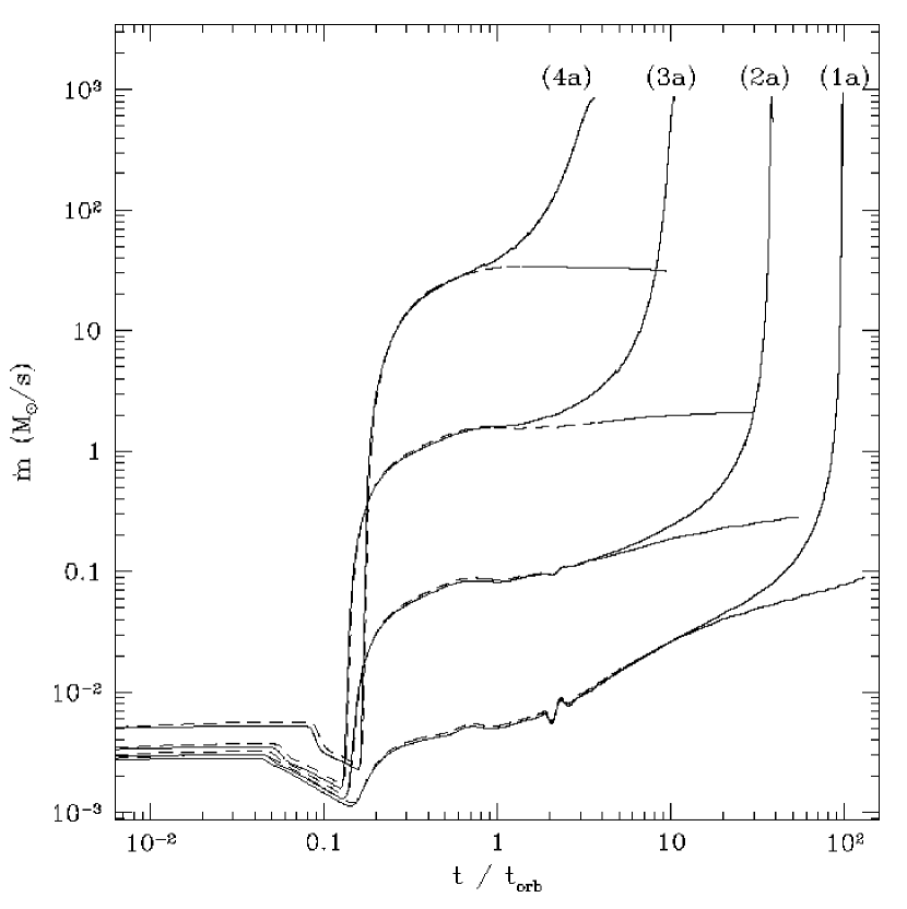
Figure 9: Time-evolution of the mass flux for models (1a) to (4a) of Table 3. The solid lines correspond to evolutions in which the black hole mass increases with time according to the procedure explained in Section 6.2. For comparison, the mass flux in the stationary regime (when the mass of the black hole is kept constant) is also plotted using dashed lines. As expected, for a black hole of growing mass the accretion process becomes rapidly unstable. Notice how the mass flux diverges.

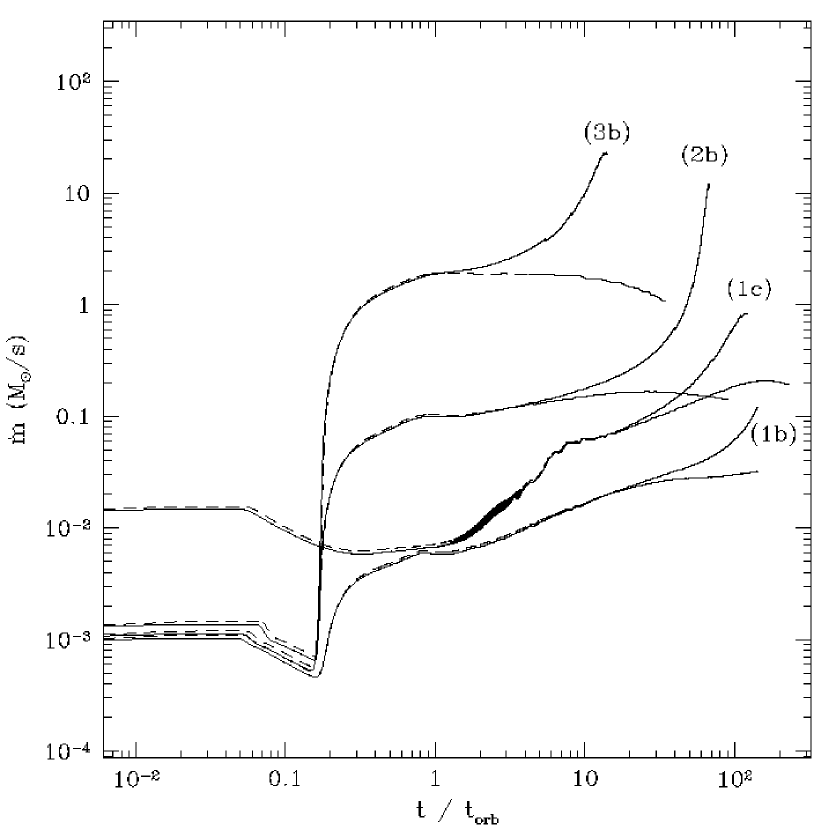
Figure 10: Time-evolution of the mass flux for models (1b) to (3b) and model (1c) of Table 3. As in Fig. 9, the solid lines correspond to evolutions in which the black hole mass increases with time according to the procedure explained in Section 6.2 and the dashed lines correspond to evolutions in which the mass of the black hole is kept constant. As expected, for a black hole of growing mass the accretion process becomes rapidly unstable. Notice how the mass flux diverges.

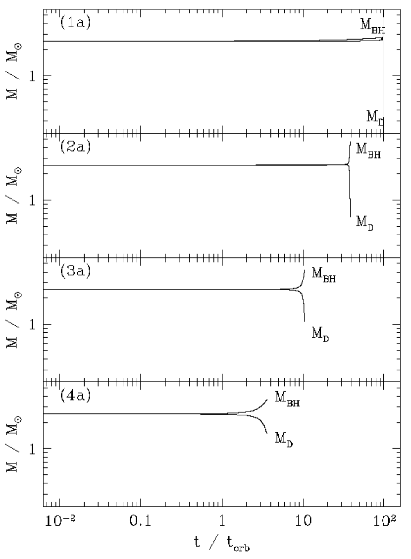
Figure 11: Time-evolution of the mass of the black hole and of the mass of the disc for models (1a) to (4a) listed in Table 3. The sudden appearance of the instability is noticeable. The increase of the black hole mass is directly associated with the corresponding decrease in the mass of the disc.

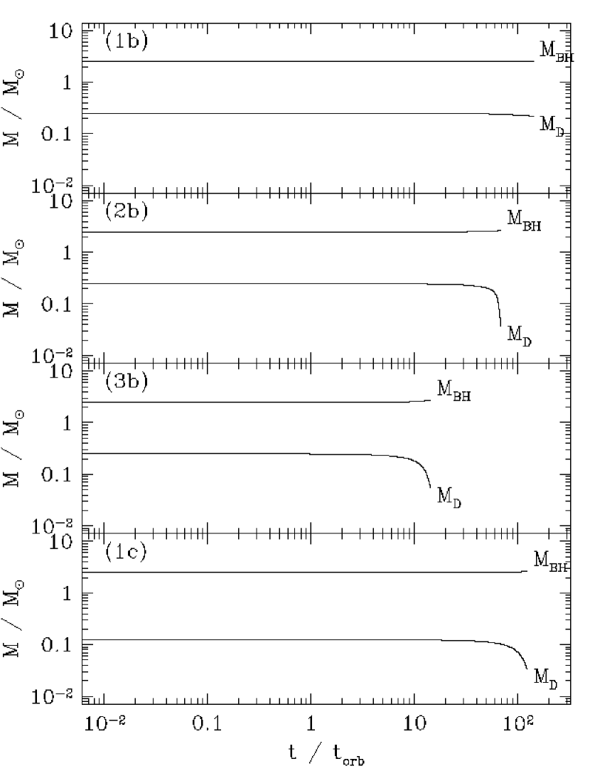
Figure 12: Time-evolution of the mass of the black hole and of the mass of the disc for models (1b) to (3b) and model (1c) of Table 3. Since the mass of the disc is now much smaller than in models labeled ‘a’ the growth of the black hole mass is not as clearly visible as in Fig. 11. The sudden decrease of the mass of the disc is however noticeable.

The dramatic differences between both series of simulations are depicted in Figures 9-12. Figures 9 and 10 show the time evolution of the mass accretion rate for models (1a) to (4a) and (1b) to (3b) plus (1c), respectively. They include, both, the stationary and the unstable cases. The overall behaviour found in both figures is similar despite the existing different mass ratio between the black hole and the disc, 1 in all curves of Fig. 8 and 0.1 and 0.05 in those of Fig. 9. The different mass ratio only affects the mass flux and (weakly) the time in which the instability appears. So, in models labeled ‘b’ and ‘c’ the instability takes somewhat more time to appear than in the corresponding models ‘a’ with the same energy gap (see below). As a result, models labeled ‘b’ and ‘c’ need more computational time to be fully evolved. This fact sets important technical restrictions when trying to evolve models with smaller mass ratio for which neglecting the disc self-gravity would be more justified. Short-term evolutions of a model with a 0.01 disc-to-hole mass ratio show that the instability is indeed present but simply takes longer to grow.

In Figures 9 and 10 we see that at early times the evolution of the mass flux for each pair of models is exactly the same, irrespective of the increase of the black hole mass being taken into account or not. However, whereas the models with a constant black hole mass reach a quasi-stationary regime with a constant mass flux, the corresponding mass accretion rate for those models with an increasing black hole mass goes on increasing after having reached the ‘stationary’ value. Furthermore, the time derivative of the mass flux also increases, which implies that the mass flux diverges rapidly. For all unstable models computed the mass flux is already several orders of magnitude larger than the stationary value when the calculation is stopped. (4 orders of magnitude for Model (1a)!, see Fig. 9). The divergence found in the mass accretion rate is a clear manifestation of the runaway instability at work, which leads ultimately to the complete destruction of the disc.

In Figs. 11 and 12 we plot the time-evolution of the black hole mass and the disc mass for the same set of models displayed in Figs. 9 and 10, respectively. The sudden loss of the mass of the disc at late times is reflected on the corresponding rapid increase of the mass of the black hole. As an example, for Model (2a), at $t\sim 40\ t_{\rm orb}$ the black hole has almost doubled its mass ($M_{\rm BH}\sim 4.7\ \mathrm{M}_{\odot}$) and, correspondingly, the mass of the disc has decreased from $2.5\ \mathrm{M}_{\odot}$ to roughly $0.3\ \mathrm{M}_{\odot}$. Note that since models ‘b’ and ‘c’ have a much smaller disc mass than models ‘a’ the growth of the black hole mass in Fig. 12 is not as clearly visible as in Fig. 11.

The morphology changes that the unstable system undergoes are shown in Figure 13 for a representative case (Model 3a). The evolution is qualitatively similar for all models. In this figure we show eight snapshots of the time-evolution from $t=0$ to $t=11.8\ t_{\rm orb}$. The variable plotted in the figure is the rest-mass density. The contour levels are linearly spaced with $\Delta\rho=0.1\ \rho_{\mathrm{c}}^{0}$, where $\rho_{\mathrm{c}}^{0}$ is the maximum value of the density at the center of the initial disc. In Fig. 13 one can clearly follow the transition from a quasi-stationary accretion regime (panels (1) to (5)) to the rapid development of the runaway instability (panels (6) to (8)). At $t=11.80\ t_{\mathrm{orb}}$, the disc has almost entirely disappeared inside the black hole whose size has noticeably grown. From the numerical point of view, and as already pointed out in Section 5 when describing stationary models, the flow solution remains considerably smooth even though the evolution is now dynamic. The equatorial plane symmetry is maintained during the whole evolution with no sign of numerical asymmetries as well as no vortices appearing inside the disc.

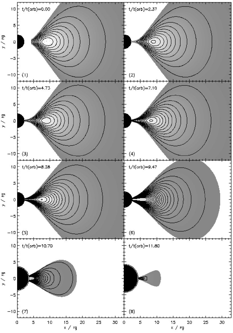
Figure 13: Time evolution of the unstable model (3a): contour levels of the rest-mass density $\rho$ plotted at irregular times from $t=0$ to $t=11.80\ t_{\mathrm{orb}}$ once the disc has almost been entirely destroyed. The density levels are linearly spaced with $\Delta\rho=0.1\ \rho_{\mathrm{c}}^{0}$. The density $\rho_{\mathrm{c}}^{0}$ takes the value at the center of the initial disc (marked by a dot in panel (1)). The most exterior contour corresponds to $\rho=0.1\ \rho_{\mathrm{max}}^{0}$. The entire disc is filled in grey color. From panels (1) to (3) the disc is very close to a stationary regime and it is almost not evolving. The runaway instability develops from panels (4) to (8), most noticeable in the last three panels from time $t=9.47\ t_{\mathrm{orb}}$ to $t=11.80\ t_{\mathrm{orb}}$. The increase in the central density and the infall of the disc to the black hole are well visible, as well as the associated growth of the black hole.

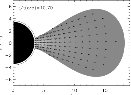
Figure 14: Unstable Model (3a): velocity field at $t=10.70\ t_{\mathrm{orb}}$ (corresponding to snapshot (7) in Fig. 13). The arrows are proportional to $v^{i}$ and are plotted only in the region where $\rho\geq 0.1\ \rho^{0}_{\mathrm{max}}$.

Figure 15: Time-evolution of the mass flux for model (4a) of Table 3. As in Figure 9, the dashed line corresponds to the case where the mass of the black hole is kept constant whereas the thin solid line corresponds to the case where the mass of the black hole increases (from $t=0$). In addition, the thick solid line corresponds to a third case in which the mass of the black hole starts to increase only at time $t_{0}=7.9\ t_{\mathrm{orb}}$ (indicated by a vertical arrow), i.e. once the mass flux has reached its ‘stationary value’. In this case the instability shows up immediately. However, the timescale is the same than in the previous run (thin solid line; notice the logarithmic scale for $t$).

Correspondingly, Figure 14 shows the velocity field for model (3a) at $t=10.70t_{\rm orb}$, associated with snapshot (7) in Fig. 13). This figure shows that the disc is falling radially on to the black hole with no signs of vortices and circulation patterns developing.

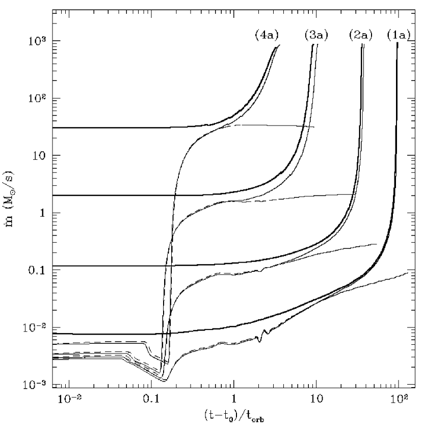
Figure 16: Time-evolution of the mass flux as a function of $t-t_{0}$ for models (1a) to (4a) of Table 3, where $t_{0}$ is the time at which the mass of the black hole starts to increase. As in Figure 9, the dashed lines correspond to the case where the mass of the black hole is kept constant whereas the thin solid lines correspond to the case where the mass of the black hole increases ($t_{0}=0$). The thick solid lines show the evolution when the mass of the black hole starts to increase only from time $t_{0}$, equal to 1000, 200, 24 and 7.9 $t_{\mathrm{orb}}$ for models (1a) to (4a) respectively, i.e. once the mass flux has reached its ‘stationary value’. In such case, the runaway instability appears earlier, the effect being more important for models (1a) and (2a).

Figure 17: The timescale of the runaway instability $t_{\mathrm{run}}$ (as defined in Section 6.4) is plotted as a function of the mass flux $\dot{m}_{\mathrm{stat}}$ in the ‘stationary regime’ for each of the models listed in Table 3. For models (1a) to (4a) ($M_{\mathrm{D}}/M_{\mathrm{BH}}=1.$), we use the more accurate estimate of $t_{\mathrm{run}}$ obtained when the mass of the black hole starts to increase once the stationary regime has been reached. The dashed line corresponds to the best fit $t_{\mathrm{run}}\propto\dot{m}_{\mathrm{stat}}^{-\alpha}$ for this series. We find $\alpha=0.9$.

An interesting information which our hydrodynamical simulations provide is the timescale of the instability $t_{\mathrm{run}}$. We estimate this timescale as the time it takes for half of the mass of the disc to fall into the hole. The values of $t_{\mathrm{run}}$ obtained for our 8 models are given in the last column of Table 3. Such values span the interval $\sim 3.8$–$140t_{\mathrm{orb}}$, which corresponds to very small durations ($\sim 6$–$300\ \mathrm{ms}$). To check the quality of our definition of $t_{\mathrm{run}}$ we have performed the following test: for the four models of series ‘a’ we have carried out additional simulations in which the mass of the black hole starts to increase only once the stationary regime has been reached at time $t\simeq t_{0}$. The corresponding evolution of the mass flux in case (4a), for which $t_{0}\simeq 7.9\ t_{\mathrm{orb}}$, is plotted in Fig. 15. To compare more easily the timescale associated with the runaway instability in the two cases, we have plotted in Fig. 16 the evolution of the mass flux as a function of $t-t_{0}$. Again we see that in all cases the runaway instability appears immediately resulting in the rapid disappearance of the disc. However the precise comparison between our usual series of runs (where $t_{0}=0$) and the modified ones leads to the conclusion that the timescale of the runaway instability is a bit overestimated in the first case. The new values of the timescale for series ‘a’ are reported in the last column of Table 3.

In Fig. 17 we plot the timescale $t_{\mathrm{run}}$ as a function of the mass flux in the stationary regime $\dot{m}_{\mathrm{stat}}$. To be able to derive an empirical law for the timescale of the instability one should consider a much larger sample of models. Nevertheless, two clear tendencies can already be extracted from this figure: (i) the timescale depends weakly on the disc-to-hole mass ratio; (ii) the runaway instability occurs faster when the initial mass flux (stationary value) is larger, following approximatively $t_{\mathrm{run}}\propto\dot{m}^{-\alpha}$. With the value of $\alpha=0.9$ obtained for series ‘a’ (where we have used the result of the modified runs to get a more accurate estimate of $t_{\mathrm{run}}$), we can infer that, for all cases, the disc is destroyed in a duration never exceeding $1\ \mathrm{s}$ for a large range of accretion mass fluxes, $\dot{m}_{\mathrm{stat}}\ga 10^{-3}\ \mathrm{M_{\odot}/s}$.

7 Conclusions

We have presented results from a numerical study of the runaway instability of thick discs around black holes. In this study we have carried out a comprehensive set of time-dependent simulations aimed at exploring the appearance of the instability. In order to do so we have used a fully relativistic, axisymmetric hydrodynamics code. The general relativistic hydrodynamic equations have been formulated as a first-order, flux-conservative hyperbolic system and solved using a suitable Godunov-type scheme. Among the simplifying conditions we have assumed a constant angular momentum disc around a Schwarzschild (nonrotating) black hole. The self-gravity of the disc has been neglected and the evolution of the central black hole has been assumed to be that of a sequence of exact Schwarzschild black holes of varying mass.

We have found that by allowing the mass of the black hole to grow the runaway instability appears on a dynamical timescale. The mass flux diverges and the disc entirely falls into the hole in a few orbital periods (1 $\to$ 100). Therefore, the appearance of the runaway instability in constant angular momentum discs found in our simulations is in complete agreement with previous estimates from stationary models (Abramowicz et al. 1983; Nishida et al. 1996). Our simulations provide the first estimation of the timescale associated with the runaway instability. For a black hole of $2.5\ \mathrm{M_{\odot}}$ and disc-to-hole mass ratios between 1 and 0.05 this timescale never exceeds $1\ \mathrm{s}$ for a large range of mass fluxes and it is typically about $50\ \mathrm{ms}$. We have found that the dependence of the timescale on the disc-to-hole mass ratio is weak and that the runaway instability occurs faster the larger it is the initial mass flux (stationary regime) from the disc to the black hole.

We note that our study has been restricted to a polytropic gas, with a particular choice of $\kappa$ and $\gamma$ corresponding to a gas of degenerate relativistic electrons. We are aware of the over-simplification of such an EoS. However, the work of Nishida & Eriguchi (1996) has shown that the conclusion of Nishida et al. (1996) (where stationary models were built in a fully relativistic computation including the self-gravity of the disc) is not modified when using a realistic EoS: constant angular momentum discs are unstable. Therefore, we believe that our results would not be strongly modified if we were using a more elaborate description of the matter.

To close our investigation we notice that there are four important limitations in our study: (i) it is difficult to check the validity of our simple-minded approach to incorporate the effect of the black hole mass increase; (ii) the self-gravity of the disc has not been included. Studies based on sequences of equilibrium configurations have shown that it favors the instability (Nishida et al. 1996; Masuda et al. 1998); (iii) the rotation of the black hole and the possible increase of its spin due to the transfer of angular momentum (associated with the transfer of mass) is not yet included in our current model; (iv) the case of a more realistic distribution of angular momentum in the disc (i.e. increasing outwards) has also not been considered yet.

The first two points in the above list cannot be improved without solving the coupled system of Einstein and hydrodynamic equations on black hole spacetimes. Although important advances in the field of numerical relativity this task is still challenging. The other items, however, can be more easily improved and work in this direction will be presented in subsequent investigations. In particular, we will present in a forthcoming paper the effect of a non-constant angular momentum in the disc. Such a distribution of angular momentum is believed to suppress the runaway instability according to previous studies in a stationary framework (e.g. Daigne & Mochkovitch (1997)). This last point - and the very existence of the runaway instability itself - is very important in the context of the most discussed scenario for GRBs. In the standard model the central engine responsible for the highly energetic emission is a thick disc orbiting a stellar mass black hole, with a high accretion mass flux. The lifetime of this system must necessarily be larger than a few seconds to explain the observed durations of the bursts. Our results show that it would be absolutely excluded if the runaway instability occurs.

References

- Abramowicz (1974) Abramowicz M. A., 1974, Acta Astron., 24, 45
- Abramowicz et al. (1983) Abramowicz M. A., Calvani M., Nobili L., 1983, Nature, 302, 597
- Abramowicz et al. (1998) Abramowicz M. A., Karas V., Lanza A., 1998, A&A, 331, 1143
- Alcubierre et al. (2000) Alcubierre M., Brügmann B., Dramlitsch T., Font J. ., Papadopoulos P., Seidel E., Stergioulas N., Takahashi R., 2000, Phys. Rev. D, 62, 044034
- Aloy et al. (2000) Aloy M. A., Müller E., Ibáñez J. M., Martí J. M., MacFadyen A., 2000, ApJ, 531, L119
- Banyuls et al. (1997) Banyuls F., Font J. A., Ibáñez J. M., Martí J. M., Miralles J. A., 1997, ApJ, 476, 221
- Baring & Harding (1997) Baring M. G., Harding A. K., 1997, ApJ, 491, 663
- Blandford & Znajek (1977) Blandford R. D., Znajek R. L., 1977, MNRAS, 179, 433
- Brandt et al. (2000) Brandt S., Font J. A., Ibáñez J. M., Massó J., Seidel E., 2000, Comput. Phys. Comm., 124, 169
- Brandt & Seidel (1995) Brandt S. R., Seidel E., 1995, Phys. Rev. D, 52, 856