Physical Parameter Eclipse Mapping of the quiescent disc in V2051 Ophiuchi

Abstract

We analyse simultaneous UBVR quiescent light curves of the cataclysmic variable V2051 Oph using the Physical Parameter Eclipse Mapping method in order to map the gas temperature and surface density of the disc for the first time. The disc appears optically thick in the central regions and gradually becomes optically thin towards the disc edge or shows a more and more dominating temperature inversion in the disc chromosphere. The gas temperatures in the disc range from about 13 500 K near the white dwarf to about 6 000 K at the disc edge. The intermediate part of the disc has temperatures of 9 000 K to 6 500 K.

The quiescent disc (chromosphere) shows a prominent bright region with temperatures of 10 500 K around the impact region of the stream from the secondary with an extension towards smaller azimuths. The disc has a size of $0.53\pm 0.03R_{\SS L1}$ and a mass accretion rate of between $\dot{\cal M}=10^{15}$gs^-1to $10^{17}$gs^-1. The light curves must include an uneclipsed component, a hot chromosphere and/or a disc wind.

The PPEM method allows us to determine a new distance of $146\pm 20$ pc, compatible with previous rough estimates. For the white dwarf we then reconstruct a temperature of 19 600 K, if the lower hemisphere of the white dwarf is occulted by the disc.

We suggest that the accretion disc is a sandwich of a cool, optically thick central disc with hot chromospheric layers on both sides as was suggested for HT Cas. This chromosphere is the origin of the emission lines.

We find that although V2051 Oph is very similar to the SU UMa type dwarf novae HT Cas, OY Car and Z Cha, there must be a substantial difference in order to explain its unique light curve. The reason for the difference could either be a higher mass transfer rate caused by the more massive secondary and/or a small but significant magnetic field of the white dwarf, just strong enough to dissrupt the innermost disc.

1 Introduction

The eclipsing cataclysmic variable (CV) V2051 Oph was discovered by Sanduleak (1972). Since then, the classification as a CV was quite certain, but not, of which subtype. Bond & Wagner (1977) suggested it might be of AM Her type and this idea was supported by Warner & O’Donoghue (1987), hereafter WO, refining the classification to a low-field polar. Other studies are based on the assumption that V2051 Oph is a dwarf nova (Watts et al. 1986, Baptista et al. 1998) with infrequent outbursts and low states (Warner & Cropper 1983, Baptista et al. 1998). V2051 Oph shows typical features of a high inclination dwarf nova exhibiting an accretion disc, like double peaked emission lines.

The mystery of V2051 Oph seemed to be solved with the detection of a super outburst during which superhumps were detected (Kiyota & Kato 1998). Since then, the system was classified as an SU UMa type dwarf nova. Therefore, we assume this system to exhibit an accretion disc. This is further supported by Baptista et al. (1998) who do not find typical features of a polar in their light curves of V2051 Oph, like wanderings of ingress and egress phases or large amplitude pulsations. However, in order to explain the complex behaviour of V2051 Oph, Warner (1996) suggests that this system is a polaroid, an intermediate polar with a synchronized primary.

With 1.5^h it has a rather short orbital period, very similar to HT Cas, OY Car and Z Cha and in fact it is often compared to these. However, the accretion disc seems to be highly variable, as apparent from the variable eclipse profiles. Sometimes the disc seems to be only small, hot and sharply defined, while at other times the disc appears to be more extended (Warner & Cropper 1983). Furthermore, at times it shows a hump in the light curve with variable timing (before or after eclipse) and variable occurance (it can occur at one eclipse and disappear at the next) (WO). At other times, no such hump is observed (e.g. this paper).

As V2051 Oph is an eclipsing system, the system parameters are quite well known (e.g. Baptista et al. 1998). However, the lack of traces of the secondary even in the infra-red prevents pinning down the distance. The estimate of Watts et al. (1986) of a distance between 90 to 150 pc is based on the assumption that the quiescent disc emits in an optically thick fashion. Berriman, Kenyon & Bailey (1986) derive values between 120 and 170 pc, allowing for optically thin material in the disc.

One of our aims was to pin down the distance with the help of the Physical Parameter Eclipse Mapping (PPEM, Vrielmann, Horne & Hessman 1999, VHH) method as explained Vrielmann (2001) and briefly described in Section 3.3. The PPEM is a Maximum Entropy method (MEM, Skilling & Bryan 1984) designed to analyse accretion discs in CVs: by analysing the shape of the eclipse light curve in various colours, we can retrieve information about the physical properties within the accretion disc. For this, we assume a certain spectral model for the disc emission. The application of this method to quiescent data is shown in Section 3. The last Section 4 summarizes and discusses the results.

2 The data

The data set was taken by R. Stiening between 14 and 18 June, 1983 with the Mt. Lemon/USA 1.5m telescope. Attached to the telescope was the SLAC (Stiening) photometer allowing the detection of light in the four filters UBVR simultaneously. The data set was calibrated and reduced by Keith Horne and consists of eight eclipses with a time resolution of about 1 sec. A log of the data is shown in Table 1. The procedure of the observations is similar to that of HT Cas by Horne, Wood & Stiening (1991).

Table 1: The quiescent light curves of V2051 Oph.

Date	UT(start)	Eclipse No.
14/6/83	6:51:06	1,2
15/6/83	6:35:29	17
16/6/83	5:38:05	32,33
17/6/83	5:28:07	48
18/6/83	5:02:52	64,66

For the analysis of the quiescent data we assume a flat disc geometry. This involves adjusting the out-of-eclipse levels to the same level before and after eclipse by fitting a low order polynomial to the out-of-eclipse data.

3 The PPEM analysis

A preliminary analysis of the data set was shown in Vrielmann (1999). We arrive at some different results in the present study because of redetermination of the ephemeris (using the 1983 data alone and exclusion of two faulty R-band eclipses) and the correction of an unfortunate error in the computer programme which changed the results significantly. A slight difference to the result presented in Vrielmann (2001) is due to a careful reexamination of the original data. This, however, did not change the results significantly.

3.1 The light curves

Figure 1: The individual U-band and B-band light curves. The numbers on the right give the eclipse numbers according to Table 1. The eclipse light curves were offset by 5 mJy.

Figure 2: The individual V-band and R-band light curves. Otherwise same as Fig. 1. The R-band light curve no. 1 and part of no. 2 is excluded from the analysis due to missing sky measurements.

Fig. 1 and 2 show the individual UBVR light curves of V2051 Oph at the full time resolution of 1s, showing the eclipse of the white dwarf and accretion disc by the secondary. The gaps are due to calibration measurements, unfortunately often during mid-eclipse. However, since the ingress and egress contain most information on the disc emissivity, this choice for calibration measurements is a compromise one can live with. The R-band light curves no. 1 and no. 2 were excluded from the analysis due to missing or faulty sky measurements.

The phases were calculated according to a newly determined ephemeris of

$$HJD(eclipse)=2445499.81007+0.062430039\times E$$ (1)

$$BJD(eclipse)=2445499.81002+0.062430039\times E$$ (2)

using 26 out of the 30 light curves displayed in Fig. 1 and  2 (eclipse no. 32 was excluded, because of the incomplete coverage of the eclipse ingress). It was derived from the mean of the steepest ingress and egress variation (at phases $\pm 0.033$) which can be attributed to the eclipse of the white dwarf by the secondary. Table 2 gives the (O-C) values with respect to Baptista et al.’s (1998) ephemeris. Our (O-C) values are somewhat large (although not unlike the scatter in other measurements) and not in agreement with Baptista’s (2001, private communication) cyclic ephemeris. However, special care has been taken in deriving the mid-eclipse times (e.g. including leap seconds) and the error in our mid-eclipse times is certainly much smaller than the (O-C) values given.

Table 2: The eclipse timings of our data. The cycle number and observed minus calculated times are given with respect to Baptista et al.’s ephemeris.

Cycle	HJD	(O-C)
	(2445000.+)	(cycles)
36103	499.81007	-0.0123
36104	499.87249	-0.0125
36119	500.80902	-0.0107
36135	501.80779	-0.0119
36150	502.74424	-0.0114
36166	503.74321	-0.0094
36168	503.86801	-0.0103

Table 3: The white dwarf ingress and egress times and phases.

HJD ingress	ingress phase	HJD egress	egress phase
(2445000.+)		(2445000.+)
499.80800	-0.033189	499.81214	0.033125
499.87044	-0.033030	499.87454	0.032644
500.80696	-0.031918	500.81108	0.034076
501.80574	-0.033530	501.80984	0.032144
502.74221	-0.033219	502.74628	0.031974
503.74106	-0.033709	503.74536	0.035168
503.86594	-0.033390	503.87007	0.032764
	-0.03314		0.03313

While the white dwarf eclipse is relatively stable (see Tab. 3), the remainder of the light curve is quite variable, showing flickering and flares which cause the accretion disc ingress and egress profile to vary quite significantly. During white dwarf eclipse the flares are less strong, though not completely absent, indicating that the region where the flares originate is not only confined to the immediate vicinity of the white dwarf, but also extends somewhat into the inner disc.

The variation in the out-of-eclipse light curve is similar in all filters, e.g. flares occur in light curves no. 32 (phase 0.09 and 0.28) or no. 66 (phase 0.12). In the V-band and R-band light curves the flares appear slightly stronger, however, not as extreme as in HT Cas (Horne et al. 1991), where a strong flare present in the R-band appears nearly absent in U-band.

It is interesting to note that even though we see strong variability of the eclipse light curves in form of flickering and flares, we do not see as strong and broad humps as in some of WO’s light curves. Even though our data show a lower S/N ratio such strong humps cannot be hidden, but their absence reflect a seasonally changing behaviour of V2051 Oph. Since WO present their data in counts/sec without comparison with a star of constant flux, it is difficult to compare their data with ours.

WO also claim not to see the steep ingress and egress features of the white dwarf, while we can certainly distinguish quite well the white dwarf eclipse from the accretion disc eclipse in most individual light curves. However, a close look at their eclipse light curves shows in many cases a characteristic kink in the lower part of the steep ingress profile, possibly the second contact phase of the white dwarf, and in many cases a corresponding kink (third contact phase of the white dwarf) in the egress profile.

In spite of the varying eclipse profile, we averaged the light curves in order to reduce the flickering which would otherwise introduce artefacts into the PPEM reconstructions. To enforce the fit of the eclipse ingress, egress and the eclipse depth we chose a phase resolution twice as high within the phase range $-0.1$ to 0.1 as outside. The total phase range from $-0.15$ to 0.15 excludes some flares, however not all, noticable especially at phases $-0.135$ and 0.13. The large variation of the out-of-eclipse light curve levels is reflected in the error bars, which are therefore smaller during eclipse than outside the eclipse profile.

Figure 3: The averaged quiescent light curves in UBVR together with the fits. The ingress and egress phases of the white dwarf (determined as steepest ingress and egress at phases $-0.033$ and 0.033) are drawn as vertical dashed lines. The data were offset by 6 mJy each with dotted horizontal lines indicating the zero-level for each light curve and solid lines indicating the phase constant uneclipsed flux (for the V-band light curve they coincide). Residuals are displayed as solid lines in relation to the zero-level lines.

The averaged and phase-binned light curves are displayed in Fig. 3. We fitted a low-order polynominal to the out-of-eclipse light curves and divided the full light curves by the polinomia in order to reduce any variation caused by an orbital hump, though it was not very obvious in the averaged light curve. An orbital hump, as often seen in dwarf nova light curves, is usually caused by anisotropic emission from the disc edge, in most cases maximally seen just preceeding the eclipse. Since we used a geometrically thin accretion disc geometry, we would not be able to account for such an effect.

In comparison with the white dwarf ingress and egress profile, the disc eclipse is very asymmetric. Within the white dwarf eclipse (between phases $-0.033$ and $0.033$) the disc ingress is rather V shaped, indicating a flat intensity profile, while the disc egress is U shaped, indicative of a steep intensity profile. This is apparent in all filters, though less pronounced in the noisier R-band light curve. Furthermore, the flux at white dwarf ingress is higher than at white dwarf egress. All these features are indicative of a brighter leading lune of the disc, i.e. a bright spot where the ballistic stream from the secondary hits the accretion disc.

3.2 The PPEM method and the model

The PPEM method is based on the eclipse mapping (EM) technique first introduced by Horne (1985). In EM one takes advantage of the spatial information of the intensity distribution of the accretion disc hidden in the eclipse profile. By fitting the eclipse light curve of high inclination systems, caused by the occultation of the accretion disc by the secondary star, we reconstruct the intensity distribution using a maximum entropy method (MEM). The MEM algorithm allows one to choose the simplest solution still compatible with the data in this otherwise ill-conditioned back projection problem. Further details of the EM method can be found in Horne (1985) or Baptista & Steiner (1993).

As described in VHH, the further developed PPEM method is designed to reconstruct parameter distributions, like temperature $T$ and surface density $\Sigma$, rather than intensity distributions of the accretion disc. Hereby, the assumption of a spectral model is necessary, relating the parameters to be mapped (e.g. $T$, $\Sigma$) to the radiated intensity in a given filter $I_{\nu}=f(T,\Sigma)$. One has to be cautious, however, as the parameters are not necessarily everywhere well defined: only after the reliability of the reconstructed parameters is established can the resulting maps be interpreted.

We used the two-parameter spectral model described in VHH, to map the temperature and surface density of the disc material. Though it is a very simple, pure hydrogen model including only bound-free and free-free H and H^- emission, it is still very useful, because it allows us to distinguish between regions of the disc that emit like a black body and those which deviate from it. In the simplest interpretation, the latter are optically thin regions and presumably the site of line emission (Watts et al. 1986, Baptista et al. 1998). However, real disc might show a Balmer Jump in absorption due to decreasing temperature with disc height or a temperature inversion in the disc photosphere (i.e. a disc chromosphere with line emission). If such a more complicated scenario is present in the disc, our simple solution will fail.

Figure 4: The entropy of the reconstructions (as a measure of smoothness) as a function of the assumed distance. The dashed line is a parabolic fit to the data. It peaks at a distance of 146 pc.

For the white dwarf emission we used white dwarf spectra. As described in VHH, we assumed the white dwarf to be spherical in terms of occultation by the secondary and occultation of the accretion disc by the white dwarf. Otherwise it is treated as a single pixel object and we assign a single temperature to the white dwarf. For the white dwarf we used pass band response functions of the UBVR filters.

For reference of spatial structures in the disc, we use radius and azimuth. The radius is used in units of the distance between the white dwarf and the inner Lagrangian point $L_{1}$, i.e. the point $L_{1}$ has a radius of $1R_{\SS L1}$. The second coordinate is the azimuth, the angle as seen from the white dwarf and counting from $-180^{\circ}$ to $180^{\circ}$. Azimuth 0 points towards the secondary, the leading lune of the disc has positive and the following lune negative azimuth angles.

3.3 The distance

Figure 5: The reconstructed temperature (left) and surface density (right) distributions.

Before reconstructions of physical parameters can be made reliably, the distance to the system must be known. Up to now, no reliable distance could be determined, because the secondary was not detected, not even in the infrared (Berriman et al. 1986). The distance estimate of $d=90$ to 150 pc exist with the assumption that the disc is optically thick (Watts et al. 1986). Allowing for optically thin emission in the disc, Berriman et al. find slightly larger distance estimates of between 120 and 170 pc. Line emission present in the quiescent state (Baptista et al. 1998) suggests, that the disc is at least partially optically thin (e.g. in the outer regions, Watts et al.). A rough distance estimate of 184 pc, can be made using the white dwarf flux (Catalán 1998, private communication).

Vrielmann (2001) and Vrielmann, Hessman, Horne (2002) describe the procedure how to arrive at a PPEM distance estimate and successful applications of this method. Our method is based on the fact that at the best distance the PPEM reconstructions are smoothest, expressed by a maximal entropy. Fig. 4 shows the entropy as a function of the distance which peaks at 146 pc. For our further study we use the trial distance 145 pc which will give essentially identical results.

The exact value of the final $\chi^{2}$ of the fit to the observed data depends on the data set used, e.g. the amount of flickering still present after averaging or the applicability of the chosen spectral model. No standard value can be given for this final $\chi^{2}$. It is rather by choice of the analyst, judging the amount of structure in the reconstructions, the performance of the mapping algorithm and the quality of the fits and is therefore a rather subjective measure. It is therefore usual not to fit to a $\chi^{2}$ of 1, but to a somewhat higher value, allowing especially for deviations of the real spectral characteristic from the chosen spectral model.

It is difficult to determine an exact error for the distance, because of the uncertainty in difference between the spectral model used and the true spectral characteristic. In a future study we will attempt to quantify this error using more realistic spectra, such as calculated by Hubeny (1991). For the time being we estimate the PPEM distance error (with the assumption of a correct spectral model and good representation of the observation) generously to be about 20 pc according to some limited testing with small changes in the constant part of the ephemeris (i.e. $\varphi_{0}$), corresponding to about twice the best Hipparcos distance estimates for objects with parallaxes less than 7 mas.

The inclination angle $i=83.3^{\circ}$, the mass ratio $q=0.19$, the white dwarf mass ${\cal M}_{wd}=0.78{\cal M}_{\odot}$ and radius $R_{wd}=0.0244R_{\odot}$ as well as the scale parameter $R_{\SS L1}/R_{\odot}=0.42$ were taken from Baptista et al. (1998).

3.4 The averaged light curves and final fits

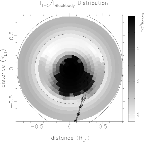
Figure 6: Left: The azimuthally averaged intensity distributions $I(T,\Sigma)$ (open circles) and $I_{BB}(T)$ (filled triangles) for comparison with error bars representing the scatter in each annulus. The dashed line at 0.53 $R_{\SS L1}$ indicates the size of the disc. Right: The ratio $I_{T,\Sigma}/I_{BB}$ as a grey-scale plot. The solid line represents the Roche-lobe, the dashed circular line the size of the disc and the dotted lines ballistic stream trajectories for mass ratios $0.19\pm 50$%. The secondary Roche lobe is at the bottom, outside the plotted region. See text for further explanation.

Fig. 3 shows the averaged quiescence light curves together with the final fit ($\chi^{2}=2.5$) for a distance of 145 pc. While the overall profiles are reproduced, the fits deviate in detail from the observed light curves. This is mainly due to flares and flickering, e.g. at phases $-0.135$ and 0.13. The U-band and B-band light curves are fitted best, which means the Balmer jump is quite well reproduced. The residuals of the R-band light curve are worst, most likely due to the lack of line emission, particularly H$\alpha$, in our model spectrum. This agrees with the negative residuals at mid-eclipse and the too shallow model light curve.

Further deviations, e.g. in disc ingress and egress, are probably due to the simplicity of the spectral model used. Keeping in mind that all light curves are fitted simultaneously, we would be rather surprised that such a simple spectral model fits the data so well. A future application of a more sophisticated, more realistic model would probably give a better reproduction of the observed light curves.

3.5 The reconstructions

The reconstructed temperature and surface density distributions are displayed in Fig. 5. In the centre the temperature reaches values up to nearly 15 000 K. It is fairly constant in the intermediate regions with a characteristic separation into a hot area with $T\sim 10\,500$ K and a cooler region with $T\sim 7500$ K. Towards the disc edge it drops linearly. The surface density rises from the central parts to the disc edge from values around 0.02 to 0.03 g cm^-2.

As pointed out in VHH, it is essential to study the behaviour of the spectral model in the given parameter space, before one can interpret the reconstructed maps. The easiest disc parameter to estimate is the disc size. We just need to look at the intensity distribution derived from the T-$\Sigma$ distributions, especially in the red filter. Since the R-band light curve is fitted worst, however, we would rather consider the V-band light curve in the present case. At a radius of 0.56$R_{\SS L1}$ the V-band intensity drops to about 1.5% of the maximum (i.e. the white dwarf intensity) and the distributions are to smoothed out due to the maximum entropy constraint. We therefore expect the disc edge to be between $0.507R_{\SS L1}$ and $0.56R_{\SS L1}$, i.e. at $0.53\pm 0.03R_{\SS L1}$. This disc radius is compatible with being smaller than the 3:1 resonance radius $R_{3:1}=0.68R_{\SS L1}$ (for $q=0.19$, Warner 1995), however, significantly smaller than Steeghs et al.’s (2001) radius of $1.1R_{\SS L1}$ (probably truncated due to tidal interactions to somewhere below 1$R_{\SS L1}$). Our disc radius describes the disc emitting continuum emission, while Steeghs et al.’s disc the line emission. It is possible that the chromosphere of the accretion disc extends to larger radii than 0.56$R_{\SS L1}$, however, there is no indication (e.g. precession of the disc) that the quiescent disc is larger than 0.68$R_{\SS L1}$. We rather suggest that the disc as observed by Steeghs et al. was affected by the immediately preceeding outburst.

When we compare the disc intensity $I(T,\Sigma)$ (averaged over azimuth and wavelength) with the black body intensity derived from the temperature distibution alone $I_{BB}(T)$ (Fig. 6), we see in which parts the disc resemble black body emitters. In the inner part of the disc the two distributions are nearly identical and the ratio $I_{T,\Sigma}/I_{BB}$ is very close to unity, i.e. the disc is nearly optically thick in the central region up to a radius of about $0.15R_{\SS L1}$. Towards the edge the disc become more and more optically thin or the temperature inversion in the chromosphere becomes more and more dominant.

The grey-scale plot in Fig. 6 also shows that the nearly optically thick region extends towards the region where the bright spot is expected, i.e. where the accretion stream from the secondary hits the accretion disc. In this impact region the disc material will have a higher density compared with regions with the same radius but different azimuth. However, the bright region extends also towards smaller azimuths, i.e. spreads against the flow of matter in the disc.

Figure 7: Averaged temperature (left) and surface density (right) distributions. The error bars indicate the reliability of the reconstructed parameter values. At small radii the disc is opticlly thick and we can only give lower limits for the surface density, indicated by triangles.

For a more quantitative analysis of the derived parameters, we plot the averaged parameter distributions in Fig. 7 with error bars according to a study of the spectral model. The error bars are derived as follows: Similar to the study in VHH, we calculated the spectrum for the averaged parameter pair ($T$,$\Sigma$) at a given radius, calculated spectra for a number of parameter pairs ($T+\Delta T$, $\Sigma+\Delta\Sigma$) around that parameter pair and determined the deviation of the spectra in terms of the $\chi^{2}$. The error bars include the temperature and surface density range for a $\chi^{2}$ of 3 for the given parameter pair. Small error bars indicate a high sensitivity of the spectrum to the parameter, while large error bars mean only little variation in the spectrum in the given parameter range, e.g. in the optically thick range the surface density would have an infinitely large error bar.

The error bars given in the averaged distributions (Fig. 7) are good estimates for the error bars that should be attached to the values in the original distribution (Fig. 5). They are omitted in Fig. 5 mainly for clarity of the plot, but partly also because it would suggest an exact estimate of the error bars.

We split the intermediate part of the disc (radii 0.2 to 0.5$R_{\SS L1}$) into an “upper” and a “lower” branch. The upper branch corresponds to the bright spot region, where the disc is nearly optically thick, the lower to the other parts of the disc.

The temperature is within the disc radius very well constrained. In contrast, the surface density values are partly much less well defined. The bright spot region has large error bars, because it is nearly optically thick. At small radii the disc is optically thick and therefore we can only give lower limits for the surface density $\Sigma$. However, the true values of $\Sigma$ can be very different from the given lower limits.

The temperature drops with radius as expected. It reaches about 13 000 K in optically thick, inner part of the disc and drops to about 6 000 K at the disc edge. The optically thick bright region has temperatures around 10 500 K while the other regions with identical radius have temperatures between 9 000 K and 6 500 K. These temperatures are significantly lower than those quoted by Berriman et al. (1986) of 20 000 K.

The surface density most likely increases with radius (as suggested by Fig. 5) or could be roughly constant, considering the partly large error bars in Fig. 7. (However, there is a clear distinction between the bright spot region and the rest of the disc.) Such a $\Sigma(r)$ distribution is compatible with theoretical calculations by Ludwig, Meyer-Hofmeister & Ritter (1994) and Cannizzo, Gosh & Wheeler (1982), but contradictory to Meyer & Meyer-Hofmeister’s (1982) calculations. Since the critical surface density distributions within the disc instability model show an increase of $\Sigma_{\mbox{\tiny crit}}$ (e.g. Cannizzo & Wheeler 1984) we would rather expect that the actual $\Sigma(r)$ distribution also increases with radius. However, as we see later (Section 4.4), these surface densities probably describe only the chromosphere of the disc.

3.6 The white dwarf

Using white dwarf spectra, the white dwarf temperature was reconstructed to 19 600 K using log g=8 white dwarf spectra. For the geometry we used only the “upper” half of the white dwarf, i.e. $0.25+(90^{\circ}-83.3^{\circ})/360^{\circ}=0.269$ of the total spherical surface. In the case that the disc is disrupted in the central part (i.e. if V2051 Oph is an intermediate polar) we would see more of the whole white dwarf and reconstruct a lower temperature. In case the white dwarf were fully visible the temperature would drop to 15 000 K. On the other hand, an accretion curtain may also hide part of the white dwarf surface, making it difficult to determine an exact value for the white dwarf temperature.

We estimated the error of the white dwarf temperature $T_{wd}$ by checking how the light curve fit changes with different values of $T_{wd}$ if we keep the disc parameters as reconstructed. This gives us an error of about 1 000 K. However, the error in $T_{wd}$ is linked to the error in the distance. Taking this into account, the total error is rather 2 000 K.

The geometry we used does not specifically set a location or size of a boundary layer. However, if such a boundary layer is present and emitting in the observed passbands, the emission should either be reconstructed in the innermost ring around the white dwarf or be hidden in the white dwarf emission. That we do not see a specific boundary layer emission in the innermost ring of the disc either means that the white dwarf temperature is overestimated or that there is no boundary layer (see Section 4.6).

Steeghs et al. (2001) and Catalan et al. (1998) both find a white dwarf temperature of 15 000 K. However, since both do not state which distance value they used a direct comparison to our value is not possible. Assuming they used a similar distance, this would mean that we might see part of the “lower hemisphere”. However, this is doubtfull, since the disc is optically thick near the white dwarf and should occult the “lower” half of the compact source. If the boundary layer were hidden in the white dwarf emission, Steeghs et al. and Catalan et al. should have faced the same problem.

The reconstructed value is close to typical values of white dwarf temperatures, but somewhat higher than in the similar objects HT Cas, OY Car and Z Cha of around 15 000 K (Gänsicke & Koester 1999 and references therein). This might be connected to the somewhat different system parameters as shown in Tab. 5.

3.7 The uneclipsed component

Table 4: The reconstructed fluxes (in mJy) for the uneclipsed component $F_{un}$ as well as a M4.5 and M5.5 main sequence star, $F_{\mbox{M4.5}}$ and $F_{\mbox{M5.5}}$, respectively.

Filter	$F_{un}$	$F_{\mbox{M4.5}}$	$F_{\mbox{M5.5}}$
U	0.59
B	0.44
V	0.00	0.09	0.01
R	0.66	0.30	0.07

Apart from the disc parameters we also reconstructed an uneclipsed fraction of the light curve (Table 4). For the reconstruction of this component, we do not need to assume any spectral model. It is simply any uneclipsed flux in the given filter and free for any interpretation.

Since the uneclipsed spectrum might be generaly underestimated, the B-flux overestimated (Vrielmann & Baptista 2002) and since the errors in the uneclipsed component particularly in the V and R-band filters are rather large (Vrielmann et al. 2002), we cannot derive much physics out of this component. All we can say is that the uneclipsed component is compatible with a M5 main sequence star (using Baptista et al.’s mass and radius and Kirkpatrick & McCarthy 1994 tables for main sequence stars, see Table 4) plus an optically thin component emitting particularly in the U-band and R-band, e.g. a chromosphere and/or disc wind.

Evidence for a disc wind comes from the fact that the blueshifted Doppler emission component of all emission lines is always brighter than the redshifted component (Kaitchuck et al. 1994, Honeycutt, Kaitchuck & Schlegel 1987). Even though Steeghs et al. (2001) claim to find a reversal of this asymmetry for H$\alpha$ (i.e. the red peak is stronger) we cannot see this in their gray-scale plot: their Fig. 1 shows the blue wings stronger at all plotted phases (-0.3 to 0.1) except during part of the eclipse. Furthermore, the eclipse is shorter and shallower in the blue peak than in the red peak, indicating that the origin of the blue emission is spatially focused and only partly eclipsed, e.g. like a collimated wind (or jet) above the disc. And although in Warner & O’Donoghue’s (1987) spectrum the red peak is higher, the blue peak is slightly broader, indicating that the additional emission in the blue wings has rather high velocities.

3.8 Derived parameters

From the reconstructed parameter distributions we can calculate several further parameters, like the effective temperature, the disc scale height and the viscosity. These parameters are more descriptive of the disc than the gas temperature and surface density. The disc size and effective temperature can in particular be determined more accurately than the originally reconstructed ones, because they rather depend on the intensity distributions corresponding to the original reconstructions than on the reconstructed parameters themselves. However, in general the derived values are only as certain as the originally reconstructed values on which they are based and one has to be careful in interpreting the resulting derived parameter values. One must also keep in mind, that these parameters might only describe the hot chromosphere, not the entire disc (see Section 4.4). Furthermore, it is difficult estimating an error of the derived parameters without extremely time consuming Monte-Carlo type calculations.

3.8.1 The effective temperature and mass accreion rate

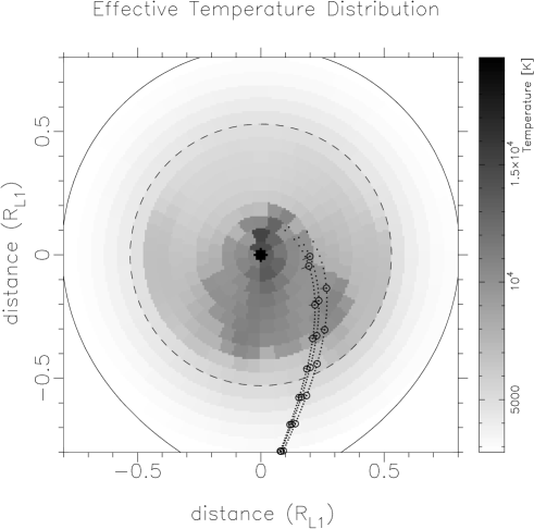
Figure 8: Left: The radial effective temperature distribution in quiescence. The underlying dotted lines are theoretical steady state temperature distributions for $\log\dot{\cal M}=13$ to 18, the one for $\dot{\cal M}=10^{16}$gs^-1is drawn solid for reference. The dashed-dotted lines indicates the critical effective temperature $T_{{\mbox{\scriptsize eff}},{\rm A}}$ according to Ludwig, Meyer-Hofmeister & Ritter’s (1994) critical mass accretion rate $\dot{\cal M}_{\rm A}$. Right: The spatial distribution of the effective temperature as a grey-scale plot. The solid line represents the Roche-lobe of the primary, the dashed line (in both plots) the disc size and the dotted lines ballistic accretion stream lines for mass ratios 0.19 $\pm$ 50%. The secondary Roche lobe is at the bottom, outside the plotted region.

From the temperature and surface density distributions we can calculate the spatially resolved effective temperature $T_{\mbox{\scriptsize eff}}$ distribution in the disc (Fig. 8). $T_{\mbox{\scriptsize eff}}$ is calculated from the intensity $I_{\nu}(T,\Sigma)$ as

$$\pi\int I_{\nu}(T,\Sigma)\,\,d\nu=\sigma T_{\mbox{\scriptsize eff}}^{4}$$ (3)

with $\sigma$ the Stefan-Boltzmann constant. In practice, $I_{\nu}$ is summed numerically over a large frequency range $\nu$. Equation 3 shows that $T_{\mbox{\scriptsize eff}}$ does not directly depend on the reconstructed values $T$ and $\Sigma$, but rather on the intensity derived from them. Since the intensity distribution directly translates into the observed fluxes which are as good as the fit to the light curves suggests, the effective temperature is more reliable than the surface density values and rather comparable to the certainty of the reconstructed temperature values.

The main part of the disc has a mass accretion rate of between $\dot{\cal M}=1\times 10^{15}$ gs^-1 to $\dot{\cal M}=1\times 10^{17}$ gs^-1 ($1.6\times 10^{-11}{\cal M}_{\odot}$ yr^-1 to $1.6\times 10^{-9}{\cal M}_{\odot}$ yr^-1). However, the distribution is split into two parts of higher and lower temperatures. As the grey-scale plot in Fig. 8 shows, the higher temperatures are associated with the bright spot region, or more general to the region between the two stars, i.e. the same region that is nearly optically thick. The remainder of the disc is cooler.

This situation is understandable in terms of the mass accretion rate involved. At the bright spot the mass transfer is highest, reaching $1\times 10^{17}$ gs^-1, because of the impact of the gas stream from the secondary. In the remaining disc, the mass accretion rate is determined solely by the viscosity. In the region $180^{\circ}$ away from the gas stream the mass accretion rate drops to values around $3\times 10^{15}$ gs^-1.

Fig. 8 also shows the theoretical critical effective temperature $T_{{\mbox{\scriptsize eff}},{\rm A}}(R)$ derived from the critical mass accretion rate $\dot{\cal M}_{\rm A}(R)$ as given by Ludwig et al. (1994), indicating whether the disc should undergo outbursts (see Section 4.5).

3.8.2 The disc mass

The disc mass can be estimated from the surface density, however, only with a certainty that the reconstructed surface density values allow. For the disc within a radius of 0.53$R_{\SS L1}$ we derive a mass of $7.7\times 10^{19}$ g or $3.9\times 10^{-14}{\cal M}_{\odot}$. This value has to be treated with some caution. The disc is nearly optically thick in the centre, i.e. for that region we rather derive a minimum value of $\Sigma$ and therefore of the disc mass. In the outer parts of the disc the surface density might vary by up to a third of the reconstructed value for $\Sigma$. The error in the disc mass therefore must be set to roughly 50% of the derived value.

According to Frank, King & Raine (1992) the mass in the disc at any one time is $M_{disc}{\textstyle{\;\lower 3.01385pt\hbox{$<$}\;\atop\raise-0.3014pt\hbox{$\sim$}}}10^{-10}{\cal M}_{\odot}\alpha^{-4/5}\dot{\cal M}^{7/10}_{16}$, where $\dot{\cal M}_{16}$ is the mass accretion rate in units of $10^{16}$ gs^-1 and $\alpha$ the viscosity coefficient determined by $\nu=\alpha c_{s}H$, where $\nu$ is the viscosity, $c_{s}$ the sound speed and $H$ disc thickness. So, unless $\alpha$ reaches unreasonably high values of the order of $10^{4}$ or the underlying disc is extremely massive, Frank et al.’s condition is well fulfilled.

3.8.3 The disc scale height

Figure 9: The radial distribution of the disc scale height. The circle at a disc radius of 0$R_{\SS L1}$ represents the radius of the white dwarf and illustrates how geometrically thin the disc is. The scale of the radius (x-axis) would have to be multiplied with a factor of $2.9\times 10^{10}$ cm $R_{\SS L1}^{-1}$ to be translated into the same units as the scale height.

We can estimate an equilibrium scale height of the disc (or rather its chromosphere, Fig. 9). The value of $H/R$ ranges around 0.01, i.e. the opening angle of the disc is about $0^{\circ}_{\raisebox{1.80835pt}{\hskip 0.35002pt.}}6$ with a scatter of $0^{\circ}_{\raisebox{1.80835pt}{\hskip 0.35002pt.}}1$ and the disc has a scale height of only 1/4 white dwarf radii at the disc radius. The error on the values of H are fairly small (less than 1%), as this parameter only depends on the square-root of the temperature. This validates our assumption of a geometrically thin disc. Up to a radius of $0.4R_{\SS L1}$ the disc has a slight concave shape with the opening angle ranging between $0^{\circ}_{\raisebox{1.80835pt}{\hskip 0.35002pt.}}4$ and $0^{\circ}_{\raisebox{1.80835pt}{\hskip 0.35002pt.}}85$.

However, this disc scale height is calculated with the assumption of an iso-thermal vertical ($z$-)structure of the disc. Realistic calculations of the disc photosphere lead (for mass accretion rates estimated in this paper) to disc opening angles of about 3 degrees in addition to the underlying disc with unknown, but most likely non-negligible opening angle. In an as high-inclination system as V2051 Oph this should lead to significant front-back asymmetries in the disc emission (however, opposite to what we observe, see Section 4.3).

3.8.4 The disc viscosity

Using the formula

$$\frac{3}{2}\Omega_{K}\alpha PH=\int F_{\nu}d\nu$$ (4)

where $\Omega_{K}=\sqrt{GM_{W}/R}$ is the Keplerian angular velocity, $P$ the gas pressure (calculated according to the perfect gas law: $T=\mu m_{H}P/\rho k$, with $T$ the temperature, $\mu$ the ionization coefficient, $m_{H}$ the mass of the hydrogen atom, $\rho$ the density and $k$ the Boltzmann’s constant), $H$ again the disc scale height and $F_{\nu}$ the flux at frequency $\nu$, we can determine the viscosity parameter $\alpha$ (Shakura & Sunyaev 1973) throughout the disc. Typical values of $\alpha$ in a quiescent disc should lie around 0.01 (e.g. Smak 1984).

The derived values are very high (between 50 and 900) and incompatible with current accretion disc models. A very similar situation arises in the dwarf nova HT Cas (Wood, Horne & Vennes 1992, Vrielmann 1997, Vrielmann et al. 2002). We see a need to explain these high values.

We suggest that the structure of the disc is such, that we do not see the entire disc. For example, in the case that part of the disc is obscured or outshined by a hot chromosphere, the gas density is higher than calculated and $\alpha$ would be lower. In Section 4.4 we propose a model of the disc, which could – in principle – explain the observations. However, only concrete theoretical calculations of such a scenario can show if such a model is indeed applicable.

4 Summary & Discussion

4.1 The distance

We derived a new distance to V2051 Oph of $146\pm 20$ pc using the Physical Parameter Eclipse Mapping (PPEM) method, assuming that the true distance would lead to the smoothest reconstruction. Our result is compatible with those of Watts et al. (1986) and Berriman et al.’s (1986). This agreement and a few others others (Vrielmann 2001) support the applicability of PPEM to derive distances even when we use a very simple spectral model for the disc emission. However, the method certainly has to be applied to a large number of systems and compared to independent distance estimates before it can be considered established.

4.2 The radial light distribution of the accretion disc

We applied the PPEM to a quiescent UBVR data set. The disc appears nearly optically thick inside a radius of about $0.2R_{\SS L1}$ and in the region where the bright spot is expected (up to a radius of about $0.4R_{\SS L1}$), while outside these regions the disc is optically thin or shows an increasing dominance of a temperature inversion in the disc chromosphere. This agrees with Tylenda (1981) and Watts et al. (1986) in general, although not in detail.

Tylenda’s (1981) calculations show that a disc with a mass accretion rate of $10^{16}$gs^-1 is optically thin in the outer parts at radii larger than $1.2\times 10^{10}$cm (for V2051 Oph this corresponds to 0.42$R_{\SS L1}$). Since the accretion disc of V2051 Oph has a radius of about $1.55\times 10^{10}$cm ($\sim 0.53R_{\SS L1}$) this transition zone lies well within the disc radius, however, is incompatible with ours.

Using the equivalent width (EW) of the Balmer emission lines during an orbit, Watts et al. found the radius of the transition between the dominance of optically thin over thick regions to be at a radius of $0.16\pm 0.02$a (= $0.24\pm 0.03R_{\SS L1}$). Their value lies inbetween our radius of the optically thick part of the disc (0.2 and 0.4$R_{\SS L1}$), because their method implies axisymmetry of the accretion disc emission.

The fact that emission lines of V2051 Oph have broad wings that originate at radii $R<0.2R_{\SS L1}$ (if the disc is Keplerian, see also also Section 4.6) must mean that they originate from a (chromospheric) layer above the disc (see Section 4.4).

4.3 The bright region in the accretion disc

Why does the disc show the bright region between $-30^{\circ}$ and $+60^{\circ}$ (Fig. 8) as well as a high temperature ridge from the white dwarf to the edge of the disc at an azimuth of about $-10^{\circ}$?

This bright region is associated with enhanced emission and therefore not explicable as a back-front assymetry as expected for a disc with a significant, underestimated (or neglected) opening angle. The latter would lead to an enhancement in the “back” part of the disc, i.e. at azimuths around $\pm 180^{\circ}$.

The bright spot region appears to be nearly optically thick in quiescence and slightly preceding the theoretical position in the direction of motion in the disc. However, one would rather expect the bright spot region to extend from the impact area into the direction of motion in the disc. Even though this bright region might be only temporary and is only derived using observation near the eclipse, we discuss its possible origin.

We carefully checked if the reconstructed location of the bright spot region is caused by an errornous ephemeris, but must conclude that this cannot be the case. This means, if the feature is real, there must be a physical reason for this unexpected disc structure. Since the secondary plays only a minor role in V2051 Oph, as its contribution is small compared to the disc, it cannot be responsible for illumination of the disc.

The high temperature ridge may indicate that the disc is warped and the ridge at azimuth $-10^{\circ}$ maximally illuminated by the white dwarf. The azimuths $+170^{\circ}$ would then not be illuminated by the white dwarf. Since the data we used for the PPEM analysis cover only the phases $\pm 0.15$ we never see the outer regions of the disc around azimuth angles $\pm 180^{\circ}$ leading to low temperatures in our reconstructions. This warp would, however, have to be fixed in the rotating frame to be so prominent in the maps derived from averaged light curves. But calculations by Schandl & Meyer (1994) who propose coronal winds as the cause of the warp, show a precession of the disc, making the warp model unlikely.

Another possible scenario is a bulge in the disc similar as the one proposed by Buckley & Tuohy (1989) at the location of the impact region. This bulge could illuminate the disc area around azimuth angle 0. How the high temperature ridge can be formed is unclear and it would be interesting to analyse multi-colour observations of other epochs to see if this feature is stable.

Kaitchuck et al. (1994) calculated Doppler images of the emission lines H$\beta$ and He I $\lambda$4471. They find that the leading side of the disc is brighter than the trailing side. The location of their bright area does not coincide with our bright region. However, they investigate the location of the line emission, which should be minimal in an optically thick area and could therefore correspond to the bulge itself or the region ahead of the bulge (i.e. at even larger azimuths) as proposed by Hoard et al. (1998) for the nova-like UU Aqr. Their disc model involves an emitting impact spot with a trail of optically thin material along the edge of the disc.

The size and location of the bright region will be correlated with the mass accretion rate $\dot{\cal M}$, since the latter determines the disc size. It would therefore be interesting to study V2051 Oph at various times during high and low states. For example, the variability in $\dot{\cal M}$ may also be the reason, why Watts et al. (1986) could not detect the $s$-wave (produced by a bright spot), while it was clearly present in Honeycutt, Kaitchuck & Schlegel’s (1987) data and might indicate a variability in the bulge.

4.4 The vertical disc structure

We propose that the disc itself must have a structure as follows, and similar to the disc structure suggested for HT Cas (Vrielmann 2001, Vrielmann et al. 2002): The disc consists of a cool, optically thick layer with a hot chromosphere on both sides of the disc. This chromosphere is nearly optically thick at small radii, but optically thin for most of the disc. What we see of the disc is mainly the hot chromosphere and little from the cool layer underneath, therefore the temperature and in particular the surface density are descriptive only of the chromosphere. Such a model was first proposed by Wood et al. (1992), Menou (2002) has done some more recent theoretical work on it.

This disc model resolves in the confusion about the optical depth of the disc and subsequently our derived values of $\alpha$. On the one hand, the disc instability model (e.g. Ludwig et al. 1994, Faulkner et al. 1983, Smak 1982) predicts that the surface density values should lie between 10 and 100 g cm^-2 for $\alpha$’s between 0.1 and 1 and even at larger $\Sigma$’s for smaller $\alpha$’s. This means that the disc must have a massive, optically thick component.

On the other hand we see line emission from the disc during quiescence, rise and decline of an outburst (e.g. Hessman et al. 1984) which indicates that there must be an optically thin component during these phases in the outburst cycle. Our derived surface density values in the disc re-confirms that the optically thin source (or more correctly, the non-black body source) is associated with the disc.

The sandwich model elegantly combines both the observational findings (optically thin material) and the theoretical predictions (optically thick disc). It also explains why we find such high values of $\alpha$: Since we see mainly the contribution from the hot chromosphere, the surface densities describe only the upper layers of the accretion disc. The true surface densities ($\Sigma$) must be much larger, of the order 10 to 100 g cm^-2. A simple estimate confirms that values around 100 g cm^-2 for $\Sigma$ lead to $\alpha$’s in the expected range of 0.01 to 1. Thus, we have found a simple explanation, why we derive such high values for $\alpha$ without discarding the accretion disc models or our PPEM method: Using the surface density of the chromosphere alone and assuming it to describe the whole accretion disc leads to high values of the viscosity parameter $\alpha$.

The proposed chromosphere must extend to such heights above the orbital plane that part of it is never eclipsed, i.e. near the white dwarf it must reach farther up than about $0.2R_{\SS L1}$ or $0.085R_{\odot}$ or about $8R_{wd}$ (see Section 3.7). This chromosphere should also be the site of the observed emission lines which would be produced by non-radiative energy dissipation, analogous to a stellar chromosphere (Horne & Saar 1991).

A more extensive explanation of the vertical disc structure is given in Vrielmann et al. (2001) for the similar system HT Cas.

4.5 The mass accretion rate

Similar to results of Watts et al. (1986), the quiescent mass accretion rate appears in large parts of the disc to be somewhat higher than or around the critical values given by Ludwig et al. 1994 or Watts et al. of $\sim 4.6\times 10^{-11}{\cal M}_{\odot}$ yr^-1 (for $K_{1}=111$km s${}^{-}1$). The latter derived a similar accretion rate for V2051 Oph as we of $\sim 1.3\times 10^{-10}{\cal M}_{\odot}$ yr^-1 compared to our $1.6\times 10^{-11}{\cal M}_{\odot}$ yr^-1 to $1.6\times 10^{-9}{\cal M}_{\odot}$ yr^-1. Fig. 8 shows that specifically the bright spot and inner, hot regions ($R<0.1R_{\SS L1}$) have higher temperatures than the critical values $T_{{\mbox{\scriptsize eff}},{\rm A}}(R)$.

Since V2051 Oph shows outbursts, and probably very infrequently, the effective temperature should not lie so close to or even above the critical $T_{{\mbox{\scriptsize eff}},{\rm A}}(R)$, but rather far below (e.g. Warner 1995). Berriman et al. (1986) also found that V2051 Oph’s disc is too hot to undergo the disc instability cycle. The only known outbursts around the time of our observations (June 1983) were the ones in April 1982 and in May 1984. V2051 Oph has infrequent observed outbursts and a typical outburst cycle of about a few years (VSNET observations). So the disc is unlikely to have been affected by a rise to or decline from outburst. A similar situation occurs in HT Cas (Vrielmann et al. 2002), a dwarf nova with reportedly infrequent outbursts. At the moment, we have no solution for this problem. Until another explanation is found, we must assume that either our mass accretion rates are errorneous or that it is sufficient if part of the disc has effective temperatures below the critical value.

We would recommend a study of this object throughout a quiescent cycle in order to check variations in the mass accretion rate, especially before the onset of an outburst and during low states ($B\sim 16.2$, Baptista et al. (1998), compared to $B\sim 15$ (WO). Interestingly, HT Cas, a similar dwarf nova, also shows variations during quiescence (Robertson & Honeycutt 1996) with fluctuations of about 1.5 mag.

Furthermore, it would be very desirable to get an independent distance estimate. If the distance were significantly smaller than our estimate, the effective temperatures and mass accretion rates would be reconstructed to smaller values. However, this will not solve the problem, because an (unlikely) reduction of a factor two in distance will only lead to a small reduction in effective temperatures to $0.5^{1/4}T_{\mbox{\scriptsize eff}}=0.84T_{\mbox{\scriptsize eff}}$ and therefore to a small change in $\dot{\cal M}$.

4.6 Is V2051 Oph an intermediate polar?

While it is clear that V2051 Oph shows typical features of a SU UMa system (outbursts and super outbursts), it is not clear, whether the white dwarf has a small magnetic field.

An intermediate polar should show a disrupted inner disc in the PPEM maps, unless the inner disc radius is too small. We do not see any indication for a hole, except for a flattening of the effective temperature towards the white dwarf. Only a very tiny hole could be hidden due to the MEM smearing, as tests of the PPEM method show. However, estimating the line width at phase 0.51 of H$\alpha$ in WO’s Fig. 10, we yield $\sim 77$Å, i.e. the disc material at the inner disc edge has a velocity of about 1777 kms^-1. For a Keplerian disc this corresponds to an inner disc radius of $3.3\times 10^{9}$ cm $=0.11R_{\SS L1}$. More recent, yet unpublished data of V2051 Oph suggest line wings extending to about 2530 kms^-1, corresponding to an inner disc radius of 2.3 white dwarf radii. Quiescence data of Watts et al. (1986) also show line wings of H$\beta$ and H$\gamma$ extending to maximally 2500 kms^-1 (corresponding to $R_{in}=0.06R_{\SS L1}=2.4R_{wd}$).

Steeghs et al. (2001) find much broader line wings. Both spectra sets were taken during decline from outburst which means that the emission lines should have been affected in the same way. Since the intensity in the outer line wings is extremely low ($<3\%$ for $v<-2500$ kms^-1; red wing affected by He line, Fig. 3 of Steeghs et al.), broad shallow wings could – in principle – be lost in the noise of the above mentioned spectra, however, no such line profiles as observed by Steeghs et al. can be hidden in those spectra. Only the blue wing of H$\beta$ can be measured reliably, which will be enhanced by the disc wind, a possible explanation for Steeghs et al.’s broad line profile.

The fact that we do not see a hole in the reconstructed disc means either, there is none, it is extremely small, or it could be hidden by accretion curtains.

X-ray observations (Holcomb, Caillault & Patterson 1994, van Teeseling, Beuermann & Verbunt 1996) and lack of circular polarisation (Cropper 1986) data do not contradict the intermediate polar model with a very weak magnetic field of 1 MG or less, as expected for intermediate polars.

Thus, if V2051 Oph is indeed an intermediate polar, its white dwarf must have a very weak magnetic field which allows to disc to be disrupted with an inner disc radius of $R_{in}<0.1R_{\SS L1}=4.2R_{wd}$. At present we cannot distinguish between such a low field intermediate polar and a dwarf nova. However, the variable hump and irregular occurance of strong flares as observed by WO and Berriman et al. 1986 might indicate a flaring accretion curtain which lights up during inhomogeneous accretion. Warner & Woudt (2002) propose a model for V2051 Oph in which the spinup of the magnetic field lines of a small field on the white dwarf temporarily creates such a small hole of a a few tenths larger than the white dwarf radius. Their model applies to a disc on decline from outburst. During quiescence they expect the hole to be even slightly larger. If this hole is present and persisting long enough, accretion curtains can develop, leading to the observed flares.

Simultaneous multi-colour observations at different epochs and high resolution spectroscopy are very desirable in order to solve the mystery of V2051 Oph’s nature.

4.7 Comparison to similar objects

V2051 Oph has a similar orbital period as OY Car, Z Cha and HT Cas and since all of them are SU UMa system, showing super outbursts inbetween their normal ones, one would expect to find some similarities among these systems. However, the light curve of V2051 Oph seems to vary a lot more than that of the other three systems, especially in terms of the presence and location of the (orbital) hump, flickering and flaring.

The eclipse light curve of OY Car (Vogt et al. 1981, Wood et al. 1989, Rutten et al. 1992, Horne et al. 1994) is remarkably stable over more than a decade and even close to a super outburst (Hessman et al. 1992). A similar consistency in the appearance is shown by HT Cas (Berriman et al. 1987, Horne et al. 1991, Robertson & Honeycutt 1996) and Z Cha (Wood et al. 1986, Marsh et al. 1987, Robinson et al. 1995). OY Car and Z Cha even show text book light curves of eclipsing dwarf novae in which the orbital hump and the ingress and egress phases of the white dwarf and the bright spot can be very well distinguished and explained in the standard Roche model. HT Cas, on the contrary, has never been observed to show an orbital hump.

Table 5: System parameters of V2051 Oph and similar SU UMa type dwarf novae in comparison.

Parameter	V2051 Oph	HT Cas	OY Car	Z Cha
$P\hskip 4.30554pt[h]$	1.50	1.77	1.51	1.79
$i$	$83^{\circ}_{\raisebox{1.80835pt}{\hskip 0.35002pt.}}3\hskip 4.30554pt\pm\hskip 4.30554pt1^{\circ}_{\raisebox{1.80835pt}{\hskip 0.35002pt.}}4$	$81^{\circ}_{\raisebox{1.80835pt}{\hskip 0.35002pt.}}0\hskip 4.30554pt\pm\hskip 4.30554pt1^{\circ}_{\raisebox{1.80835pt}{\hskip 0.35002pt.}}0$	$83^{\circ}_{\raisebox{1.80835pt}{\hskip 0.35002pt.}}3\hskip 4.30554pt\pm\hskip 4.30554pt0^{\circ}_{\raisebox{1.80835pt}{\hskip 0.35002pt.}}2$	$81^{\circ}_{\raisebox{1.80835pt}{\hskip 0.35002pt.}}7\hskip 4.30554pt\pm\hskip 4.30554pt0^{\circ}_{\raisebox{1.80835pt}{\hskip 0.35002pt.}}13$
$q$	$0.19\hskip 4.30554pt\pm\hskip 4.30554pt0.03$	$0.15\hskip 4.30554pt\pm\hskip 4.30554pt0.03$	$0.102\hskip 4.30554pt\pm\hskip 4.30554pt0.003$	$0.1495\hskip 4.30554pt\pm\hskip 4.30554pt0.0035$
${\cal M}_{wd}\hskip 4.30554pt[{\cal M}_{\odot}]$	$0.78\hskip 4.30554pt\pm\hskip 4.30554pt0.06$	$0.61\hskip 4.30554pt\pm\hskip 4.30554pt0.04$	$0.685\hskip 4.30554pt\pm\hskip 4.30554pt0.011$	$0.54\hskip 4.30554pt\pm\hskip 4.30554pt0.01$
${\cal M}_{r}\hskip 4.30554pt[{\cal M}_{\odot}]$	$0.15\hskip 4.30554pt\pm\hskip 4.30554pt0.03$	$0.09\hskip 4.30554pt\pm\hskip 4.30554pt0.02$	$0.070\hskip 4.30554pt\pm\hskip 4.30554pt0.002$	$0.081\hskip 4.30554pt\pm\hskip 4.30554pt0.003$
$\dot{\cal M}$   [gs-1]	$1\times 10^{17}$	$5\times 10^{15}$	$4\times 10^{15}$	$4\times 10^{15}$

$\dot{\cal M}$: Mass accretion rate at the disc radius (disc edge) or into the bright spot

References: V2051 Oph: Baptista et al. (1998), HT Cas: Horne et al. (1991), Vrielmann et al. (2002, $\dot{\cal M}$),

OY Car: Wood et al. (1989), Horne et al. (1994), Z Cha: Wood et al. (1986)

For comparison, we listed a few system parameters of these four objects in Tab. 5. While at first glance all parameters seem to be similar, closer inspection reveals that the secondary in V2051 Oph is about twice as massive as the secondaries in the other systems. Furthermore, also the mass accretion rate $\dot{\cal M}$ into the disc of V2051 Oph is larger by a factor of twenty or more than in the other systems (in OY Car and Z Cha $\dot{\cal M}$ was determined by Eclipse Mapping (Wood et al. 1989 using d=100 pc, Horne et al. 1994; Wood et al. 1986) and in HT Cas with the PPEM method (Vrielmann et al. 2002)).

The larger amount of variation of V2051 Oph could be induced by the larger mass accretion rate, being close to or above the theoretical limit. Even if the disc were rather patchy with a covering factor of maybe 50%, as proposed for HT Cas (Vrielmann et al. 2002), the mass accretion rate were still a factor of about ten or more larger than that of the other three dwarf novae. The larger mass of the secondary in V2051 Oph, could be the reason for the higher mass accretion rate, however, it is not fully understood, how $\dot{\cal M}$ is related to other system parameters. Furthermore, it is not clear, how the larger $\dot{\cal M}$ alone can cause the occational occurence of a hump. We therefore, cannot exclude the low-field intermediate polar model.

4.8 Concluding remark

Since V2051 Oph is usually too faint for amateur astronomers, monitoring of this object is difficult, but particularly interesting. Especially also the evolution of the disc during normal and low quiescent states and the percentage of time V2051 Oph spends in either state would be of immense interest.

References

- [1] Baptista R., Steiner J.E., 1993, A&A 277, 331
- [2] Baptista, R., Catalán, M.S., Horne, K., Zilli, D. 1998, MNRAS, 300, 233
- [3] Berriman, G., Kenyon, S., Bailey, J. 1986, MNRAS, 222, 871
- [4] Berriman, G., Kenyon, S., Boyle, C. 1987, AJ, 94, 1291
- [5] Bond, H. & Wagner R.L. 1977, IAU Circ. 304
- [6] Buckley, D.A.H., Tuohy, I.R. 1989, ApJ, 344, 376
- [7] Cannizzo, J.K., Wheeler J.C. 1984, ApJS, 55, 367
- [8] Cannizzo, J.K., Gosh, P., Wheeler J.C. 1982, ApJ, 260, L83
- [9] Catalan, M.S., Horne, K., Cheng, F.H., Marsh, T.R., Hubeny, I., 1998, ASP Conf. Series 137, Wild stars in the Old West, p. 426
- [10] Cropper, M. 1986, MNRAS, 222, 225
- [11] Frank, J., King, A., Raine D. 1992, “Accretion Power in Astrophysics”, Cambridge Astrophysics Series, Cambridge University Press, p. 81
- [12] Faulkner, J., Lin, D.N.C., Papaloizou, J. 1983, MNRAS, 205, 359
- [13] Gänsicke, B.T., Koester, D. 1999, A&A, 346, 151
- [14] Hessman, F.V., Robinson, E.L., Nather, R.E., Zhang, E.-H. 1984, ApJ, 286, 747
- [15] Hessman, F.V., Mantel, K.-H., Barwig, H., Schoembs, R. 1992, A&A, 263, 147
- [16] Hoard, D.W., Szkody, P., Still, M.D., Smith, R.C., Buckley, D.A.H. 1998, MNRAS, 294, 689
- [17] Holcomb, S., Caillault, J.-P., Patterson, J. 1994, AAS, 185, 2117
- [18] Honeycutt, R.K., Kaitchuck, R.H., Schlegel, E.M. 1987, ApJS, 65, 451
- [19] Horne K., 1985, MNRAS 213, 129
- [20] Horne, K., Saar, S.H. 1991, ApJ, 374, L55
- [21] Horne K., Wood J.H., Stiening R.F., 1991, ApJ, 378, 271
- [22] Horne K., Marsh, T.R., Cheng, F.H., Hubeny, I, Lanz, T. 1994, ApJ, 426, 294
- [23] Hubeny I., 1991, in IAU Colloq. 129, Structure and Emission Properties of Accetion Disks, eds. C. Bertout, S. Collin, J.-P. Lasota, J. Tran Thanh Van (Singapure: Fong & Sons), p. 227
- [24] Kaitchuck, R.H., Schlegel, E.M., Honeycutt, R.K., Horne, K., Marsh, T.R., White II, J.C., Mansperger, C.S. 1994, ApJS, 93, 519
- [25] Kirkpatrick, J.D., McCarthy, Jr, D.W. 1994, AJ, 107, 333
- [26] Kiyota, S., Kato, T. 1998, IBVS, No. 4644
- [27] Ludwig K., Meyer-Hofmeister E., Ritter H., 1994, A&A 290, 473
- [28] Marsh, T.R., Horne, K., Shipman, H.L. 1987, 225, 551
- [29] Meyer, F., Meyer-Hofmeister, E., 1982, A&A, 106, 34
- [30] Menou, K., 2002, in “The Physics of Cataclysmic Variables and Related Objects”, Göttingen, August 5-10, 2001, ed. B. Gänsicke, K. Beuermann, K. Reinsch, ASP conference series, in press
- [31] Robertson, J.W., Honeycutt, R.K., 1996, AJ, 112, 2248
- [32] Robinson, E.L., Wood, J.H., Bless, R.C., Clemens, J.C., Dolan, J.F., Elliot, J.L., Nelson, M.J., Percival, J.W., Taylor, M.J., van Citters, G.W., Zhang, E. 1995, ApJ 443, 295
- [33] Rutten, R.G.M., Kuulkers, E., Vogt, N., van Paradijs, J. 1992, A&A, 265, 159
- [34] Sanduleak, N. 1972, IBVS, No. 663
- [35] Schandl, S., Meyer, F. 1994, A&A, 289, 149
- [36] Shakura N.I., Sunyaev R.A., 1973, A&A, 24, 337
- [37] Shlosman, I., Vitello, P.A.J., Mauche, C.W. 1996, ApJ, 461, 377
- [38] Skilling J., Bryan R.K., 1984, MNRAS 211, 111
- [39] Smak, J. 1982, Acta Astr., 32, 199
- [40] Smak, J. 1984, PASP, 96, 5
- [41] Steeghs, D., O’Brien, K., Horne, K., Gomer, R., Oke, J.B. 2001, MNRAS, 323, 484
- [42] van Teeseling, A., Beuermann, K., Verbunt, F. 1996, A&A, 315, 467
- [43] Vrielmann, S. 1997, Ph.D. thesis, University of Göttingen
- [44] Vrielmann, S. 1999, in “Disk Instabilities in Close Binary Systems”, Kyoto, October 27-30, 1998, ed. S. Mineshige and J.C. Wheeler, Universal Academy Press, p. 115
- [45] Vrielmann, S. 2001, in “Astro Tomography”, Brussels, ed. D. Steeghs, H. Boffin, Lecture Notes in Physics, Springer Verlag, in press
- [46] Vrielmann, S., Baptista, R., 2002, submitted to AN
- [47] Vrielmann, S., Horne, K., Hessman, F.V. 1999, MNRAS, 306, 766 (VHH)
- [48] Vrielmann, S., Hessman, F.V., Horne, K. 2002, MNRAS, in press
- [49] Vogt, N., Schoembs, R., Krzeminski, W., Pedersen, H. 1981, A&A, 94, L29
- [50] Tylenda, R. 1981, Acta Astron., 31, 127
- [51] Warner, B. 1995, “Cataclysmic variable stars”, Cambridge Astrophysics Series, Cambridge University Press, p. 207
- [52] Warner, B. 1996, Ap&SS, 241, 263
- [53] Warner, B., Woudt, P.A. 2002, submitted to MNRAS
- [54] Warner, B., Cropper, M. 1983, MNRAS, 203, 909
- [55] Warner, B., O’Donoghue, D. 1987, MNRAS, 224, 733 (WO)
- [56] Watts, D.J., Bailey, J., Hill, P.W., Greenhill, J.G., McCowage, C.,Carty, T. 1986, A&A, 154, 197
- [57] Wood J.H., Horne, K., Berriman, G., Wade, R., O’Donoghue, D., Warner, B. 1986, MNRAS, 219, 629
- [58] Wood J.H., Horne, K., Berriman, G., Wade, R. 1989, ApJ, 341, 974
- [59] Wood J.H., Horne K., Vennes S., 1992, ApJ, 385, 294