Dark Halo Shapes and the Fate of Stellar Bars

Abstract

We investigate the stability properties of trajectories in barred galaxies with mildly triaxial halos by means of Liapunov exponents. This method is perfectly suitable for time-dependent 3-D potentials where surfaces of sections and other simple diagnostics are not applicable. We find that when halos are centrally-concentrated most trajectories starting near the plane containing the bar become chaotic. The spatial density distribution of these orbits does not match that of the bar, being overextended in- and out-of-the plane compared to the latter. Moreover, the shape of many of the remaining regular trajectories do not match the the bar density distribution, being too round. Therefore, time-independent self-consistent solutions are highly unlikely to be found. When the non-rotating non-axisymmetric perturbation in the potential reaches $10\%$, almost all trajectories integrated are chaotic and have large Liapunov exponents. No regular trajectories aligned with the bar have been found. Hence, if the evolution of the density figure is directly related to the characteristic timescale of orbital instability, bar dissolution would take place on a timescale of few dynamical times. The slowly rotating non-axisymmetric contribution to the potential required for the onset of widespread chaotic behavior is remarkably small. Even a potential axis ratio of $0.99$ results in large connected chaotic regions dominating the space of initial conditions. Systems consisting of centrally-concentrated axisymmetric halos and stellar bars thus appear to be structurally unstable, and small ($\sim 1\%$) deviations from perfect axisymmetry should result in a bar dissolution on a timescale significantly smaller than the Hubble time. Since halos found in cold dark matter simulations of large scale structure are both centrally-concentrated and triaxial it is unlikely that stellar bars embedded in such halos would form and survive unless the halos are modified during the formation of the baryonic component.

1 Introduction and motivation

Stellar bars provide a significant impetus for dynamical and secular evolution of disk galaxies. The main reason for this is that the breaking of axial symmetry introduces gravitational torques, whose action can be described in terms of a nonlocal viscosity (e.g., Larson 1984; Shlosman 1991). This causes accelerated redistribution of mass and angular momentum. Disk – halo interaction is also increased dramatically in the presence of a bar. This is particularly so if the halo is also triaxial with significant contribution to the density in the inner regions — that is if it is centrally concentrated. Such a strong interaction raises questions about stability of the least massive object in this configuration, the stellar bar. It also has clear implications on disk formation and morphological evolution from high redshifts down to the local universe. In this paper, we analyze the orbital stability of trajectories evolving in the potential of a stellar bar embedded in massive halos of various central concentrations and asymmetries and discuss a number of corollaries, in order to infer the overall stability of the bar.

Triaxial systems must be built by dynamical trajectories that conserve, at least approximately, invariants of motion, if they are to remain in quasi-steady state. This is necessary if their configuration (i.e., physical) space density is to match the triaxial shape of the system. For example, a nonrotating steady state system, whose distribution function depends only on the energy, is necessarily spherical. While this is the only “global” integral of motion that always exists in time-independent systems, it is not sufficient to maintain a triaxial shape. Moreover, additional global integrals of motion are often associated with spatial symmetries, which are lacking in triaxial systems, rendering the problem of finding self-consistent solutions highly non-trivial (for a discussion of these issues for the case of triaxial elliptical galaxies see, e.g., Merritt & Fridman 1996 and Merritt & Valluri 1996). In some cases, symmetries different from simple spatial ones can exist, leading to global integrals of motions that can maintain the triaxial structure. Thus is the situation with Stackel potentials (e.g., de Zeeuw 1985). In the core region of such potentials the effective symmetry is the near-homogeneity of the density distribution. The potential can then be approximated as a quadratic form where the motion is separable in Cartesian coordinates (in fact this type of system is not only separable but even linear). Generic centrally-concentrated potentials do not have such symmetries, the oscillations in the different degrees of freedom are, in general, coupled and no global integrals of motion exist. This makes plausible a situation whereas most trajectories in the central regions conserve only energy, in which case self-consistent solutions become impossible.

Centrally-concentrated mass distributions have been invoked by several authors in proposing a mechanism for secular evolution in galaxies, both in the case of slowly rotating elliptical galaxies (e.g., Norman, May & van Albada 1985; Merritt & Fridman 1996; Holley-Bokelmann et al. 2002) and, in the context of rapidly rotating bars, in disk galaxies (e.g., Pfenniger & Norman 1990; Norman, Sellwood & Hasan 1996). For example, it has been argued that barred galaxies that are not initially centrally-concentrated may acquire a central mass concentration by accreting gas into the central region. This creates the necessary coupling between the degrees of freedom so as to destroy the integrals of motion for a large enough fraction of orbits and dissolve the bar — which is then replaced by a bulge-like structure. It appears, however, that the large central masses required for such a scenario to work, specifically the central black holes, are not confirmed by observations (in preparation). An analogous situation should however transpire if the coupling between the degrees of freedom is mediated by the existence of a centrally-concentrated halo dominating the inner density distribution. This would be the case for systems with halos of the type found in cosmological simulations of the cold dark matter (CDM) scenario of structure formation (e.g., Navarro, Frenk & White 1997; Moore et al. 1999).

Halos identified in cosmological simulations are also invariably found to be triaxial (e.g., Warren et al 1992; Cole & Lacey 1996). In general, the halo being built of non-dissipative material, will be much more slowly rotating than an embedded baryonic bar formed in its central region. The introduction of a bar, i.e., an additional triaxial configuration, thus ensures that even energy is not conserved in any uniformly rotating frame of reference. The loss of an additional global (time translation) symmetry makes it even more likely that a majority of trajectories will be chaotic with nearly random motion, and hence will not support the existence of the bar. Indeed earlier exploratory work on this issue suggested that this is the case even for non-axisymmetric halos with moderate constant density cores (El-Zant & Hassler 1998). This was confirmed by self-consistent simulations performed by Ideta & Hozumi (2000) for systems with centrally-concentrated axisymmetric halos, but with dominant disk contribution to the mass distribution of the inner regions.

It is the goal of this paper to investigate the prospects of bar survival for different halo shapes in detail. We will do this by analyzing the response of the orbital structure supported by the system to various degrees of halo central concentration and asymmetry. Since it has been shown (Dubinski 1994) that the settling of a baryonic component in a triaxial halo can significantly reduce the initial non-axisymmetry born of dissipationless collapse, we will only consider rather small departures from axisymmetry; deviations from unity in the potential axis ratio of $10\%$ or less, which would induce ellipticities in galactic disks of still smaller magnitude and are, therefore, consistent with observations of even present day galaxies (for a summary of observational results concerning halo shapes see, e.g., El-Zant & Hassler 1998; Tremaine & Ostriker 1999).

The stability of motion along trajectories in our models can be quantified by a variety of methods developed in the dynamics of nonlinear systems (e.g., Hilborn 1994). In particular, we shall employ the method of Liapunov exponents. This has the advantage of providing a timescale that is associated with an instability, i.e., an e-folding time, is much simpler to implement with high accuracy than other methods (e.g., Laskar’s frequency analysis: Papaphilipou & Laskar 1998) and is suited for far from integrable systems where most of the phase space is occupied by highly chaotic trajectories — as will turn out to be the case for some of our models. It is readily generalized to higher dimensional, intrinsically time-dependent systems — cases where other simple diagnostics, such as surface of sections are not applicable. It will be one of our goals to see how closely the Liapunov timescales correlate with their time-averaged density in configuration (i.e., physical) space. Intuitively, it is expected that those trajectories that have small e-folding times will fill a large region of configuration space, generally not coincident with the bar density distribution. Therefore, they are unlikely to serve as the main contributors in building a bar. If most, or almost all, trajectories are of this type then one may plausibly conclude that a bar is not sustainable. Sufficient conditions for a trajectory to belong to this group include the following. The volume a trajectory occupies in configuration space exceeds substantially that of the bar at the radius where the trajectory starts. The trajectory spends most of the time outside the 3-D figure of the bar, for example at vertical excursions larger than the bar’s semi-minor axis. The trajectory is too isotropic in the plane, i.e. is too round to match the bar.

The methods which we employ in evaluating the Liapunov exponents and the interpretation of their values are discussed in the next section, the technical details are deferred to the appendix. The spatial density distribution of the integrated trajectories will be examined with the aid of the configuration space grid described in Section 3. The system parameters of the galactic models and the units used here can be found in Section 4, and the initial conditions and integrator employed are described in Section 5. Section 6 contains the presentation of the main results of this paper. It addresses the stability properties of trajectories as well as their spatial distributions and the correspondence of these two properties for models with various halo central concentration and triaxiality. We will also be examining the vertical stability of trajectories and examine its dependence, as well as that of the general spatial structure, on the integration timescale. For all models we obtain the maximal Liapunov exponents, which is faster to calculate than the whole set and is usually indicative of the degree of instability of a given trajectory. For selected models, we calculate the full set of Liapunov exponents. They are indicative of conservation of invariants along trajectories. In the general time-dependent potentials studied here, all the exponents can be non-zero. Finally, in Section 7, we examine the correlation between the energy diffusion and the instability properties of the trajectories as determined by the values of the Liapunov exponents, for one of the models. Our conclusions are discussed and summarized in Section 8.

2 Liapunov exponents and stability of trajectories

Motivated by the discussion of the previous section, we would like to estimate the fraction of initial conditions leading to unstable (chaotic) trajectories and the associated timescale. For this purpose we will calculate time-dependent Liapunov exponents for a large set of initial conditions and display them on grayshade diagrams. In the appendix we describe in a more formal manner how the exponents are obtained, here we restrict ourselves to some general comments, helpful in the interpretation of the results of the next section.

Liapunov exponents compare the asymptotic rate at which the distance in the phase space, $\parallel\delta{\bf X}(t,{\bf X(0)})\parallel$, between initially adjacent trajectories starting with initial conditions around ${\bf X(0)}$ to the exponential (see for example Lichtenberg & Lieberman 1995). They may therefore be written as

$$\lim_{t\rightarrow\infty}\frac{1}{t}\log\frac{\parallel\delta{\bf X}(t,{\bf X(0)})\parallel}{\parallel\delta X(0)\parallel}.$$ (1)

To each initial condition ${\bf X(0)}$ and perturbation $\delta$, there corresponds a Liapunov exponent, and to this a characteristic exponential timescale (its inverse). Thus a mapping is created between the space of initial conditions and the stability associated with them.

If $\parallel\delta{\bf X}(t)\parallel\sim t$, as in the case, for example, of regular motion represented by action angle variables (e.g., Binney & Tremaine 1987) — such that ${\bf J}={\bf C}_{1}$ and ${\bf\Theta}={\bf\omega}t+{\bf C_{2}}$, with $\bf C_{1}$ and $\bf C_{2}$ constant vectors — the exponents converge to zero as $\sim\frac{\log t}{t}$. If, on the other hand, $\parallel\delta{\bf X}(t)\parallel\sim e^{t}$, as in the case of unstable systems, then the maximal exponent tends to a finite limit (this limit can be shown to exist: see, for example, Eckmann & Ruelle 1985). One important difference between these two cases is that exponential instability signals deviation normal to the trajectories and, therefore, implies variation in the action variables and not only the phase (angle) variables. This can lead to time dependence. For example, let us suppose one of the action variables is the oscillations of the trajectory with respect to the $z$-axis. If this is conserved, then trajectories starting near the $z=0$ plane will remain there. If it is not conserved, then they will eventually venture out of that plane. This may have important physical physical consequences, a system originally confined to a plane may become three dimensional. How fast will such evolution in the statistical properties of trajectories take place will, in general (but not in all cases), depend directly on the timescale of the local instability.

For finite times, absolute distinction between regular and chaotic orbits based on their Liapunov exponents is impossible. It is however the exponential timescale that is important in discerning the physical significance of the instability. It is sufficient, for our purposes, for the inverse of the Liapunov exponent to be larger than a Hubble time for a trajectory to be considered stable. Elementary estimates and test calculations show that it requires about $50,000$ Myr for the value of the maximal exponent of trajectories to reach the value of about $10^{-4}$ Myr^-1. Suppose, for example, a flat rotation curve with a corresponding rotation period $T=\frac{2\pi}{\omega}=60$ Myr. In this case the divergence between neighboring circular orbits is $\delta X\sim\omega t\sim 0.1t$ and the exponents after $50,000$ Myr is $\sim\ln 5,000/50,000\sim 10^{-4}$.

The procedure of integrating a trajectory for far more than the age of the Universe to test whether it is stable on a smaller timescale can be rationalized in the following manner. For one can show that in a model barred potential most chaotic orbits can be separated from regular ones by inspection of their “local” Liapunov indicator $a_{i}=\ln\frac{\xi_{i+1}}{\xi_{i}}$, where $\xi_{i}$ is an initial infinitesimal perturbation and $\xi_{i+1}$ is its consequent on a surface of section, averaged over 10-20 consequents (Patsis et al. 1997). Note that except for the averaging over consequents and not over a fixed time interval, which has no effect on the result, the above scheme is equivalent to taking low $n$ sums of Eq. (A12). In this context then, one can divide each of our trajectories into much smaller segments, say of 1 Gyr time-length each. Next, one can assume that each segment represent a new trajectory with initial conditions corresponding to the terminal end of the previous segment. Within this framework, the time-dependent Liapunov exponent of this “mega-trajectory” can be considered an ensemble average over many trajectories integrated over much smaller time.

Because the exponential divergence can lead to mixing (as in a drop of ink mixing in a glass of water), and because phase space density is conserved along trajectories, an initial localized probability distribution will diffuse and eventually fill the whole connected region with equal probability (see, e.g., Lichtenberg & Lieberman 1995, and in the context of galactic dynamics Kandrup 1998 and Merritt 1999). The rate at which this happens is characteristic of the connected region and is determined by its Kolmogorov entropy — a measure of the rate at which the coarse-grained phase space volume occupied by such a group of trajectory increases (see Appendix). When mixing is efficient one can replace long time averages of quantities over a single trajectory by short time averages over ensembles of trajectories. In general, because of the existence of semi-permeable phase space barriers and other complications (see, e.g., Wiggins 1991), such assertions are hard to prove in realistic dynamical systems and may be difficult to ascertain numerically (because trajectories may take very long before they fill their allowed phase space region). Nevertheless, test results by Kandrup & Mahon (1994) suggest its basic plausibility by showing that the local Liapunov indicators mentioned above, averaged over ensembles of initial conditions in a connected phase space domain, approximate well the long time Liapunov exponent of a single trajectory of the same region.

The configuration space density distribution calculated over long timescales can also be thought to correspond to that of an ensemble of trajectories integrated over a much shorter time. Because of the qualifications mentioned above however, it is still important to check the effects of the integration timescale on the distribution. This is especially true when examining transient effects, like the time evolution of trajectories initially distributed near a symmetry plane into a three dimensional distribution. This will done in Section 6.3.

Finally, a word about the calculation and interpretation of the full set of exponents. The exponential instability, when present, will lead any perturbation to align itself with maximal direction of expansion in phase space; the most unstable direction. Thus calculation of Liapunov exponents from a random perturbation will result in the maximal one being found. In order to find the other exponents, one starts from a set of orthogonal perturbations in phase space and re-orthogonalize them at chosen intervals, to prevent them from re-aligning themselves again with the direction of maximal expansion. Several methods have been proposed for this procedure (e.g., Eckmann & Ruelle 1985; Wolf et al. 1985). The method used here invokes the Gramm-Schmidt algorithm and is described in the appendix. For systems of three degrees of freedom six exponents are found. Since Hamiltonian systems have a skew symmetric structure they come in pairs of positive and negative ones, meaning that to each direction of expansion there is a corresponding contraction (hence the conservation of Poincare’s invariants and phase space volume). It follows that zero exponents come in pairs and correspond to integrals of motion. In time-independent potentials there are always two zero exponents, corresponding to energy conservation. Other conserved quantities correspond to additional pairs of zero exponents. Trajectories with zero exponents are regular, they conserve three integrals of motion.

3 Configuration space grid

For the purpose of examining the configuration space distributions of our computed trajectories we have devised a $101\times 10\times 11$ cylindrical grid of bins $(IR,I\theta,IZ)$ defined as follows:

$$IR=INT\left[100\frac{\log_{10}(R+1)}{\log_{10}(R_{max}+1)}+1\right],$$ (2)

where $R_{max}$ is the maximum grid size taken to be double the bar’s major axis and the last bin includes all radii lying beyond it,

$$IZ=INT\left[10\frac{\log_{10}|z|\times 10+1)}{\log_{10}(z_{max}\times 10+1)}\right],$$ (3)

where $z_{max}$ is the maximum vertical grid size taken to be six times the vertical height of the bar, and again includes all the space above it. Since the problem is symmetric with respect to the $x-y$-plane, only positive values need to be recorded. Finally,

$$I\theta=INT\left[\frac{\tan^{-1}|(y/x)|}{5\pi}+1\right],$$ (4)

where $x$ and $y$ are Cartesian coordinates in a frame rotating with the bar. Again, by virtue of symmetry with respect to the $x$ and $y$ axes only one quadrant need be considered (hence the absolute value).

This frame provides high resolution in the center without being too coarse in the outer regions. This is necessary, as we will be considering trajectories ranging from $60$ pc to 6 kpc in radius, and starting from $20$ pc in the vertical direction, but venturing 3-4 kpc out. The binning interval is taken to be $0.05$ Myr.

4 Units and mass models

We use the kpc as length unit and the Myr as the time unit. This fixes the mass unit at about $2.2\times 10^{11}~{}{\rm M_{\odot}}$, when the gravitational constant is taken as unity.

We follow the traditional route of superposing distinct functional forms for each of the components, constructing our galactic models from separate disk, bar and halo contributions. This procedure is an idealization, made possible by the linearity of the Poisson equation and the corresponding additivity of the forces due to different components. It allows one to distinguish the different conceptual components. The equations of motion, however, are nonlinear and the effects on the motion due to the different components cannot, in general, be disentangled (since, obviously, the motion in a disk-halo system, for example, is not simply the motion in the disk potential superposed onto the motion in the halo potential). Our components are thus not to be thought as approximating the density distributions arising from different kinematical components in a galaxy, which arise from the nonlinear motion, by a linear superposition of uncoupled auxiliary components (substitutes). The goal is to mimic in a reasonable way the galactic mass distribution, especially those aspects most important to our analysis — radial density profile and symmetry properties.

A well known simple expression for a triaxial figure which has an asymptotically flat rotation curve is

$$\Phi_{H}=\frac{1}{2}v^{2}_{h0}\log\left(R^{2}_{h0}+x^{2}+py^{2}+qz^{2}\right),$$ (5)

where $v_{h0}$ is the maximum rotation velocity (invariably taken to be $0.2\sim 200$ km s^-1) and $R_{h0}$ is the radius of a harmonic core. The parameters $p$ and $q$ are related to the (ellipsoidal) equipotential axis ratios by $p=(a_{h}/b_{h})^{2}$ and $q=(a_{h}/c_{h})^{2}$, with $a_{h}>b_{h}>c_{h}$ for a triaxial halo. In all our runs we fix $c_{h}/a_{h}=0.8$, while $b_{h}/a_{h}$ is varied in the range between $0.9$ and 1.

The azimuthally-averaged density varies with radius as $\sim R^{-\alpha}$ with radius, with $\alpha$ approaching 0 when $R\ll R_{h0}$ and $2$ for $R\gg R_{h0}$. It is intermediate at radii of order $R_{h0}$. At these radii the density approximates that found at the inner and intermediate regions of halos identified in cosmological simulations of the cold dark matter structure formation scenario. Fig. 1 compares the density profile of the logarithmic potential to the closest (by inspection) models with inner density falling as $1/R$ and $1/R^{1.5}$ — corresponding to inner density profiles found by Navarro, Frenk & White 1997 and Moore et al. 1999, respectively. In both these cases, the density falls off as $1/R^{3}$ in the outer regions. The cosmological halos have scalelength, determining the transition from the inner profile to the outer one, of $3.7R_{h0}$ and $10R_{h0}$ respectively.

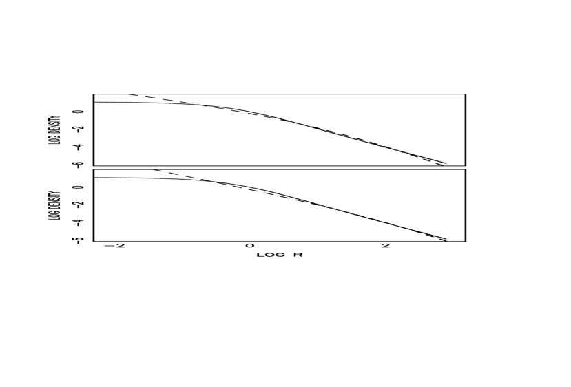
Figure 1: Density of logarithmic potential (solid lines) as function of radius (in units of the core radius $R_{0}$) as compared to those of closest (by inspection) NFW model with central density increasing as $1/R$ (top), and more concentrated systems with density increasing as $1/R^{1.5}$ (bottom).

The main role of the disk component is to introduce strong asymmetry normal to its plane and to reduce it in that plane. Although an exponential disk is most realistic, we have decided to use the Miyamoto-Nagai (1975) model, because in some cases we will be comparing our results with the self-consistent models of Pfenniger (1984b), which had this form for the disk potential. It is also easily handled computationally with the force obtained in closed form by taking the derivatives of the potential given by

$$\Phi_{D}=-\frac{GM_{D}}{\sqrt{x^{2}+y^{2}+\left(a_{d}+\sqrt{b_{d}^{2}+z^{2}}\right)^{2}}},$$ (6)

where $GM_{D}$ is the mass of the disk, in units of $G=1$. The parameters $a_{d}$ and $b_{d}$ determine the central concentration and the flatness of the disks. They are taken to have values of $2.5$ and $0.5$ respectively. The disk mass is always taken to be $GM_{D}=0.2$.

A rapidly rotating bar with a pattern speed $\Omega_{b}$ has been added in the plane containing the halo minor axis. This plane also contains the disk when it is present. The bar model used was a Ferrers ellipsoid of order two (Binney & Tremaine 1987; Pfenniger 1984a). The density of the Ferrers bar is constant along contours given by

$$m^{2}=x^{2}/a_{b}^{2}+y^{2}/b_{b}^{2}+z^{2}/c_{b}^{2},$$ (7)

where $a_{b}>b_{b}>c_{b}$ are the semi-axes of the density distribution. Inside the mass distribution ($m<1$) the density varies as

$$\rho=\rho_{c}(1-m^{2})^{2},$$ (8)

where the central density $\rho_{c}$ is determined by the total mass of the bar $GM_{B}$. The density is zero for $m\geq 1$ .

The bar semi-axes are taken as $a_{b}=6$, $b_{b}=1.5$ and $c_{b}=0.5$, for comparison with Pfenniger’s (1984a,b) main model. The bar pattern speed was always chosen so that the bar extends to corotation — calculated while assuming an axisymmetric halo and not including the bar’s own contribution to the potential. Thus in practice the bar ends inside corotation in accordance with empirical requirement (e.g., Athanassoula 1992). In models where a disk was present, the bar had $20\%$ of the disk mass within the circle tangent to the edge of its major axis.

Models $1-3$ include all the components, the triaxial halo, bar and disk. They are ordered in sequence of increasing halo concentration. Model 1 is a “maximal disk” model while Model 3 is halo dominated at all radii. The rotation curves of these three models are shown in Fig 2. Models $4-6$ are without a disk. This makes it straightforward to quantify the net contribution of the non-rotating non-axisymmetric perturbation — the (constant) equipotential axis ratios measured in the inertial frame in the absence of the bar are simply those of the halo. Model 7 has an axisymmetric halo and a bar only, Model 8 corresponds to main model studied by Pfenniger (1984a) with a bar embedded in a disk without halo. Model 9 deals with triaxial halo only. The complete set of model parameters is given in Table 1.

Figure 2: Rotation curves of Model 1 (top), Model 2(center) and Model 3. Dashed curves represent halo contributions, dashed dotted curves are the disk rotation curves while the solid lines relate to the total rotation curves.

Table 1: Model Parameters

Model	$R_{h0}$	$v_{h0}$	$b_{h}/a_{h}$	$GM_{D}$	$a_{d}$	$b_{d}$	$GM_{B}$	$\Omega_{b}$	Notes
1	10.0	0.2	0.9	0.2	2.5	0.5	0.029	0.031	Triaxial halo with disk, bar
2	2.0	0.2	0.9	0.2	2.5	0.5	0.029	0.041	Triaxial halo with disk, bar
3	0.5	0.2	0.9	0.2	2.5	0.5	0.029	0.042	Triaxial halo with disk, bar
4	0.5	0.2	0.9	–	–	–	0.03	0.033	Triaxial halo, bar w/o disk
5	0.5	0.2	0.95	–	–	–	0.03	0.033	Triaxial halo, bar w/o disk
6	0.5	0.2	0.99	–	–	–	0.03	0.033	Triaxial halo, bar w/o disk
7	0.5	0.2	1.0	–	–	–	0.03	0.033	Axisymm. halo, bar w/o disk
8	—	—	—	1.0	3.0	1.0	0.1	0.052	Pfenniger model (disk, bar)
9	0.5	0.2	0.9	–	–	–	–	–	Triaxial halo only

5 Coordinate system, initial conditions and integrator

We employ the coordinate system of Pfenniger (1984a), whereas the canonical phase space variables are given by (x,y,z,X,Y,Z) and through these the Hamiltonian is defined as

$$H=\frac{1}{2}\left(X^{2}+Y^{2}+Z^{2}\right)+\Phi(x,y,z)-\Omega_{b}\left(xY-yX\right),$$ (9)

where the potential $\Phi$ is given by the sum of the contributions described in the previous section. In this system the spatial coordinates refer to a frame uniformly rotating with the bar with angular velocity $\Omega_{b}$, while the velocities are measured in the inertial frame. The coordinates of the halo, assumed to be non-rotating, are rotated back according to $x_{h}=x\cos(\Omega_{b}t)-y\sin(\Omega_{b}t)$ and $y_{h}=x\sin(\Omega_{b}t)+y\cos(\Omega_{b}t)$. Once calculated, the halo force is then transformed back into the rotating frame in a similar manner.

Our goal is to investigate the stability of candidate trajectories which may support a bar embedded in different disk-halo configurations. For this purpose the following initial conditions are appropriate. We start slightly above the $x$-axis, directed along the bar major axis. The initial amplitude of the $z$-offset is taken as 20 pc for runs, except for those in Section 6.3 where the initial $z$ excursion is increased to 200 pc. The velocities of the particles are taken normal to the $xz$-plane: that is the only nonzero component is $Y$, also taken to be positive. This means that our trajectories are symmetric with respect to the $x$-axis and they are also, at least in the absence of additional triaxial perturbation, prograde. In the case where the halo is axisymmetric, these initial conditions, within the limit of resolution in the initial $x$ and $Y$ values, produce all trajectories parented by the $x_{1}$ periodic orbits aligned with the bar. These are known to be the building blocks of self-consistent bars (e.g., Pfenniger 1984b, where they are termed B orbits).

The binning of the initial conditions is done on a linear equal-spacing grids with 100 subdivisions in each of these coordinates. Thus in total we have, for each model, 10,000 trajectories, with 100 of them starting from each $x$ position. The maximum $x$ position is taken to be the bar major axis (6 kpc) and the maximal $Y$ velocity at each radius is $1.25$ times the local rotation speed assuming an axisymmetric halo (and neglecting the bar’s own contribution).

In some of the figures trajectories will be labeled sequentially in the following manner. The trajectories with the lowest initial $x$ coordinate are taken to be the first hundred. They are ordered in ascending manner according to their value of $Y$. Thus the trajectory having the lowest rotation velocity is number one and that having the highest is number 100. Next come the trajectories with the second lowest initial $x$ values, again ranked in ascending order, according to their initial $Y$ values. And so on in a way that the last hundred (those with rank 9,900 to 10,000) trajectories start with largest initial $x$ values in ascending order in $Y$.

The integration is advanced using the variable order variable stepsize Adams method as implemented in the NAG routine D02CJF with a local (per timestep) tolerance of $10^{-10}$. Even at this low tolerance level there is no guarantee that the chaotic trajectories integrated are the actual trajectories of the system from the given initial conditions. Indeed, varying the tolerance level gave usually different trajectories. This is because the problem is inherently unstable. Nevertheless, it was found that for the range of tolerance $10^{-8}-10^{-14}$, trajectories were qualitatively similar, as evidenced by their occupation numbers on the grid of Section 3, for example. In addition, when canonical conjugate initial conditions were chosen for the tangent space vectors (i.e., vectors pointed towards pairs of position and velocity coordinates $(x,X)$, etc.), the Liapunov exponents came in positive and negative pairs to an accuracy of better than a few parts in $10^{8}$. This is a good measure as to the accuracy of the calculation since it implies that the Poincare’ invariants of all order (e.g., Arnold 1989; Sussman, Wisdom & Mayer 2001) are conserved to high accuracy and the symplectic nature of the Hamiltonian system is thus conserved: despite the fact that the integrator is not symplectic by design, it is effectively so.

Except for Section 6.3, where results are presented for trajectories integrated through a time interval of $10,000~{}{\rm Myr}$, all data relate to trajectories evolved for $50,000~{}{\rm Myr}$. Arguments rationalizing the choice of this particular time interval are given in Section 2.

6 Stability of trajectories and configuration space distribution

In this section we will analyze the stability properties of trajectories and their relationship to trajectories distribution in the configuration space. This will be achieved by calculating the Liapunov exponents and by employing the cylindrical grid described in Section 3. Our goal will be to examine the plausibility of self-consistent equilibria for barred galaxy models with different halo structures — differing from each other in their degree of central concentrations and triaxiality. In addition, we would like to know how tight is the correlation between the trajectories’ distribution in the configuration space and their stability properties.

6.1 Maximal exponent and configuration space volume

6.1.1 The effect of central concentration

To get a measure of the configuration space volume occupied by a given trajectory we calculate the total volume of the cells which it visits. This volume is normalized in terms of the bar’s volume within the trajectory starting point, i.e., the volume of the bar between two planes normal to the major axis of the bar at the starting point (and its reflection). The results for Models $1-3$ are shown on the left-hand panels in Fig. 3, which depict a sequence of increasingly centrally-concentrated halos with core radii decreasing from 10 kpc to 0.5 kpc. The models are presented in the form of grayshade diagrams, with darker shading corresponding to larger relative volume occupied by a trajectory. The positions on the diagrams correspond to the initial conditions — with the vertical axis rescaled in terms of the local rotational speed at the initial $x$ value labeled on the horizontal axis.

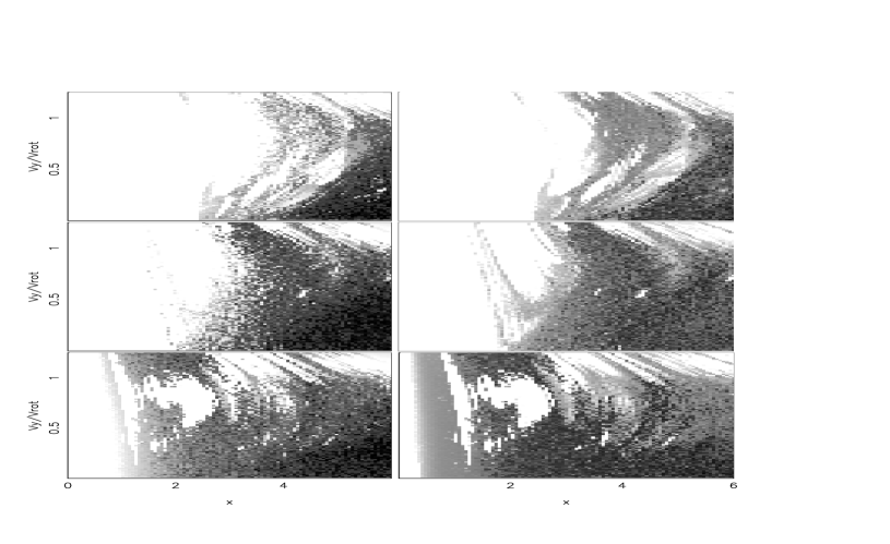
Figure 3: Grayshade diagrams showing configuration space volume (left panels) and maximal Liapunov exponents (right panels) for trajectories of Model 1 (top), Model 2 (middle) and Model 3. The configuration space volume is defined as the total volume of the cells visited by a trajectory and is normalized in units of the volume of the bar within the starting radius of the trajectory. The scale is logarithmic (base ten) with the white background corresponding to values of $-0.5$ and less, and the foreground to values of $2$ (i.e., hundred times the volume of the bar at the initial radius) and more. The exponents are rescaled, so that their inverse is given in units of dynamical time (taken to be the local rotation period in the azimuthally-averaged potential excluding the bar). The scale is logarithmic. The background corresponds to values of $-1.5$ or less (i.e., exponential times of $\sim 32\tau_{D}$ or more and the foreground to values of $0.5$ or more.

The darkest shading corresponds to trajectories occupying a configuration space volume which is 100 or more in the normalized units (see above). Clearly such trajectories (and all those that are represented by the darker spots on this logarithmic scale) cannot contribute towards a self-consistent bar — by virtue of the fact that their spatial distribution is far more extended than the bar at their starting radius. As can be seen, the fraction of such trajectories increases significantly as the halo central concentration is increased: being confined to the outer regions (where the equidensity profiles of the model are themselves more round) in Model 1, but occupying the vast majority of all initial conditions in Model 3. As we will see shortly, these trajectories are chaotic, with large Liapunov exponents. And even though the volume of configuration space occupied by some of the chaotic trajectories in this model is sometimes smaller than corresponding trajectories in the case of $R_{h0}=2$, trajectories with volume significantly larger than the bar are much more abundant. Indeed, in this latter case, except for the “island” around $V_{y}/V_{rot}=0.75$ between initial condition with $1.5$ kpc and $3$ kpc and the very inner region (where the halo potential is nearly harmonic) there are hardly any regular trajectories that are elongated with the bar Moreover, many of the regular trajectories do not match the bar density distribution, being too round by comparison. This is the case of the regular regions corresponding to initial velocities $V_{y}/V_{rot}\gtrsim 0.8$ and initial radii greater than 3 kpc. For as can be seen from Fig. 4, where we plot the distribution of the minimum (cylindrical) radius visited by these trajectories, the majority of trajectories started beyond $x=3$ have minimal radii that are greater than the bars minor axis; they envelop the bar and thus cannot contribute towards building a self-consistent model. Note that the trajectories which do have minimal radii smaller than $1.5$ correspond to the isolated islands of stability corresponding to initial velocities $V_{y}/V_{rot}\lesssim 0.8$. One can, therefore, conclude that the sequence of Models $1-3$ represents progressively more unstable bars which will tend to evolve quickly, since the system does not support the kind of trajectories required to build such a bar self-consistently.

Figure 4: Distribution of minimal radii of regular trajectories (defined here as those having configuration volume smaller than the bar’s at their starting radius) of Model 3 with initial coordinate $x\geq 3$.

From the right hand-side panels of Fig. 3 one observes that most of the trajectories occupying large regions of the configuration space are chaotic. Furthermore, comparison of left and right panels shows that there is quite a tight correlation between the values of the Liapunov exponents and the volume of configuration space the trajectories move in. This, of course, should not come as a surprise. For as explained in the introduction and in Section 2, regular orbits are confined by invariants which characterize the regular motion while chaotic ones are under no such constraints. Trajectories with higher Liapunov exponents, in addition to having smaller instability timescales, are also typically found in regions of phase space away from regular trajectories and barriers, such as cantori which can prevent phase space transport (e.g., Wiggins 1991). This implies that, in a given time, they are to diffuse in larger regions of phase space, which is then reflected in their configurations space distribution. Nevertheless, the degree of correlation is stark and shows the intimate relation the question of stability of trajectories bears to that of self-consistency of galactic models.

There are two effects which may be leading to the increase in the fraction of chaotic trajectories with the decrease in the halo core radius. The first, as discussed in the introduction, is the increased nonlinearity introduced by the centrally-concentrated mass distribution — which leads to increased coupling between the degrees of freedom. The second is the increased time dependency in the force field. For, as can be seen from Fig. 5, where we plot the ratios of the non-integrable components of the bar and halo force fields, for the least centrally-concentrated halo ($R_{h0}=10$) it is only at the edge of the bar that the average azimuthal force component of the halo becomes comparable to that of the bar. In the case of $R_{h0}=0.5$, on the other hand, this component is of the order of the corresponding bar component at all radii. For mild halo triaxialities, therefore, it is necessary that the halo be centrally-concentrated for the effect of time dependency to become important.

Figure 5: Ratio of the average of the absolute value of the bar’s azimuthal force to that of the halo, for halo axis ratio $b/a=0.9$ and for different core radii. The bar’s relative contribution is seen to be strongest when the halo has a large core radius $R_{0}=10$, weakest for a centrally-concentrated halo $R_{0}=0.5$ and intermediate for $R_{0}=2$.

6.1.2 The effect of halo triaxiality

We now attempt to look in more detail into the origin of the widespread chaotic behavior observed in the orbital structure of barred systems with centrally-concentrated halo. To more easily identify the strength of the non-rotating non-axisymmetric contribution to the potential, we now remove the axisymmetric disk from our superposition of potentials. Removing the disk contribution will obviously increase the effective non-axisymmetric perturbation in the potential. This is expected to increase the region of instability even further. It is apparent, however, that the dominant element producing unstable trajectories near the short axis plane of centrally-concentrated halos in our models is not their own triaxiality but the presence of a rotating barred component. This can be seen from Fig. 6, where we show the grayshade diagrams for a centrally-concentrated triaxial halo with $b_{h}/a_{h}=0.9$, $c_{h}/a_{h}=0.8$. In the absence of the bar, trajectories are regular and are confined in configuration space (Model 9, top panels). The addition of the rotating perturbation, however, modifies the situation dramatically (Model 4, center). For comparison, we show the grayshade diagrams of the model self-consistently constructed by Pfenniger (1984b: Model 8). It is evident that the orbital structure, as manifested by the configuration space distribution and Liapunov numbers, of this model is different from that of models where a centrally-concentrated triaxial halo is present. This of course confirms our original inference that a self-consistent barred system is impossible to sustain inside a triaxial and centrally-concentrated halo: the trajectories it supports are too chaotic and occupy too large a volume of the configuration space to represent a bar.

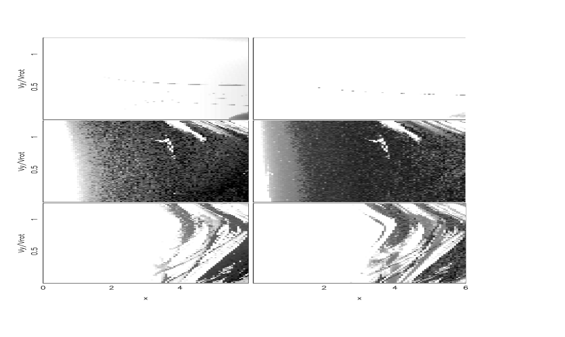
Figure 6: Same as in Fig. 3 but for trajectories of Model 9 (top), Model 4 (middle) and Model 8.

In fact, as will be seen from Fig. 7 (Model 6, middle panels), even very small departures from axisymmetry on the part of the halo (as small as $1\%$ in the potential axis ratio $b_{h}/a_{h}$) can lead to large connected regions of initial conditions corresponding to chaotic trajectories, with only islands of stability in their midst. Only in the limit of a perfectly axisymmetric halo models is it possible to obtain connected regions of regular trajectories at most radii. In that case (bottom panels), significant fraction of the initial conditions are occupied by trajectories that support the bar — the white regions that appear for most initial $x$ up to about 4 kpc represent trajectories that are mostly parented by stable periodic $x_{1}$ orbits, and are thus aligned with the bar. The existence of these trajectories is necessary for the construction of barred equilibria. It is consistent with numerical simulations where long lived bars embedded in centrally-concentrated axisymmetric halos are observed (Ideta & Hozumi 2000; Debattista & Sellwood 2000; Athanassoula & Misiriotis 2002). These may slowdown in time but do not dissolve. In some of these simulations rings surrounding the bars are also found. These are possibly related to the trajectories represented by the white strips on the upper right corner of the diagrams in the bottom panels of Fig. 7. These regions correspond to nearly round trajectories which, at the outer edge of the bar and slightly beyond, are elongated in the direction perpendicular to the bar — as is observed in the simulations.

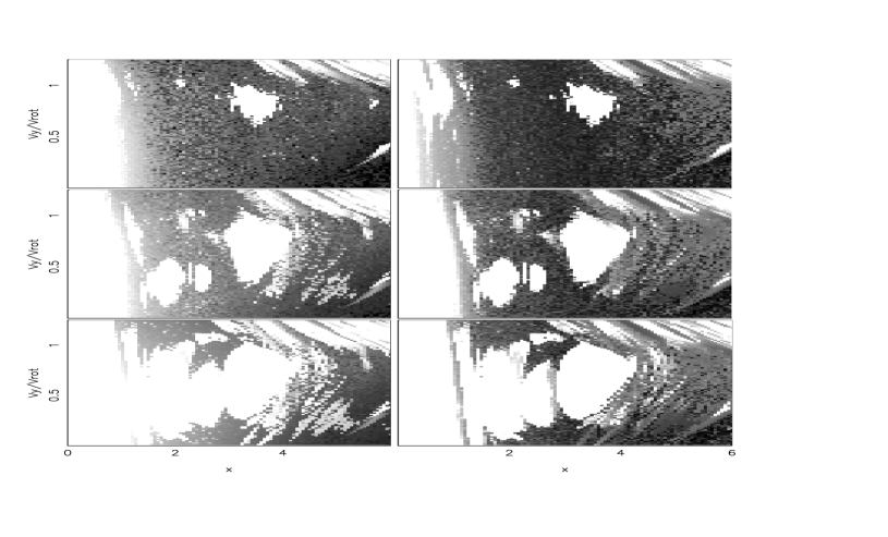
Figure 7: Same as in Fig. 3 but for trajectories of Model 5 (top), Model 6 (middle) and Model 7.

The fraction of bar supporting regular trajectories decreases rapidly as small non-axisymmetric perturbations are applied. In the case of Model 6 orbits elongated along the bar still exist at most radii. However they occupy a much smaller fraction of the initial conditions than in Model 7. The range of shapes they come in is therefore narrower, which implies that it is less probable that among them will be found those that match the bar’s asymmetry (i.e., are not too fat). Indeed, we find by inspection that a large fraction of the available trajectories that are elongated along the bar do not match its asymmetry. Further departures from axisymmetry render the bar supporting orbits exceedingly rare. In Model 5 (Fig. 7, top panels) they are found at a small starting range in $x$. In model 4, they are virtually non-existent.

The above implies that our axisymmetric model is structurally unstable — since any small perturbation renders the once connected regular regions into disjoint sets. The replacement of regular trajectories parented by the $x_{1}$ orbits by chaotic ones in turn implies that self-consistent bars are unlikely under these circumstances. Because the perturbations required are very small, axisymmetric models of barred galaxies with centrally-concentrated halos must then be considered non-generic.

6.2 Vertical stability of trajectories

The conclusion that systems with centrally-concentrated triaxial halos are unlikely supporters of bars is impressed further when one looks at the vertical stability of the trajectories under consideration. In Fig. 8 we show, for some of our models, grayshade diagrams representing the fraction of time trajectories spend in cells that correspond to vertical excursions greater than the semi-minor of the bar. It is evident that for models with even minor triaxiality this fraction can exceed one-half of the time for a large number of trajectories. Note that this is necessarily an underestimate — the bar’s extension is, except at the origin, always less than the minor axis value.

Comparison of the structure of the grayshade diagrams in Fig. 8 with those in Fig. 6 and Fig. 7 reveals that the fraction of time a trajectory spends having large absolute values for its vertical coordinate correlates well with the values of the Liapunov exponents. In other words, trajectories which spend the largest fraction of time at large $z$ have largest Liapunov exponents. This in turn correlated with the total configuration volume they occupy. Thus vertical stability is a simple diagnostic of chaotic behavior: almost all regular trajectories conserve their initially small amplitudes of $z$ oscillations (the exceptions are those near bifurcations leading to three dimensional regular orbits). It is also a sufficient criterion that orbit densities do not match that of the bar, being too extended in the vertical direction.

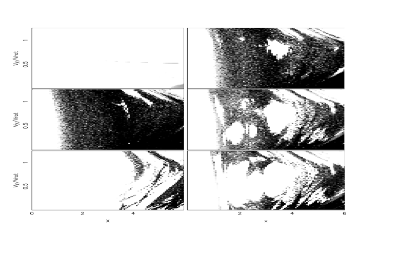
Figure 8: Grayshade diagrams showing the fraction of time trajectories spend at cells comprising vertical coordinates larger than the bar minor axis. Left panel: Model 9 (top), Model 4 (middle) and Model 8 (as in panels of Fig 6). Right panel: Model 5 (top), Model 6 (middle) and Model 7 (as in panels of Fig 7). The shades are on a linear scale whereas the foreground corresponds to trajectories spending $75\%$ of their time or longer in the aforementioned cells and the background corresponds to trajectories spending $0.075\%$ of the integration time in such cells.

We find that the maximal vertical excursion of chaotic trajectories of some of our models can be quite large — of the order of 10 kpc. To illustrate this, we have arranged the trajectories in ascending order according to their starting spatial and velocity coordinates (see Section 2) and plotted the logarithm of their maximal vertical excursion within the first $10,000$ Myr. The results are shown in Fig. 9.

6.3 Evolution on shorter timescale and the instability in- and out-of-the plane

Some trajectories which have large Liapunov exponents, and according to the diagrams of Fig. 8 spend a large fraction of their time at $z$ coordinates larger than the bar’s vertical extension, nevertheless appear to have small maximal vertical excursion in Fig. 9. This happens because many of these trajectories do not, for the small initial $z$ amplitude we used, reach their maximal $z$ extension in $10,000$ Myr. We had chosen the small initial $z$ amplitudes in order to detect trajectories that may be vertically unstable even if their maximal excursions do not exceed a few hundred pc. In realistic situations however, vertical motions would be sufficient so that stars already have $z$ amplitudes of such magnitude.

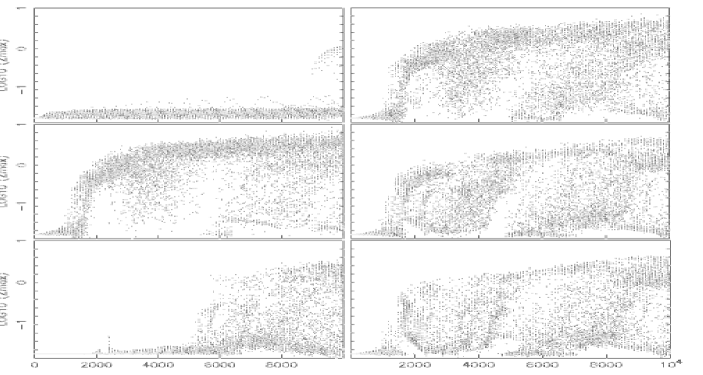
Figure 9: Maximal vertical excursion within $10,000$ Myr. The panels correspond to those of models shown in Fig. 8. The trajectories are arranged in ascending order such that those at smaller initial radii have strictly smaller number than those starting at a larger radius. At each radius the rank progressively increases with initial normal velocity (cf., Section 5).

We have rerun some models with the larger initial $z$ amplitude of $0.2$. The results, for Models 4, 5 and 6 are shown in Fig. 10. One finds that many trajectories, that apparently were stable in the $z$ direction over the Hubble time, are now unstable. Fig. 10 (right panels) also displays diagrams, similar to those in Fig. 8, representing the fraction of time trajectories spend in cells comprising vertical coordinates larger than that of the bar vertical extension. This fraction of time now has increased significantly by starting our trajectories at a larger $z$ coordinate value, albeit one that still is significantly smaller than the bar’s semi-minor axis. This suggests that the vertical instability is important in determining the orbital properties of the system, transforming trajectories that are stable in the plane into unstable ones, but that it manifests itself over relatively long time-scale, especially when the initial perturbation is small.

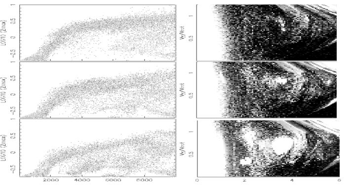
Figure 10: Maximum vertical excursions (left panels) and grayshade diagrams showing the time fraction spent at configuration space cells comprising vertical coordinates larger than the bar minor axis for Model 4 (top), Model 5 (middle) and Model 6 (with the same scaling as in Fig. 8. Trajectories are integrated for $10,000$ Myr starting with a vertical amplitude of $0.2$ kpc (instead of the canonical $0.02$ kpc used in the other runs).

Trajectories having large vertical extensions and spending most of their time with absolute values of their $z$ coordinates larger than the bar’s semi-minor axis cannot contribute towards a self consistent barred galaxy model. This being the case for most trajectories of Models 4,5 and 6, makes it apparent that the bar would not survive in such models for a Hubble time — which places an upper limit on the dissolution time of any barred system embedded in mildly triaxial centrally concentrated halo. A lower limit, which should be of the order of the Liapunov timescale of the chaotic trajectories, is of the order of a few dynamical times. This should be the time-scale for bar dissolution in the most chaotic systems (e.g., Model 4) where hardly any regular trajectories exist. In such cases, the vertical instability is unlikely to be of central importance in the evolution of the system — since the bar would probably dissolve in the plane before its presence becomes felt.

Fig. 11 shows the maximal Liapunov exponents and the configuration space volume for Models 5, 6 and 7 for trajectories integrated through this smaller period of time and starting with larger $z$ amplitude (note the difference in grayscales of Liapunov exponents). Again one observes a clear similarity between the distribution of values of the exponents and the occupied configuration space volume. The figures are qualitatively similar to the ones integrated for $50,000$ Myr from $z_{in}=0.02$ (cf. Fig. 7). Quantitatively there are some differences. The extent of the shaded regions has increased. Unstable trajectories are now more abundant. This is again an effect of the larger initial vertical amplitudes used here, causing chaotic trajectories to replace regular ones. However the most unstable trajectories now have somewhat smaller configuration space volume than previously. This suggests that trajectories continue to explore new regions of phase space as the system evolves in time. It is not surprising, given the time-dependent nature of the potential (meaning an orbits phase available space is not necessarily bounded) and the possibility of the presence of “sticky” chaotic trajectories that take long times to achieve an invariant distribution even for the time-independent case (e.g., Siopis & Kandrup 2002).

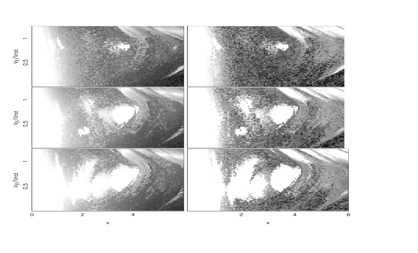
Figure 11: Same as in Fig. 7 but for trajectories integrated for $10,000$ Myr and with initial vertical condition $z=0.2$ kpc (instead of the canonical $0.02$ kpc used in the runs in that figure). Note that, to adjust for the significantly shorter integration time, which implies that regular trajectories would have an exponent that is proportionally larger, the background for the grayshades representing these quantities is rescaled to -0.9 (instead of -1.5 as in Fig. 7).

Indeed simple inspection of the spatial distribution of trajectories showed that both these effects are at work; some trajectories keep on moving towards larger and larger radii and vertical excursions, while others stay within a bounded region but fill larger and larger volumes within that region. In the latter case this mainly consisted of trajectories with a hollow configuration space distribution, which was being filled up as the integration proceeds. There are also some trajectories whose vertical extension is only significant after 10 Gyr. None of the trajectories examined however had a spatial configuration that did not match the bar over 50 Gyr but did match the bar over $10$ Gyr. In fact, the vast majority already showed a spatial structure in the plane which is very different from that of the bar within 500 Myr or so — their shapes being too isotropic, even though they were launched from initial conditions corresponding to thin bar-aligned orbits in the case when the halo is axisymmetric. Vertical instability generally took longer to develop, but was far faster, as expected, when the initial vertical perturbation was larger.

Furthermore, trajectories that occupied a relatively (compared to the bar) large configuration space over the longer times integration still do over the span of $10$ Gyr. This can be seen from Fig. 12 where we plot the relative volumes of the trajectories of Model 6 for the two cases against the volumes of the case where the trajectories are integrated for $50$ Gyr. As expected, trajectories which, for the case of long integration from small initial $z$, had small phase space volumes usually acquire a much larger one. This is due to the enhanced $z$ instability which further destroys the regular regions. On the other hand, trajectories which had large configuration space volumes compared to that of the bar and had pronounced $z$ excursion, even when starting from $z=0.02$, now have smaller volume. Nevertheless, this is still much larger than the that of the bar — again confirming that they are unlikely to contribute towards a self-consistent model on the timescale of $10,000$ Myr.

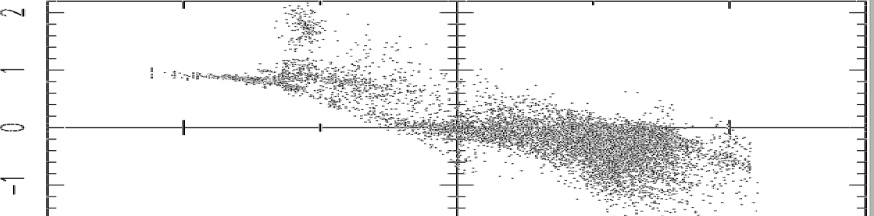
Figure 12: Comparison of the configuration space volume for trajectories integrated for $10000$ Myr (and stating AT $z=0.2$) and ones integrated for $50000$ Myr (and starting at $z=0.02$). The the horizontal axis represent values of the (base ten) logarithm of the configuration space volume of the latter trajectories, while the vertical axis represents logarithms (again base ten) of the ratio of the two volumes for the different trajectories of Model 5 (i.e., $vol(10000,i)/vol(50000,i),i=1,10000$).

6.4 Full set of Liapunov exponents and distribution of exponential times

Because it is CPU-time consuming to calculate the full set of Liapunov exponents at high resolution in the initial conditions, we performed this task for a selected set of models. The values of these exponents provide information on whether trajectories, though being chaotic, may conserve (even if approximately) some quantities with time. Fig. 13 shows grayshade diagrams involving the second and third Liapunov exponents of trajectories in the three models, 5, 6 and 7, whose configuration space volume and maximal exponents are shown in Fig. 7. The agreement between the configuration volume of trajectories and the values of their exponents is even more precise than in the case of the maximal exponent — most discrepancies, even though minor originally, having now disappeared. The additional constraints provided by low values in the two smaller Liapunov exponents account for the remaining regions of initial conditions corresponding to small configuration space volume despite having large values of the maximal exponent.

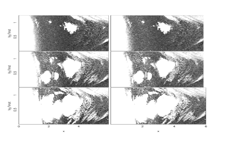
Figure 13: Grayshade diagrams for the middle (left panels) and smallest Liapunov exponents for Model 5 (top), Model 6 (middle) and Model 7. On the (base ten) logarithmic scale the middle exponent background value is $-1.5$ and foreground is $0.2$ while for the smallest exponent the background is scaled to $-2$ and foreground to $0$.

The sum of the positive exponents for a given trajectory characterizes its Kolmogorov entropy (see Appendix). For a group of nearby trajectories in connected phase space region it measures the rate of increase of the coarse-grained volume they occupy, and thus of the evolution of their statistical distribution. The inverse of this entropy (strictly speaking multiplied by a numerical factor of order unity that is ignored here) defines a timescale for such evolution.

In Fig. 14 we display histograms showing the distribution of the inverse of the Kolmogorov entropy for trajectories of Models 7, 6, 5 and 4. As can be seen, for trajectories of axisymmetric Model 7, the corresponding exponential times are mostly very large, of the order of the Hubble time. These correspond mainly to trajectories trapped around the $x_{1}$ periodic orbit family aligned with the bar (the large connected white patch in the grayshade diagrams in the bottom panel of Fig. 7). Moreover, the more unstable trajectories, with smaller exponential timescales, are of roughly equal numbers over a large range of values; the distribution is relatively flat, being only slightly bimodal on far left of the figure. These are exponents of various higher order regular or trapped chaotic trajectories — i.e., ones existing in regions of phase space where mainly regular orbits dominate. The final peak corresponds to trajectories starting from initial conditions in the outer region of the system (cf., Fig. 7 bottom panel), which correspond to regions of phase space that are dominated by chaotic trajectories.

Figure 14: Histograms showing the distribution of the exponentiation times (taken to be the inverse of the Kolmogorov-Sinai entropy) for trajectories of (from top to bottom) models 7, 6, 5 and 4.

As the non-axisymmetric perturbation is increased, regular trajectories aligned with the bar progressively become less abundant. Initially there is an equal increase in the number of trapped trajectories (second peak on left for histogram of Model 6) and highly chaotic ones (first peak). Eventually, however, the increase in the latter occurs at the expense of the former (Model 5). Finally, the fraction of both the trapped and regular trajectories becomes very small (Model 4). Here most trajectories are highly chaotic, part of the same connected “stochastic sea,” with exponentiation timescale varying relatively little. This is expected since, for Model 4 (cf. Fig. 6, middle panel), except for small regular regions, trajectories form a connected region of initial conditions that have similar Liapunov exponents and configuration space volumes.

For Model 4, most of the remaining regular trajectories are parented by surviving higher order periodic orbit families of the resonant zones (the white strips in Fig. 6 middle panels). None are parented by the $x_{1}$ family of the unperturbed axisymmetric halo case. Almost certainly, the absence of a significant fraction of regular orbits, more importantly the total absence of any regular orbits aligned with the bar, ensures that such a bar cannot be built self-consistently. For in the case of a time-independent potential, for example, any set of initial conditions starting in a connected chaotic region will evolve to an invariant distribution, with every trajectory having the same time-averaged phase space distribution in as all other trajectories. The projection onto configuration space of such a distribution would be too isotropic to match a bar. In the case of a time-dependent system, the region in which trajectories move is not necessarily bounded by a zero velocity curve, and therefore some trajectories can explore even larger volumes as their energies change — an effect that is likely to make the discrepancy more pronounced.

7 Energy decorrelation

For trajectories with large maximal exponent, the other two positive exponents are proportional to it with a nearly constant of proportionality. This is not always true, however, of trajectories with smaller maximal exponent. The latter tend to have relatively even smaller corresponding values for the two smaller exponents. This is illustrated in Fig 15 where we plot the Liapunov exponents of trajectories of Model 4. It is especially clear for trajectories starting in the inner regions (those with small trajectory numbers). It turns out that such trajectories also conserve their energy well.

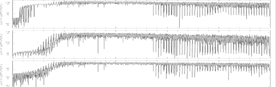
Figure 15: Liapunov exponents of Model 5 for trajectories arranged sequentially such that the first hundred correspond to initial conditions at the first position bin and progressively larger normal velocities (cf., Section 5).

Energy, always an invariant quantity in a time-independent potential, is allowed to vary in the time-dependent models described here. Corresponding to energy conservation is a pair of zero Liapunov exponents. Therefore, trajectories that conserve energy well will have at least one small exponent. In order to test energy (i.e., the Hamiltonian of Eq. [9]) conservation, we calculated the correlator $C_{i}=\frac{<E(t)E(t+\tau i)>}{<E(t)><E(t+\tau)>}$, where $\tau$ is a time interval, taken as 500 Myr, and $i$ is an integer. The quantity $C_{i}$ as defined above is zero if there is complete loss of memory in energy over a timescale $\tau i$, and one if there is no loss whatsoever, — for example, if energy is conserved along a trajectory. It can also be seen as an angle between a normalized unit vector, consisting of the values of the energy at intervals $\tau i$, and another “delayed” vector with corresponding points delayed from the first vector also by an interval $\tau i$.

In Fig. 16 we plot $\log_{10}(1-C_{i})$ for $i=1,10$, as well as the relative dispersion in energy along our enumerated trajectories of Model 4. As expected, in the region where two of the Liapunov exponents have very small values, energy correlation is large (that is near 1) and the dispersion is small. What is somewhat surprising is that, for larger radii, the energies of the trajectories at different times appear to be again correlated — this despite the fact that these trajectories belong to large connected regions with high values of the exponents (cf. Section 6.1.2).

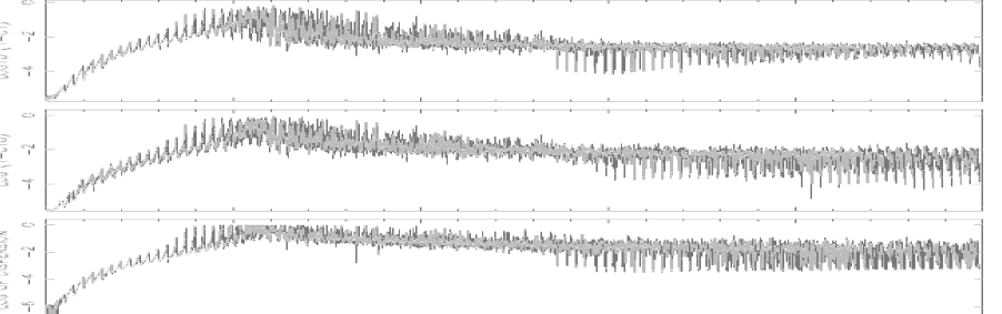
Figure 16: Energy correlators $C_{i}=1-\frac{<E(t)E(t+\tau i)>}{<E(t)><E(t+\tau)>}$ averaged over $50,000$ Myr with interval $\tau i$ and $\tau=500$ MYr (Top: $i=1$, Middle: $i=10$), and relative energy dispersions (bottom) for Model 5. Trajectories are arranged sequentially such that the first hundred correspond to initial conditions at the first position bin and progressively larger normal velocities (cf., Section 5).

The variation of the dispersion and the quantities $\log_{10}(1-C_{i})$ as a function of radius appear to follow closely the strength of the bar perturbation (Fig. 17). This trend does not seem to be substantially altered by changing the asymmetry of the halo (we have checked this by comparing the results presented here with analogous ones for Models 5 and 6). Thus, for any non-axisymmetric perturbation between one and ten percent in the nonrotating potential, energy conservation of trajectories starting at radii where the bar asymmetry is maximal is affected considerably. For other trajectories, energy conservation is not significantly affected by such small perturbations. One can perhaps say that the value of their Hamiltonian is stable along their trajectories.

Figure 17: Average (of absolute value of) azimuthal bar force as a function of radius.

It is interesting that a time-dependent perturbation can have such a large effect on the stability properties of some trajectories and the manner in which their configuration space distribution behaves, but causes very little change in energy. It illustrates the fragility of orbital structure of the unperturbed axisymmetric system.

8 Conclusions

In this paper we have analyzed the stability and configuration space properties of trajectories starting near the plane containing a bar in galaxies with different dark matter halo distributions. In particular, we examine the variation of these properties for different concentrations (Section 6.1.1) and triaxialities (Section 6.1.2). This is done by calculating the Liapunov exponents, looking at the time-averaged spatial density distribution (Section 6) and the vertical stability properties (Sections 6.2) of samples of $10,000$ trajectories starting near the plane containing the bar in each model. As a reference we have compared these properties with those of the relatively stable model that has been built self-consistently by Pfenniger (1984a,b). For some of the models we also calculate the full set of Liapunov exponents and look at the distribution of exponential timescales inferred from the Kolmogorov entropy (Section 6.4). In general, there is remarkable correlation between the local stability properties, as characterized by the exponents, and the the spatial distribution of trajectories, as quantified, for example, by the configuration space volume they fill — with the more unstable trajectories occupying much larger volume than more chaotic ones.

For models with centrally-concentrated halos, we find a large fraction of trajectories to be chaotic. These fill a large (compared to the bar’s) volume of the configuration space and spend most of the time at vertical extension greater than the maximum thickness of the bar. They are, therefore, unlikely to contribute towards a self-consistent model. In addition many of the trajectories that remain regular have minimum extensions in the plane larger than the bar’s middle axis. They also cannot contribute towards a self-consistent model (Section 6.1.1).

The above is even true to some extent in the case when the halo is centrally-concentrated but axisymmetric. Still, in this case, there remains large connected sets of initial conditions corresponding to regular orbits which are aligned with the bar and could contribute to a self-consistent model. When, however, the halo is triaxial, chaotic trajectories become a dominant majority — even very small halo triaxiality (a $1\%$ perturbation in the potential axis ratio) causes the chaotic regions to become connected and regular phase space regions to become islands of stability (Section 6.1.2). Such models are unlikely candidates for steady state self-consistent solutions.

There are several reasons why centrally-concentrated halos, especially triaxial ones, contribute to the chaotic behavior displayed from most initial conditions. A centrally-concentrated mass distribution has solutions for the Poisson equation that is far from quadratic, in the sense that an expansion of the potential power series has large terms beyond the quadratic. This produces a coupling between different degrees of freedom in equations of motions which are highly nonlinear. In the axisymmetric halo case these systems generically have no global integrals of motion other than energy (in the rotating frame) and, being far from linear, are, therefore, candidates for supporting large (phase space) regions of chaotic trajectories. When a nonrotating triaxial halo is added even energy is lost as an integral of motion. Since time translation symmetry is broken, such a system has no obvious symmetries and is likely to exhibit chaotic behavior from most initial conditions, as indeed is found to be the case. Moreover, in the case of a halo with a significant core, and for mild triaxiality, the non-axisymmetric halo perturbation is completely negligible in the bar region. This is another reason why central concentration triggers chaos; for centrally-concentrated halos of mild triaxiality the bar and halo azimuthal forces in the equatorial plane become comparable. There are no frames of reference where the system may be considered, to some approximation, stationary.

It is significant that very small deviations from axisymmetry in the halo potential can produce drastic changes in phase space structure. Systems where neither KAM stability (a property of separable systems: see, e.g., Arnold in Mackay & Meiss 1987) guarantees that small perturbations do not drastically change phase space structure or where structural stability (a property of strongly chaotic systems, e.g., C systems: Anosov 1969) ensures the robustness of qualitative properties of trajectories, are candidates for such behavior. In other words, systems with a mixed phase space, where regular and chaotic trajectories coexist, are always liable for strong modification of qualitative properties by means of small perturbations. This appears to be the case for models of centrally-concentrated barred galaxies with axisymmetric halos. A small perturbation in the halo axis ratio can, as we have seen, have a significant effect (cf., Fig 7). These systems are said to be structurally unstable. Modeling barred galaxies with centrally concentrated halos while assuming that these halos are axisymmetric may, therefore, produce non-generic results.

Even though we find some correlation between the energy change of trajectories of triaxial systems and the values of Liapunov exponents, many trajectories that are unstable over a dynamical time conserve energy quite well (Section 7). This was inferred by calculating the energy correlation over times up to $5$ Gyr and the dispersion in its values averaged over $50$ Gyr. We find that only for a small fraction of the chaotic trajectories does energy decorrelate over this period and the dispersion in its values becomes large. This shows that long timescales for energy relaxation do not imply that evolution of other quantities does not happen at a much larger rate, as is the case with the $z$ instability, for example.

Halos identified in cosmological simulations with CDM initial conditions are found to be both centrally-concentrated and triaxial. The results presented in this paper, therefore, suggest that the existence of such structures around galaxies containing strong large-scale bars is probably ruled out. Furthermore, the very small departures required from axisymmetry suggest that our results are generic — in the sense that departures from perfect axisymmetry, due to halo substructure, for example (another prediction of CDM models), may be sufficient for the effects found in this work to become important. These findings can, therefore, be considered consistent with the growing observational evidence against such halos in present day galaxies.

It has been suggested that primordial bars in centrally-concentrated halos can act as to reduce the central concentration of the halo (e.g., Binney, Gerhard & Silk 2000; Weinberg and Katz 2001). If anything, the large fraction of chaotic trajectories found here and the torques resulting from the interaction of two non-axisymmetric structures would enhance such coupling — and that would include the effect of bar breaking investigated by Debattista & Sellwood (2000).

This, however, raises an important question as to whether bars would form in the first place, or survive long enough, in unmodified CDM halos to produce these effects. Athanassoula & Misiriotis (2002) found that not only bars can form in centrally-concentrated, but axisymmetric, halos, but that they are actually much more pronounced that ones in less concentrated halos. The results presented here suggest that small non-axisymmetric perturbations may act as to destroy these bars. Indeed, we find strong vertical instabilities at the outer parts of our axisymmetric model with centrally-concentrated halo (Model 7) which could explain the “X” structure of modeled bars when seen edge on. These vertical instabilities move inwards and become more pronounced when a non-axisymmetric perturbation is present.

The vertical orbital instability observed was found to proceed in tandem with the orbital dissolution in the $xy$-plane. If the latter is rapid, the vertical instability will saturate and is not likely to play an important role — since it almost invariably takes longer time to develop than the instability in the plane. This is especially true if the initial distribution is very thin, in which case the vertical instability timescale can be very long compared to the one in the plane. This is probably the reason why Ideta & Hozumi (2000) concluded that the vertical instability of an $N$-body bar immersed in a centrally-concentrated halo does not make an essential contribution to its evolution. We find that, in this case, the trajectories would quickly mix in the $xy$-plane, evolving towards a spatial distribution which is isotropic there and forming a lens-type configuration. On the other hand, if there is sufficient time for the vertical instability of trajectories to develop, it can play a central role in the evolution. For it is especially in the intermediate cases where the instability in the plane may not be sufficient in dissolving the bar over short timescales that the additional vertical instability may be essential (Section 6.3). The final shape of the dissolved object may then be closer in appearance to a spheroidal component.

If collective instability, leading to bar formation, is active in the case of centrally-concentrated triaxial halos, a bar-like structure may appear. But if the evolution time of the density distribution away from the barred configuration is simply related to the Liapunov timescale of the chaotic trajectories filling the phase space, such a configuration will have to be washed out in a few dynamical times. This should almost certainly be the situation in systems where the non-axisymmetric non-rotating perturbation reaches $10\%$. In this case there are no regular trajectories supporting the bar. Most initial conditions lie in what appears to be a connected chaotic region of phase space composed of unstable trajectories with e-folding time of the order of $10^{8}$ Myr or smaller (cf., Fig 14, bottom panel). It is also probably the case for systems with a perturbation of $5\%$ (Fig. 14, second panel from bottom). Can the presence of a centrally-concentrated triaxial halos in the initial stages of galaxy evolution be the cause of apparent decrease in the bar fraction at redshifts greater than 0.5 (e.g., Abraham et al. 1999)?

In the case of the “mixed” phase space of systems with with smaller non-rotating perturbations the situation is more ambiguous. Nevertheless, even a system where the non-rotating component has a potential axis ratio as large as $0.99$ displays large connected regions of initial conditions leading to strongly chaotic trajectories. A comparison between the bottom panel of Fig. 6 and middle panel of Fig. 7 reveals that the configuration space structure and orbital stability properties of such a model is significantly different from that of the model successfully built in a self-consistent manner by Pfenniger (1984a,b) — with the latter containing far more regular trajectories occupying a small configuration space volume aligned with the bar. In particular, while both models contain, at most radii, orbits that are aligned with the bar, the variety of available such trajectories is far larger in Pfenniger’s model. Indeed, simple inspection of the spatial structure of a sample of bar aligned orbits of Model 6 showed that a large fraction of these are too round to contribute towards a self consistent model.

The preponderance of chaotic trajectories occupying large configuration space volumes, and the apparent absence of a sufficient population of regular bar-supporting orbits, suggest that even models with slowly rotating non-axisymmetric perturbations of $\sim 1\%$ cannot have time-independent equilibria. The question arises as to whether the resulting time dependence would take place on a physically relevant timescale. This is not a trivial question, since in systems with such mixed phase space diffusion times of chaotic trajectories can sometimes be very long. However, in the cases studied here, unless the isolated regions of regular orbits aligned with the bar constitute a sufficient contribution towards a self consistent model, the bar would have to dissolve in a timescale significantly smaller than a Hubble time. Since we know from Section 6.3 that for mildly triaxial centrally-concentrated halos the configuration space volume of most trajectories is also far larger than the bar’s over this period.

It is possible, on the other hand, that central cusps in dark halos have been destroyed during the formation of the baryonic component via processes involving dynamical friction in inhomogeneous baryon background (El-Zant, Shlosman & Hoffman 2001; El-Zant et al. 2002) — or that some fundamental physical process relating to the nature of the dark matter prevents the formation of central density cusps.

Appendix A Evaluation of the Liapunov exponents

A.1 Obtaining the maximal exponent

Even though Liapunov exponents are a widely known classical tool in nonlinear dynamics, only a few studies have used them to quantify chaotic behavior in realistic galactic systems (e.g., Udry & Pfenniger 1998; Merritt & Fridman 1996; Siopis & Kandrup 2000). There is also the recent study by Fux (2001) on the stability of trajectories in a detailed model of the Galaxy. None give a self-contained description of how they are obtained. We, therefore, provide such a description here, since these tools are central to the results in this paper and in the hope that they would find a wider use in the field.

Let a system be described by the first order equations of motion (Newtonian second order equations can be replaced by two first order ones)

$${\bf\dot{X}=F(\bf X},t)$$ (A1)

and their variational (linearised) counterparts

$${\bf\dot{\mbox{\boldmath$\xi$}}=\delta F}.$$ (A2)

Along a particular trajectory ${\bf\bar{X}=\bar{X}}(t,t_{o},{\bf\bar{X}_{o}})$ against which we would like to measure the deviation, with ${\bf X_{o}}$ the initial conditions, (A2) can be rewritten as

$$\dot{\mbox{\boldmath$\xi$}}={\bf D_{x}F(\bar{X}}(t,t_{o},{\bf X_{o}})),\mbox{\boldmath$\xi$}$$ (A3)

where ${\bf D_{x}F}$ is the Jacobian $6N\times 6N$ matrix   ${\bf\partial F_{i}/\partial x_{j}}$   and $i,j=1,6N$. Now let

$${\bf X_{s}=X_{s}(\bar{X}}(t,t_{o},{\bf X_{o}}))$$ (A4)

be the fundamental solution of this matrix with the initial condition being the identity matrix. The solution of (A3) is then given by (Wiggins 1991)

$$\mbox{\boldmath$\xi$}={\bf X_{s}}(t)\mbox{\boldmath$\xi_{0}$},$$ (A5)

which describes the evolution under the linearised dynamics with initial conditions $\xi_{0}$ in the space of linear variations.

A Liapunov exponent is the infinite limit of the “time-dependent Liapunov exponent” (Wiggins 1991) at ${\bf X_{0}}$ in the direction $\xi_{0}$ at time $t$ which is given by

$$\lambda(\mbox{\boldmath$\xi$},t)=\frac{\parallel\mbox{\boldmath$\xi$}(t)\parallel}{\parallel\mbox{\boldmath$\xi$}_{0}\parallel}=\frac{1}{t}\log\left(\frac{\parallel{\bf X}_{s}(t)\mbox{\boldmath$\xi$}\parallel}{\parallel\mbox{\boldmath$\xi$}_{0}\parallel}\right).$$ (A6)

The Liapunov exponents are then defined as

$$\sigma(\mbox{\boldmath$\xi$}_{0},{\bf X}_{0})=\lim_{t\rightarrow\infty}\lambda(\mbox{\boldmath$\xi$}_{0},{\bf X}_{0},t).$$ (A7)

Numerically of course only $\lambda$ can be calculated. We will refer to the inverse of this time-dependent Liapunov exponent as the “exponentiation time,” the “exponential timescale” or the e-folding time.

For a Hamiltonian system with $f$ degrees of freedom, there are $2f$ linearly-independent directions in phase space for the vector $\xi_{0}$ to point at, hence there are $2f$ Liapunov exponents. A positive Liapunov exponent indicates unstable behavior characteristic of chaotic motion. Thus, determining the maximal exponent is sufficient for detecting the presence of such behaviour. The evaluation of the maximal exponent is straightforward enough. This is because exponential instability, if it is present, will cause almost all initial linear tangent space vectors to realign themselves along the subspace of maximal expansion. A numerical determination of a Liapunov exponent from almost any initial chosen direction for the linear variations will thus tend to give an evaluation of the maximal exponent (Wolf et al. 1985). The only complication that arises is that, when the exponentially increasing solutions of the linearised equations become too large, the calculation is slowed down (eventually leading to a numerical overflow). This is easily remedied, however, by application of the “standard algorithm” of Benettin et al. (1976). This algorithm is based on the local averaging of the deviation between neighboring states, which is done by dividing the time we run the system into $n$ subintervals. An initial linearised deviation $\xi_{0}$ will, therefore, be transformed into $X_{s}^{1}\xi_{o},X_{s}^{2}X_{s}^{1}\xi_{o},...,X_{s}^{n}...X_{s}^{2}X_{s}^{1}\xi_{o}$ at times $t_{1},t_{2},...,t_{n}$. At iteration $n$, the part under the logarithm on the right hand side of (A6) can then be rewritten as:

$$\mbox{\boldmath$\parallel X^{n}_{s}...X^{3}_{s}X^{2}_{s}X^{1}_{s}\xi_{0}\parallel/\parallel\xi_{0}\parallel$}.$$ (A8)

We now successively define

$$\mbox{\boldmath$\xi_{i}=X^{i}_{s}\xi_{i-1}=\parallel\xi_{i-1}\parallel X^{i}_{s}$}\hat{\mbox{\boldmath$\xi$}}_{i-1}$$ (A9)

with

$$\hat{\mbox{\boldmath$\xi$}}_{i-1}=\mbox{\boldmath$\xi_{i-1}/\parallel\xi_{i-1}\parallel$}.$$ (A10)

This means that

$$\parallel X_{n}...X_{2}X_{1}\xi_{0}\parallel=\prod_{i=1}^{n}\parallel\xi_{i}\parallel$$ (A11)

and, therefore, if one assumes constant intervals $\Delta t$,

$$\lambda_{standard}=\frac{1}{\Delta t}\lim_{n\rightarrow\infty}\sum^{i=n}_{i=1}\frac{\log\parallel\mbox{\boldmath$\xi_{i}$}\parallel}{n}.$$ (A12)

In practice, this procedure consists of renormalizing the linearized vector to unity at intervals $\Delta t$, adding the logarithm of its norm to the pre-existing sum and restarting the integration with this renormalized unit vector serving as initial condition for the variational (linearised) equations. This avoids numerical blowup.

A.2 Obtaining the full set

The problem of the collapse of of the linearized vectors towards the direction of maximum rate of expansion can be solved by re-orthogonalizing the vectors at intervals small enough so that linear independence of the set of vectors is not completely lost. This can be done by repeated application of the Gramm-Schmidt orthogonalization procedure. Therefore, instead of just renormalizing one vector, as in when calculating the maximal exponent, at every step of the procedure described above, one re-orthonormalizes a basis set of linearly independent tangent space vectors $(\mbox{\boldmath$\xi$}_{i}^{1},\mbox{\boldmath$\xi$}_{i}^{2},...,\mbox{\boldmath$\xi$}_{i}^{2f})$ to obtain a new set of orthonormal vectors given by

$$\acute{\mbox{\boldmath$\xi$}}_{i}^{1} = \frac{\mbox{\boldmath$\xi$}_{i}^{1}}{\parallel\mbox{\boldmath$\xi$}_{i}^{1}\parallel}$$ (A13)

$$\acute{\mbox{\boldmath$\xi$}}_{i}^{2} = \frac{\mbox{\boldmath$\xi$}_{i}^{2}-\left(\mbox{\boldmath$\xi$}_{i}^{2}.\acute{\mbox{\boldmath$\xi$}}_{i}^{1}\right)\acute{\mbox{\boldmath$\xi$}}_{i}^{1}}{\parallel\mbox{\boldmath$\xi$}_{i}^{2}-(\mbox{\boldmath$\xi$}_{i}^{2}.\acute{\mbox{\boldmath$\xi$}}_{i}^{1})\acute{\mbox{\boldmath$\xi$}}\parallel}$$ (A14)

.

.

.

$$\acute{\mbox{\boldmath$\xi$}}_{i}^{2f} = \frac{\mbox{\boldmath$\xi$}_{i}^{2f}-\left(\mbox{\boldmath$\xi$}_{i}^{2f}.\acute{\mbox{\boldmath$\xi$}}_{i}^{2f-1}\right)\acute{\mbox{\boldmath$\xi$}}_{i}^{2f-1}-...-\left(\mbox{\boldmath$\xi$}_{i}^{2f}.\acute{\mbox{\boldmath$\xi$}}_{i}^{1}\right)\acute{\mbox{\boldmath$\xi$}}_{i}^{1}}{\parallel\mbox{\boldmath$\xi$}_{i}^{2f}-\left(\mbox{\boldmath$\xi$}_{0}^{2f}.\acute{\mbox{\boldmath$\xi$}}_{i}^{2f-1}\right)\acute{\mbox{\boldmath$\xi$}}_{i}^{2f-1}-...-\left(\mbox{\boldmath$\xi$}_{i}^{2f}.\acute{\mbox{\boldmath$\xi$}}_{i}^{1}\right)\acute{\mbox{\boldmath$\xi$}}_{i}^{1}\parallel}.$$ (A15)

That is the new set of vectors is made orthonormal by simply normalizing the first vector, then subtracting the projection of the first vector on the second and normalizing to get the new second vector. After that, the first two new vectors are subtracted form the third vector of the original set which is then normalized to obtain the new third vector, etc. The vector $\acute{\mbox{\boldmath$\xi$}_{i}^{1}}$ continues to seek out the direction of maximum expansion (since it has the same direction as $\xi$ while $\acute{\mbox{\boldmath$\xi$}}_{i}^{1}$), and $\acute{\mbox{\boldmath$\xi$}}_{i}^{2}$ span the most rapidly growing two-dimensional subspace, and, in general, the first $k$ orthogonalized vectors span the same subspace as the first $k$ vectors of the original set. Also since the new set of vectors is orthogonal, one may determine the Liapunov exponents from the mean rate of growth of the projection of the new vectors on the old ones. A FORTRAN routine that finds the Liapunov exponents using this procedure is given by Wolf et al. (1985).

Better numerical stability can be achieved by using a modified Gramm-Schmidt orthogonalization procedure (e.g., Lawson & Hanson 1974; Noble 1988). This amounts to the following: instead of subtracting the $k-1$ preceding vectors from the $k^{th}$ vector, thus making the latter orthogonal to all of the former, one starts with the $k^{th}$ vector and makes all the following $2f-k$ vectors orthogonal to that vector. Thus we start with the first vector to get

$$\acute{\mbox{\boldmath$\xi$}}_{i}^{1} = \frac{\mbox{\boldmath$\xi$}_{i}^{1}}{\parallel\mbox{\boldmath$\xi$}_{i}^{1}\parallel}$$ (A16)

$$\mbox{\boldmath$\xi$}_{i}^{2} = \mbox{\boldmath$\xi$}_{i}^{2}-\left(\mbox{\boldmath$\xi$}_{i}^{2}.\acute{\mbox{\boldmath$\xi$}}_{i}^{1}\right)\acute{\mbox{\boldmath$\xi$}}_{i}^{1}$$ (A17)

.

.

.

$$\mbox{\boldmath$\xi$}_{i}^{2f} = \mbox{\boldmath$\xi$}_{i}^{2f}-\left(\mbox{\boldmath$\xi$}_{i}^{2f}.\acute{\mbox{\boldmath$\xi$}}_{i}^{1}\right)\acute{\mbox{\boldmath$\xi$}}_{i}^{1}.$$ (A18)

This is done for every vector until we get to

$$\acute{\mbox{\boldmath$\xi$}}_{i}^{2f-1} = \frac{\mbox{\boldmath$\xi$}_{i}^{2f-1}}{\parallel\mbox{\boldmath$\xi$}_{i}^{1}\parallel}$$ (A19)

$$\mbox{\boldmath$\xi$}_{i}^{2f} = \mbox{\boldmath$\xi$}_{i}^{2f}-\left(\mbox{\boldmath$\xi$}_{i}^{2f}.\acute{\mbox{\boldmath$\xi$}}_{i}^{2f-1}\right)\acute{\mbox{\boldmath$\xi$}}_{i}^{2f-1}.$$ (A20)

Here we use only this more stable modified algorithm.

Appendix B The Kolmogorov entropy and statistical evolution

A discussion of the precise conditions under which the Liapunov exponents are good indicators of statistical behavior can be found elsewhere (e.g., Pesin 1989; Eckmann & Ruelle 1985). We just mention that under certain conditions believed to be satisfied for many physical systems the exponents are related to the Kolmogorov-Sinai entropy by

$$KS=\int\sum_{i}\sigma(\mbox{\boldmath$\xi$}^{i},{\bf X}_{0})d{\bf X}_{0}$$ (B1)

where the sum is taken over all positive exponents and the integral is over all possible initial conditions. For a single trajectory the KS entropy (in this case simply the sum of the positive exponents) is a measure of the information loss about the initial phase space point ${\bf X}_{0}$ as the trajectory propagates, or the “complexity” of the trajectory. It is zero for regular orbits, where the motion is separated into recurring oscillations in each degree of freedom. For a set of trajectories in a connected chaotic region of phase space, it is a measure of the rate of increase of coarse-grained phase volume they represent, and hence increase in the statistical entropy. It is, therefore, possible to interpret Liapunov exponents as measuring the rate of evolution of an initially improbable distribution of phase space points. Nevertheless because of the existence of phase space barriers in systems with mixed phase spaces — that is ones with coexisting regular and chaotic regions — some trajectories may take very long to reach an invariant distribution. The correspondence is therefore not always so straightforward. It was one of our goals in this paper to test it for our current systems. It turns out that, for these systems, the exponents are very useful diagnostics of (at least) the configuration space structure of trajectories over timescale of the order of a Hubble time..

References

- (1) Abraham, R.G., Merrifield, M.R., Ellis, R.S., Tanvir, N.R. & Brinchmann, J. 1999, MNRAS308, 569
- (2) Anosov, D.V., 1969, Geodesic Flows on Closed Riemann Manifolds with Negative Curvature. Proceedings of the Steklov Institute of Mathematics: 90. American Mathematical Society
- (3) Arnold V.I., 1989, Mathematical methods of classical mechanics. Springer, New York
- (4) Athanassoula, E. 1992, MNRAS, 259, 345
- (5) Athanassoula E., Misiriotis, A., 2002, MNRAS (in press: astro-ph/0111449)
- (6) Benettin G., Galgani L., Strelcyn J.M., 1976, Phys. Rev. A14, 2338
- (7) Binney J.J. & Tremaine S., 1987, Galactic dynamics. Princeton Univ. Press, Princeton
- (8) Binney, J., Gerhard, O., Silk, O., 2001, MNRAS, 321, 471
- (9) Cole, S., Lacey, C., 1996, MNRAS281, 716
- (10) de Zeeuw, T., 1985, MNRAS216, 273
- (11) Debattista, V.P., Sellwood, J.A., 2000, ApJ, 543, 704
- (12) Dubinski, J., 1994, ApJ 431,617
- (13) Eckmann J.P., Ruelle D., 1985, Rev. Mod. Phys. 57, 617
- (14) El-Zant, A. A., Hassler, B., 1998, New A. 3, 493
- (15) El-Zant, A. A., Shlosman, I., Hoffman, Y., 2001, ApJ, 560, 636
- (16) El-Zant et al. 2002, in preparation
- (17) Fux, R., 2001, A&A, 373, 511
- (18) Hilborn R.C., 1994, Chaos and nonlinear dynamics: an introduction for scientists and engineers. Oxford University Press. New York
- (19) Holley-Bokelman, K., Mihos, J.C., Sigurdson, S., Hernquist, L., 2002 ApJ567, 817
- (20) Ideta, M., Hozumi, S., 2000, ApJ, 535, L91
- (21) Kandrup H. E. & Mahon M.E., 1994, A&A, 290,762
- (22) Kandrup H. E., 1998, MNRAS, 301, 960
- (23) Larson, R.B. 1984, MNRAS, 206, 197
- (24) Lawson C.L., Hanson R.J., 1974, Solving least squares problems.
- (25) Lichtenberg A.J., Lieberman M.A., 1995, Regular and Chaotic Dynamics. Springer, New York
- (26) Mackay R.S., Meiss J.D., 1987, Hamiltonian dynamical systems. J.W. Arrowsmith ltd., Bristol
- (27) Merritt, D., 1999, PASP, 111, 129
- (28) Merritt, D., Fridman, T., 1996, ApJ, 440,136
- (29) Merritt, D., Valluri, M., 1996, ApJ, 471, 82
- (30) Miyamoto M., Nagai R., 1975, PASJ 27, 533
- (31) Moore, B., Quinn, T., Governato, F., Stadel, J., & Lake, G. 1999, MNRAS, 310, 1147
- (32) Navarro, J. F., Frenk, C. S., & White, S. D. M. 1997, ApJ, 490, 493
- (33) Noble B., Daniel J.W., 1988, Applied linear algebra. Prentice-Hall, Englewood Cliffs
- (34) Norman, C.A., May, A., van Albada T.S., 1985, ApJ, 286, 20
- (35) Norman, C.A., Sellwood, J.A,, Hasan, S., 1996, 462, 114
- (36) Papaphilipou, Y., Laskar, J., 1998, A&A, 329, 451
- (37) Patsis, P. A., Efthymiopoulos, C., Contopoulos, G., Voglis, N., 1997, A&A, 326, 493
- (38) Pesin Ya. B., 1989, General theory of smooth hyperbolic dynamical systems. In: Sinai Ya.G. (ed) Dynamical Systems II, Ergodic theory. Springer, Berlin
- (39) Pfenniger D., 1984a, A&A, 134, 384
- (40) Pfenniger D., 1984b, A&A, 141,171
- (41) Pfenniger D., Norman C.A., 1990, ApJ, 363, 391
- (42) Shlosman, I. 1991, IAU Colloq. 124, Paired and Interacting Galaxies, J. Sulentic & W. Keel, Eds. (Kluwer Acad. Publ.), p. 689
- (43) Siopis, S., Kandrup, H.E., 2002, Mayer, M.E., 2001, MIT press. Cambridge Mass. Structure and Interpretation of Classical Mechanics to appear in the Proceedings of the 5th Hellenic Astronomical Society Conference (astro-ph/0202188)
- (44) Sussman, G.J. Wisdom, J., 2001, Structure and Interpretation of Classical Mechanics. Princeton
- (45) Tremaine, S., Ostriker, J.P., 1999, MNRAS, 306, 662
- (46) Udry S., Pfenniger D., 1988, A&A, 198,135
- (47) Warren M.S., Quinn P.J., Salmon J.K., Zurek W.H., 1992, ApJ 399,405
- (48) Weinberg, M. D., Katz, N., 2001 (astro-ph/0110632)
- (49) Wiggins S., 1991, Chaotic transport in dynamical systems. Springer, New york
- (50) Wolf, A., Swift, J.B., Swinney, H.L., Vastano, J.A., 1985, Physica, D17, 288