A late-time transition in the cosmic dark energy?

Abstract

We study constraints from the latest CMB, large scale structure (2dF, Abell/ACO, PSCz) and SN1a data on dark energy models with a sharp transition in their equation of state, $w(z)$. Such a transition is motivated by models like vacuum metamorphosis where non-perturbative quantum effects are important at late times. We allow the transition to occur at a specific redshift, $z_{t}$, to a final negative pressure $-1\leq w_{f}<-1/3$. We find that the CMB and supernovae data, in particular, prefer a late-time transition due to the associated delay in cosmic acceleration. The best fits ($\pm 1\sigma$ errors) to all the data are $z_{t}=2.0{}^{+2.2}_{-0.76}$, $\Omega_{Q}=0.73{}^{+0.02}_{-0.04}$ and $w_{f}=-1^{+0.2}$.

1 Introduction

The idea that the universe is currently accelerating comes from a number of high-quality, but indirect, experiments. The luminosity distance estimated from type Ia supernovae (Riess et al. 1998) favours recent acceleration while the recent Cosmic Microwave Background (CMB) data (Netterfield et al. 2002, Lee et al. 2001, Halverson et al. 2002, Padin et al. 2001) suggest the universe has almost zero spatial curvature. This, combined with clustering estimates giving $\Omega_{m}\sim 0.3$ (Hamilton and Tegmark 2002), provides compelling evidence for a dominant, unclustered, universal element; a conclusion supported by the height of the first, and position of the second, acoustic peak in the CMB (Kamionkowski & Buchalter 2000).

Nevertheless, our understanding of the true nature of such an unclustered “ether” is arguably even worse than it is for the dark matter responsible for galaxy clustering. The oldest idea is that it is a cosmological constant, $\Lambda\neq 0$. This requires generating a tiny scale $\Lambda\sim(10^{-3}{\rm eV})^{4}$ and there have been many recent ideas to achieve this (see e.g. Dienes 2001, Deffayet et al. 2001, Verlinde & Verlinde 2000, Verlinde 2000), mostly motivated by the revolution associated with higher dimension brane world models.

Undoubtedly the best-studied explanation, however, is quintessence (Ferreira & Joyce 1998, Caldwell et al 1998); a very light scalar field $Q$, whose effective potential $V(Q)$ leads to acceleration in the late universe. However, quintessence suffers from extreme fine-tuning since not only must one set the cosmological constant to zero but one must arrange for the quintessence field to dominate at late times only. This coincidence problem typically requires severe fine-tuning in the potential, although this can be alleviated in models where the quintessence field couples to dark matter (Holden & Wands 2000, Amendola 2001, Tocchini-Valentini & Amendola, 2001).

Such couplings to standard model fields imply extra fine-tunings however since the quintessence field is extraordinarily light and typically has Planck-scale vacuum expectation value today $Q\sim M_{pl}$. If one believes that the quintessence field comes from supergravity, then non-renormalisable couplings to standard matter fields should appear automatically, even if all the renormalisable couplings to standard matter are fine-tuned to vanish.

These non-renormalisable couplings, such as $QF_{\mu\nu}F^{\mu\nu}/M_{pl}$, where $F_{\mu\nu}$ is the Maxwell tensor, cause variations of the fundamental constants of nature, such as the fine-structure constant (Carroll 1998), and the corresponding coefficients must be made small to avoid conflicting with evidence at low redshift. Similar constraints come from neutrino data (Horvat 2000) and make the quintessence scenario appear extremely fine-tuned without some more fundamental theoretical basis.

Quite another possibility is that quantum effects have become important at low redshifts and have stimulated the universe to begin accelerating. Examples are vacuum metamorphosis, put forward recently by Parker & Raval (1999,2000: hereafter PR) and the work of Sahni and Habib (1998).

In particular, PR consider a scalar field of mass $m$ in a flat, FLRW background, and non-perturbatively compute the effective action in terms of the Ricci scalar, $R$. They show that the trace of the Einstein equations receives quantum corrections some of which are proportional to

$$\frac{\hbar Gm^{4}R}{m^{2}+(\xi-1/6)R}[1+{\cal O}(R)].$$ (1)

which diverges when $R\rightarrow-m^{2}/(\xi-1/6)$, signalling significant quantum contributions to the equation of state of the scalar field. Here $\xi\neq 1/6$ is the non-minimal coupling constant. At early times the equation of state is dust on average and then makes a transition from dust to cosmological constant plus radiation (PR 1999).

To explain the supernova Type Ia (SN1a) data the scalar field is forced to be extremely light, $m^{2}/(\xi-1/6)\sim 10^{-33}$ eV. Vacuum metamorphosis therefore suffers from the same fine-tuning problems as quintessence - why are there no dimension 5 operators leading to unacceptable variation of fundamental constants?

The idea of a sudden phase transition is very attractive however and is more general than just the example of vacuum metamorphosis. In fact the idea of late-time phase transitions is rather old, dating back at least as far as 1989 (Hill et al 1989, Press et al 1990).

We therefore choose a phenomenological model which captures the basic features of a phase transition in the equation of state, but which is not strictly linked to any specific model. We then ask whether current CMB and large scale structure (LSS) data rule out such a transition, or indeed, favour it over the now standard $\Lambda$CDM model.

2 The Phenomenological Model

In addition to baryons, neutrinos and cold dark matter our model is characterized by a scalar field $Q$ with a redshift dependent equation of state $p_{Q}=w(z)\rho_{Q}$. We choose $w(z)$ to have the following form

$$w(z)=w_{0}+\frac{(w_{f}-w_{0})}{1+\exp(\frac{z-z_{t}}{\Delta})}$$ (2)

In this paper, we shall restrict ourselves to the case where the initial equation of state is pressure-free matter, $w_{0}=0$. In terms of the scalar field dynamics, we will consider a class of models characterized by three free parameters: (1) the final value of the equation of state, $w_{f}$, (2) the redshift $z_{t}$ of the transition, and (3) the energy density $\Omega_{Q}$ of the scalar field in units of the critical energy density $\rho_{crit}$; $\Omega_{Q}=\rho_{Q}/\rho_{crit}$

We also assume that any coupling of the scalar field with other fields are negligible. In this case the energy density $\rho_{Q}$ is determined from energy conservation

$$\dot{\rho}_{Q}=-3H\rho_{Q}(1+w(z))$$ (3)

which can be explicitly integrated since $w(z)$ and $\Omega_{Q}$ today are given. Using Eq. (2) for $w(z)$ and specifying initial conditions for the scalar field one obtains the scalar field potential $V(Q)$ and its derivatives along the “background” trajectory $Q(t)$. In particular, $V^{\prime}(Q)$, is

$$V^{\prime}(Q)=-\frac{3H}{2}\sqrt{(1+w)\rho_{Q}}\left[1-\frac{1}{3}(1+z)\frac{d\log(w(z))}{dz}\right]$$ (4)

and $V^{\prime\prime}(Q)$ can be easily obtained from Eq. (4). $V^{\prime\prime}(Q)$ is required to solve the evolution equation for the scalar field fluctuations, $\delta Q({\bf x},t)$. In the synchronous gauge, the Fourier modes $\delta Q_{k}(t)$ obey the equation

$$\delta\ddot{Q}_{k}+3H\delta\dot{Q}_{k}+\left(\frac{k^{2}}{a^{2}}+V^{\prime\prime}\right)\delta Q_{k}=-\dot{h}_{k}\dot{Q}$$ (5)

where $h$ is the trace of the spatial metric perturbation  (Ma and Bertschinger 1995). We choose adiabatic initial conditions $\delta Q_{k}=\delta\dot{Q}_{k}=0$ for the scalar field.

3 The data and analysis pipeline

3.1 The cosmic parameters

Due to computational restrictions we fixed cosmic parameters not directly linked with the scalar field $Q$. We therefore performed a likelihood analysis in the neighbourhood of the best fit standard model. Hence we have no assurance that a better global minimum for $\chi^{2}$ does not exist. However, our main goal is to test whether the current data favour a phase transition over the standard $\Lambda$CDM model, and for this our analysis is sufficient. We chose the following “standard” cosmic parameters (Wang et al. 2001):

• $H_{0}=65$ km/s/Mpc

• $\Omega_{b}=0.05$, $\Omega_{\rm tot}=1$ (flat universe)

• $n_{s}=1$, $n_{t}=0$, $\tau=0$ .

Here $\tau$ is the reionisation optical depth and $n_{s,t}$ are the spectral indices for scalar and tensor perturbations respectively. We set $\Omega_{\Lambda}=0$ and included only the effective $3.04$ massless standard model neutrinos. We did not include tensor perturbations and as we varied $\Omega_{Q}$ today we specified the cold dark matter density to ensure overall flatness of the universe, viz. $\Omega_{\rm CDM}\equiv 1-\Omega_{b}-\Omega_{Q}$. We emphasize here that fixing $\Omega_{b}$ and $H_{0}$ can produce artificially narrow likelihood curves especially for $\Omega_{Q}$ and that our results should not be interpreted as determining the true energy density of the scalar field to such a precision.

3.2 Observational Data and Analysis

We constrain the parameters of our phenomenological model by comparing its predictions with a number of observations.

CMB: we use the decorrelated COBE DMR data (Tegmark & Hamilton 1997) to constrain the fluctuations on large scales and combine it with the recent data from the BOOMERanG (Netterfield et al. 2002), MAXIMA (Lee et al. , 2001) and DASI (Halverson et al. 2002) experiments. In total we used $49$ data points ranging in $\ell\in[2,1235]$. We take into account the published calibration uncertainties for BOOMERanG, MAXIMA and DASI but not the pointing and beam uncertainties, since they are not public for all experiments.

LSS: we use the matter power spectrum inferred from the 2dF 100k redshift survey (Tegmark, Hamilton & Xu 2001), the IRAS PSCz 0.6 Jy survey (Hamilton & Tegmark, 2000) and the Abell/ACO cluster survey (Miller et al. 2001). We limit the comparison to $k<0.2h/{\rm Mpc}$ to minimise potential non-linear contaminations. All together, we use $48$ points. We do not currently include the Ly-$\alpha$ analysis of Croft et al (2000). Even though our best fitting models agree quite well with the shape of the recovered linear matter power spectrum, the concerns raised by (Zaldarriaga et al. 2001) make it seem preferable to postpone the use of this data set.

SN1a: we use the redshift-binned supernova data from Riess et al. (2001), which includes the HZT (Riess et al. 1998) and SCP (Perlmutter et al. 1999) data.

We follow the standard approach of computing the $C_{\ell}$’s and $P(k)$ for each set of parameters over the 3 dimensional grid $(\Omega_{Q},z_{T},w_{f})$, using a modified version of CMBFAST (Seljak & Zaldarriaga 1996). We then evaluate the corresponding $\chi^{2}$ at each grid point.

We find that the likelihood values for the CMB depend slightly on the likelihood functional used, eg. a simple $\chi^{2}$ computed using the $C_{\ell}$’s or an offset log-normal distribution (Bond et al. 2000), but we are not certain if this is an intrinsic difference, or due to the slightly different data in the RADPACK package. However the overall changes are within $1\sigma$ and hence not significant.

The link between CMB and LSS is given by the respective normalisations. The CMB data fixes the overall amplitude of the model quite precisely. As the connection between the matter power spectrum inferred from galaxy and cluster surveys and the actual distribution of dark matter is much less clear, we allowed a bias, $b\in(1/5,5)$ for 2dF and PSCz and $b\in(1/9,9)$ for Abell/ACO since clusters are expected to be more biased than galaxies. Here $b$ is the factor between the perturbation amplitudes, and hence enters quadratically in the power spectra.

In general we marginalise over parameters by integrating the likelihood. We find that the results are consistent with those found from maximising the likelihood. This is expected for a nearly Gaussian likelihood, and it provides some reassurance that the $\chi^{2}$ method is justified.

4 The physics of metamorphosis

4.1 The CMB

To understand the imprint of metamorphosis on the $C_{\ell}$’s of the CMB requires two insights. First the contribution of the scalar field to the expansion rate of the universe is negligible for $z>3$ if $w_{f}<-0.4$ since $\rho_{Q}\sim a^{-3(1+w_{f})}$. This implies that the dynamics of $Q$ has little effect on the evolution of the metric perturbations (which respond to the total matter perturbation) and hence the $C_{\ell}$’s are almost insensitive to transitions with $z_{t}>3$.

Figure 1: Left: The total-data best-fitting model (right curve) vs $\Lambda$CDM (left curve) which both have $\Omega_{Q}=0.73$ and $w_{f}=-1$ but $z_{t}=1.5$ for the best-fit. Right:The power spectrum for our total best-fit model with $(\Omega_{Q},z_{t},w_{f})=(0.73,1.5,-1)$ compared with the LSS best-fit ($0.7,6.5,-0.55)$. The LSS data shown are the linear transfer functions inferred from the 2df and PSCz galaxy surveys and the Abell/ACO cluster survey. We do not show the lyman-$\alpha$ data.

This is evident in Fig. (2). The figure also shows an effect which at first sight is perhaps surprising: the CMB is extremely sensitive to $z_{t}$ for $z_{t}<3$. This is clarified once we remember that the standard $\Lambda$CDM CMB has a large Integrated Sachs-Wolfe (ISW) contribution due to the decay of the gravitational potential $\Phi$ during the epoch of acceleration, typically occurring at $z<2$.

Therefore, if we choose two models with $w_{f}<-0.5$ but with $z_{t}=0.5$ and $z_{t}=1.5$ respectively, the initiation of the accelerated phase will vary by around $300\%$, and the decay of the gravitational potential starts at very different epochs. Hence the fluctuations in the CMB for these two models differ mainly on large angular scales which alters the acoustic-peak/SW-plateau ratio.

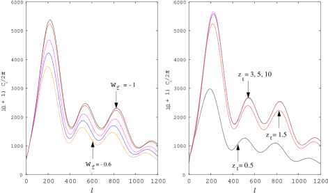
Figure 2: Variation of the $C_{\ell}$’s with $z_{t}$ and $w_{f}$. Left: The $C_{\ell}$ curves increase monotonically with decreasing $w_{f}$ starting with $-0.6$ (bottom), $-0.7,-0.8,-0.95$ and ending with $-1$ (top). The primary change is in the normalisation of the spectrum through the change in the ISW effect. Right: The $C_{\ell}$’s for $z_{t}=0.5$ (bottom), $1.5,3,5$ and $10$. The ISW contribution to the COBE normalisation changes very rapidly for small $z_{t}$ which allows for delayed acceleration. However, the CMB is insensitive to $z_{t}>3$ since the scalar field is dynamically irrelevant at those redshifts.

In addition, $z_{t}<2$ implies that the rapid change in $w$ can cause its own effect on the gravitational potential since the energy density of $Q$ is starting to dominate. This gives rise to an ISW effect purely due to the scalar field dynamics. We will see later that these two effects almost completely explain the behaviour of the likelihood curves in Fig.(4) which are very sensitive to small $z_{t}$ but exhibit a long tail for large $z_{t}$.

The other parameter of interest is $w_{f}$. This has a simple effect on the CMB. As $w_{f}$ decreases towards to $-1$ the universe starts to accelerate earlier and is accelerating more violently today. This alters the ISW effect which is important on large scales and which contributes to the COBE normalisation. The effect of $w_{f}$ is mainly then to amplify or supress the $\ell>50$ $C_{\ell}$’s by a more-or-less $\ell$-independent amount. This is evident in Fig. (2).

4.2 The matter power spectra

We now discuss the effect of $z_{t}$ and $w_{f}$ on the CDM and $Q$ power spectra. A key point is that the scalar field is very light both before and after the transition at $z_{t}$. This means that the associated Compton wavelength, $\sim(V^{\prime\prime})^{-1/2}$, of the $Q$ field is very large (as in standard quintessence models) for all times. This implies that no clustering occurs in the $Q$ field on small scales ($k>0.01h$ Mpc^-1).

After the transition the potential $V(Q)$ becomes even flatter (in order to obtain acceleration) and hence the Compton wavelength increases. This means that clustering now only occurs on the largest scales for $z<z_{t}$. This allows us an intuitive idea of the effect of $z_{t}$. As $z_{t}$ is increased, we see that the Compton wavelength effect forces clustering to occur only on larger and larger scales. However, this is actually only a fairly weak effect and the dominant variable is $w_{f}$.

The effect of $w_{f}$ on the $Q$ power spectrum is straight-forward: for fixed $z_{t}$, the closer $w_{f}$ is to $-1$, the less clustering occurs. Conversely, the closer $w_{f}$ is to $0$, the more clustering occurs. This is clear in the quintessence case from the work of Ma et al. (1999) which can be understood by rewriting the RHS of equation (5) in terms of the CDM density perturbation $\delta_{c}\equiv\delta\rho_{CDM}/\rho_{CDM}$ which becomes $\delta_{c}[(1+w_{f})\rho_{Q}]^{1/2}$. Clearly this driving term drops to zero as $w_{f}\rightarrow-1$.

For fixed $w_{f}$, increasing $z_{t}$ implies that the universe spends less time in the dust phase where $w=0$ and hence the long wavelengths of $\delta Q$ have less time to grow relative to the short wavelengths (that will not grow irrespective of the values of $z_{t}$ and $w_{f}$ ). This effect is clearly visible in Fig. 1 where we show the global best-fit CDM power spectrum with $z_{t}=1.5$ together with the best-fit to just the LSS data which has $z_{t}=6.5$ and hence less power on large scales. Similarly for fixed $z_{t}$, increasing $w_{f}$ towards zero allows more clustering on large scales relative to small scales.

An important point is that simply specifying $w_{f}=-1$ and $z_{t}>1000$ does not imply that the resulting model is the same as a $\Lambda$CDM model. While the transfer function $T(k)=1$ on all scales for $z<z_{t}$ if $w_{f}=-1$, this does not mean the initial power spectrum $P_{Q}(k)$ was zero, whereas $P_{\Lambda}(k)\equiv 0$ since $\delta\Lambda=0$ by definition. This is visible in the $C_{\ell}^{\prime}s$ of the left panel of figure (1). Both curves have $\Omega_{Q}=0.73$ and $w_{f}=-1$. They differ due to the fluctuations $\delta Q$ and the transition at $z_{t}=1.5$.

This means that despite the background dynamics being essentially equivalent for the two models for $z_{t}\rightarrow\infty$, the perturbations are not the same, and indeed one could consider adiabatic or isocurvature initial conditions for the $\delta Q$. Hence, simply showing that the recent dynamics of the universe favours $w=-1$ does not of itself, prove that the acceleration comes from the cosmological constant.

Tests sensitive to perturbations are also required. This may be particularly important in the case when the scalar field is non-minimally coupled to the spacetime curvature (see e.g. Perrotta & Bacciagalupi, 2001).

4.3 The SN1a data

To compare with the supernovae type Ia measurements we compute the luminosity distance:

$$d_{L}(z)=c(1+z)\int_{0}^{z}du/H(u)$$ (6)

from which $\Delta(m-M)=5[log_{10}(d_{L}(z))-log_{10}(d_{L_{0}}(z))]$ where $d_{L_{0}}=cz(z+2)/(2H_{0})$ is the empty-beam distance. We find that a step-function approximation to $w(z)$ is extremely accurate, due to the integral nature of the luminosity distance (see the dash-dotted line versus the short dashed line in figure (3)).

Figure (3) shows $\Delta(m-M)$ for a variety of models while figures (4) and (5) show the results of the likelihood analysis. Models with a very recent transition from deceleration to acceleration are favoured since they fit the highest $z$ supernova best, while still being consistent with the intermediate-$z$ supernovae at $z\sim 0.5$. Due to the large error bars, the constraints are weak, however. Furthermore, since the metamorphosis models are almost indistinguishable from standard $\Lambda$CDM models for $z<z_{t}$, we have only constraints on $z_{t}$ less than the redshift of the farthest supernova observed ($z\approx 1.75$).

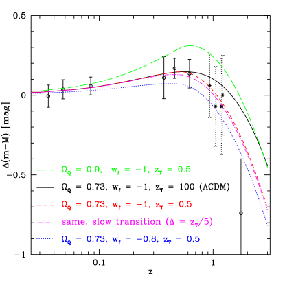
Figure 3: The redshift dependence of the luminosity distance (as magnitudes) minus an empty ($\Omega=0$) universe for four different metamorphosis models. The $z_{t}=0.5$ model fits the data best, mainly due to the single data point at $z=1.7$. The solid line effectively coincides with a $\Lambda$CDM model. The redshift-binned SN1a data is from Riess et al (2001); the four dashed data points are experimental and were not included in the fit.

The dependence on the other parameters is very much the same as for conventional dark energy models. Not surprisingly, we recover for $\Omega_{Q}$ vs $w_{f}$ the results of Turner and Riess (2001).

4.4 BBN constraints

Big-bang nucleosynthesis (BBN) primordial abundances depend sensitively on the expansion rate of the universe at the temperature $T=1$MeV which controls the neutron-proton ratio. Assuming that the quintessence field scales as radiation at nucleosynthesis Bean et al. (2001) set the limit of $\Omega_{Q}<0.045$ at $2\sigma$ at $T=1MeV$.

Since we assume the initial $w_{0}=0$, the scalar field scales as dust for $z>z_{t}$ and hence $\Omega_{Q}$ is dynamically negligible at nucleosynthesis which therefore provides no constraints on our parameters.

If we broadened our parameter set to include $w_{0}$ we would expect BBN to set joint limits on the parameters. In particular, for $w_{0}=1/3$ (radiation), the BBN data would favour large $z_{t}$, $w_{f}$ close to $-1$ and smaller $\Omega_{Q}$.

5 Results

Figures (4) and (5) show our main results through the marginalised 1-d and 2-d likelihoods for $(z_{t},w_{f},\Omega_{Q})$.

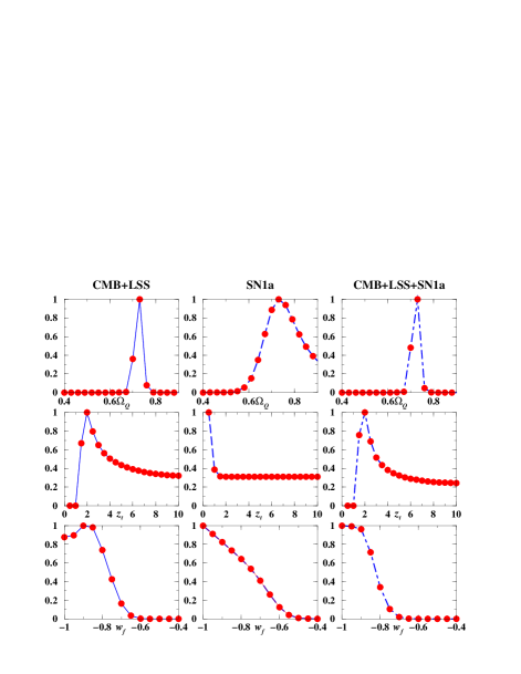
Figure 4: The marginalised 1-d likelihood plots for our variables $(\Omega_{Q},z_{t},w_{f})$. Left column: CMB + LSS, middle column: SN1a, right column: Total data set. Both the CMB and SN1a data favour a late transition (small $z_{t}$) due to the corresponding delay in cosmic acceleration. We computed these marginalised likelihoods using both integration and maximisation and the results were similar, as they should be for Gaussian likelihoods.

We do not show the likelihoods for CMB and LSS alone since the LSS provides only very weak constraints on $z_{t}$ (slightly preferring higher values) and $w_{f}$ (no constraints at all). It prefers an $\Omega_{Q}$ around $0.7$, consistent with the CMB likelihood. Due to these very weak results (and the consistent result for $\Omega_{Q}$), the likelihood for the CMB data looks just like the one for the combined CMB+LSS data.

The supernovae prefer (as explained in section 4.3) a low $z_{t}$, but its significance (stemming from only one supernova at $z>1$) is too weak to change the overall likelihood by much. The constraints on $\Omega_{Q}$ are weaker than for the other data sets, but consistent. Furthermore, the SN1a data prefers $w\approx-1$, which tightens the overall constraints on the equation of state somewhat, leading to $w<-0.8$ at the 1$\sigma$ level.

In Figs. (1) and (3) we show our best fits versus the current CMB, LSS and SN1a data and theoretical predictions of the standard $\Lambda$CDM model.

The $\chi^{2}$ values of the overall best fit model (with $w_{f}=-1.0$, $z_{t}=-1.5$ and $\Omega_{Q}=0.73$) are $33$ (CMB) + $36$ (LSS) + $4$ (SN1a), in total $73$. On the same parameter grid, the best fit $\Lambda$CDM model has $\Omega_{Q}=0.73$ as well. Its $\chi^{2}$ values are $40$ (CMB), $34$ (LSS) and $4$ (SN1a), in total $78$.

We used $49$ data points for the CMB, $48$ for the LSS and $7$ for the supernova data. We allowed a free overall model normalisation plus a bias/calibration uncertainty for each of the three LSS and the four CMB data sets. Our phenomenological model has three free parameters, while the $\Lambda$CDM models have only one. So in total we have approximately (neglecting correlations within the experiments as well as between them) $49+48+7-1-4-3-3=93$ degrees of freedom for our model, and $95$ dof for the $\Lambda$CDM models.

We can see that both groups of models are perfectly consistent with current data. Given the error bars of the data sets, the family of $\Lambda$CDM models is included in our phenomenological models for $w=-1$ and large $z_{t}$. The figures show that current data slightly prefers a low-$z$ phase transition, which is still true when taking into account that we have to add two degrees of freedom for pure $\Lambda$CDM models. On the other hand, the difference is too small to speak of a detection; assuming Gaussian errors and 3 “parameters of interest” ($\Omega_{Q}$, $w_{f}$, $z_{t}$), models with a $\Delta\chi^{2}$ of $5$ above the best-fit would formally be excluded at about 83%, hence somewhere between 1 and 2 $\sigma$.

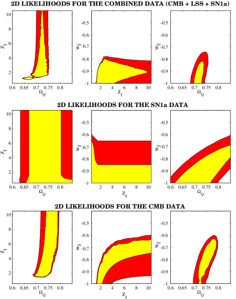
Figure 5: The marginalised 2-d likelihood plots for the combined CMB, LSS and SN1a data sets showing 1 and 2$\sigma$ contours defined as where the integral of the normalised two-dimensional likelihoods are equal to $0.68$ and $0.95$ respectively.

6 Conclusions and tests for late transitions

We have studied a phenomenological model in which the dark energy of the universe is described by a scalar field $Q$ whose equation of state $w$ undergoes a sudden transition (metamorphosis) from $w_{0}=0$ (dust) to $w_{f}<-0.3$ at a specific redshift $z_{t}$.

While similar to the quintessence paradigm in practical respects, the underlying philosophy is very different since we are interested in the possibility of detecting radical physics in the dark energy, such as the vacuum metamorphosis model (PR). We used the current CMB, large-scale structure (LSS) and supernovae (SN1a) data to constrain our phenomenological parameter space variables $(\Omega_{Q},z_{t},w_{f})$.

The CMB and SN1a data are sensitive to a transition if it occurs at low redshifts ($z_{t}<3$) due to the delay in the epoch at which cosmic acceleration can begin, relative to the standard $\Lambda$CDM models. We found that

• The global best-fit to the current data occurs for $z_{t}=1.5,w_{f}=-1.0$ and $\Omega_{Q}=0.73$ while the marginalised 1d likelihood for $z_{t}$ peaks at $z_{t}=2.0$. The best-fit model is consistent with the data and is a marginally better fit than the best $\Lambda$CDM model.

• The CMB provides the best constraints on the parameters, especially on $z_{t}$ due to the integrated Sachs-Wolfe effect (Fig. 4).

Is it possible to distinguish this metamorphosis from standard quintessence models?

This may be difficult since studies of quintessence favour similar values for $w_{f}$ and $\Omega_{Q}$ (Wang et al 1999, Bacciagalupi et al. 2002, Corasaniti & Copeland 2002) and $c_{s}^{2}=1$ in both cases (Erickson et al. 2001). Traditional methods to discover variation in $w$ based on the luminosity/area distance may be sufficient to discover transitions at $z_{t}<2$ but may be statistically inefficient in separating metamorphosis from standard quintessence since the distances effectively depend on the integral $\int w(z)dz$ (Maor et al. 2001).

An interesting alternative (Jimenez & Loeb 2001) is measurements of age differences in passively-evolving galaxies at different redshifts which in principle allow direct determination of $w(z)$ and a direct test of metamorphosis if $z_{t}$ lies in the epoch of galaxy formation ($z_{t}<5$).

Furthermore, future very high-precision measurements of the CMB at 1% or better might be able to detect the perturbations in the microwave background from the fluctuations in the scalar field itself, which would not be present in a smooth background component like a cosmological constant though separating this out from lensing and foreground contamination will be very difficult.

Finally, an intriguing possibility is that the rapid transitions studied here may provide a solution to the current impasse for quintessence models in explaining the varying-$\alpha$ data,viz: quintessence models can explain the apparent variation of $\alpha$ around $z\sim 1-3$ but cannot then simultaneously match the results of the Okun natural reactor (Chiba & Khori 2001) at $z\sim 0$. Detailed analysis of these issues is left to future work.

References

- [1] Amendola L., 2001, Phys. Rev. Lett., 86, 196.
- [2] Baccigalupi C., et al. , 2002, Phys. Rev. D65 063520.
- [3] Bean R., Hansen S. H., Melchiorri A., 2001, Phys. Rev. D64, 103508.
- [4] Bond J.R., Jaffe A.H., Knox L.E., 2000, Astrophys. J. 533, 19.
- [5] Caldwell R.R., Dave R., Steinhardt P. J., 1998, Phys. Rev. Lett. 80, 1582.
- [6] Carroll S., 1998, Phys. Rev. Lett. 81, 3067.
- [7] Chiba, T., Kohri, K., 2001, hep-ph/0111086.
- [8] Corasaniti P.S. and Copeland E.J., 2002, Phys. Rev. D 65 043004.
- [9] Croft R.A.C et al. , 2000, astro-ph/0012324.
- [10] Dienes, K.R., 2001, Nucl. Phys. B 611 146.
- [11] Erickson J. K. et al. , 2001, arXiv:astro-ph/0112438.
- [12] Ferreira P. G., Joyce M. 1998, Phys.Rev. D58 023503
- [13] Hamilton A.J.S, Tegmark M., 2000, astro-ph/0008392.
- [14] Halverson N.W. et al. , 2001 astro-ph/0104489.
- [15] Hill C.T. et al, 1989, Comments on Nucl. Part. Phys. 19, 25.
- [16] Holden D. J. and Wands D., 2000, Phys. Rev. D 61 043506.
- [17] Horvat, R. 2000, hep-ph/0007168.
- [18] Jimenez R., Loeb A., 2001, astro-ph/0106145.
- [19] Kamionkowski M, Buchalter A. 2000, astro-ph/0001045.
- [20] Lee A.T. et al. , 2001, Astrophys.J. 561, L1.
- [21] Ma C.P., Bertschinger E. Astrophys. J., 1995, 455, 7.
- [22] Ma C.P., Caldwell R.R., Bode P., Wang L., 1999, Ap.J. 521, L1.
- [23] Maor I., Brustein R., Steinhardt P.J., 2001, Phys.Rev.Lett.86, 6.
- [24] Miller J., Nichol R.C., Batuski D.J., 2001, Astrophys. J. 555, 68.
- [25] Netterfield C.B. et al. , 2001, astro-ph/0104460.
- [26] Padin S.T. et al. , Astrophys. J. 2001, 549, L1.
- [27] Parker L., and Raval A., 1999, Phys. Rev. D60, 123502.
- [28] Parker L., and Raval A. ,2000, Phys. Rev. D62, 083503.
- [29] Perlmutter S. et al. , 1999, Astrophys. J. 517, 565.
- [30] Perrotta F., Baccigalupi C., 2002, astro-ph/0201335.
- [31] Press, W.H., Ryden B.S., Spergel D.N., 1990, Phys. Rev. Lett. 64, 1084.
- [32] Riess A.G. et al. , 1998, Astronom. J. 116, 1009.
- [33] Riess A.G. et al. , 2001, Astrophys. J. 560, 49.
- [34] Sahni V., Habib S., 1998, Phys. Rev. Lett. 81, 1766.
- [35] Seljak U., Zaldarriaga M., 1996, Astrophys. J. 469, 437.
- [36] Tegmark M., Hamilton A.J.S, 1997, astro-ph/970219.
- [37] Tegmark, M. Zaldarriaga M., Hamilton, A. J. S., 2000, astro-ph/008167.
- [38] Tegmark M., Hamilton A.J.S., Xu Y., 2001, astro-ph/0111575.
- [39] Tocchini-Valentini D., Amendola, 2001,astro-ph/0108143.
- [40] Turner M.S., Riess A.G., 2001, astro-ph/0106051.
- [41] Verlinde E., Verlinde H., 2000, JHEP 0005, 034.
- [42] Verlinde E., 2000, Class. Quant. Grav. 17, 1277.
- [43] Wang X., Tegmark M., Zaldarriaga M., 2001, astro-ph/0105091.
- [44] Zaldarriaga M., Scoccimarro R. and Hui, L., 2001, astro-ph/0111230.