On rotationally driven meridional flows in stars

Abstract

A quasi-steady state model of the consequences of rotation on the hydrodynamical structure of a stellar radiative zone is derived, by studying in particular the role of centrifugal and baroclinic driving of meridional motions in angular-momentum transport. This nonlinear problem is solved numerically assuming axisymmetry of the system, and within some limits, it is shown that there exist simple analytical solutions. The limit of slow rotation recovers Eddington-Sweet theory, whereas it is shown that in the limit of rapid rotation, the system settles into a geostrophic equilibrium. The behaviour of the system is found to be controlled by one parameter only, linked to the Prantl number, the stratification and the rotation rate of the star.

1 Introduction

The study of the effects of rotation on the hydrostatic structure of a star is a long-standing problem (Eddington, 1925, Sweet, 1950). It is the key towards a better understanding of stellar evolution, and consequently, of the whole observable universe. The effects of rotation on the stellar evolution can be separated into two classes: effect on the contraction or expansion with time of various stellar regions and rotational mixing (of chemical species and angular momentum) through waves, instabilities and centrifugal driving of meridional motions. The effects of rotational mixing in stars was reviewed by Pinsonneault (1997) and can be directly observed (e.g. Li abundances and Li dip problem, MS turnoff, low-mass giants deep mixing …). Recent works by Maeder & Meynet (2000), or Chaboyer, Demarque & Pinsonneault (1995) for example, attempt to consider the effects of rotational mixing on stellar evolution through the resolution of one-dimensional stellar models using various ad-hoc parameterizations. These models are successful in explaining some aspects of the observations but their predictive power is sometimes limited.

In this paper I propose to approach the problem through a new path, which has different limitations and advantages thereby providing an interesting complement to the existing models. I choose to study the nonlinear effects of rotationally driven meridional flows on the angular-momentum distribution of a stellar radiative zone. In the limit of a slowly rotating star, this is equivalent to the well-known Eddington-Sweet problem. In the case of rapid rotation, this problem has received less attention; it can now be studied through the formalism introduced in this paper. This type of approach has been considered in the past (e.g. Tassoul & Tassoul (1983)); however, in previous works the nonlinearity of the angular-momentum transport processes was usually neglected mainly by assuming that the star was rotating nearly uniformly. As I shall show, this assumption is not self-consistent.

In Section 2, I present the equations for the hydrodynamic structure of a quasi-steady, laminar and axisymmetric radiative zone. The numerical results suggest a new scaling of the variables of the problem which can then be solved, in certain limits, analytically. The solutions are presented in Section 3. They provide the first self-consistent model of the effects of rotation on the centrifugal driving of meridional motions (assuming that the flow is a quasi-steady, laminar flow) and relies on one parameter only: the mean rotation rate of the star. The results are discussed in Section 4.

2 The model

I shall consider solar-type stars only and study their quasi-equilibrium structure under rotation. The overlying convection zone is affected by rotation mainly through the Coriolis distortion of the convective eddies. These effects are extremely complex; they are simply represented in this work through the rotation profile imposed by the convective zone to the underlying radiative zone. The radiative zone is assumed to be a stable, isotropic fluid with uniform dynamical viscosity $\mu$.

The steady-state structure of the rotating radiative zone is obtained by perturbing the hydrostatic equilibrium in the following way:

$$\rho_{\rm h}\mbox{\boldmath$u$}\cdot{\mathbf{\nabla}}\mbox{\boldmath$u$}=-{\mathbf{\nabla}}\tilde{p}-\rho_{\rm h}{\mathbf{\nabla}}\tilde{\Phi}-\tilde{\rho}{\mathbf{\nabla}}\Phi_{\rm h}+\mu{\mathbf{\nabla}}^{2}\mbox{\boldmath$u$}+\frac{1}{3}\mu{\mathbf{\nabla}}({\mathbf{\nabla}\cdot}\mbox{\boldmath$u$})\mbox{ ,}$$

$$\rho_{\rm h}T_{\rm h}\mbox{\boldmath$u$}\cdot{\mathbf{\nabla}}s_{\rm h}={\mathbf{\nabla}\cdot}(k{\mathbf{\nabla}}T)\mbox{ ,}\frac{\tilde{p}}{p_{\rm h}}=\frac{\tilde{\rho}}{\rho_{\rm h}}+\frac{\tilde{T}}{T_{\rm h}}\mbox{ ,}$$

$${\mathbf{\nabla}}^{2}\tilde{\Phi}=4\pi G\tilde{\rho}\mbox{ , }{\mathbf{\nabla}\cdot}(\rho_{\rm h}\mbox{\boldmath$u$})=0\mbox{ .}$$ (1)

where $p$ is the pressure, $T$ is the temperature, $\rho$ is the density, $\Phi$ is the gravitational potential, $\mbox{\boldmath$u$}=(u_{r},u_{\theta},u_{\phi})$ is the velocity field, $s$ is the entropy and $k$ is the thermal conductivity. As the system is axisymmetric and near-uniform rotation is not assumed, there is no need to work in a rotating frame. Quantities denoted with suffix h are derived from the non-rotating hydrostatic equilibrium equations, and perturbations to that state are denoted with tildes. The equations are linearized with respect to the background state (e.g. $\tilde{\Phi}\ll\Phi_{\rm h}$, $\tilde{\rho}\ll\rho_{\rm h}$), but the full nonlinearity is kept in the flow and in particular in the advection process $\mbox{\boldmath$u$}\cdot{\mathbf{\nabla}}\mbox{\boldmath$u$}$. This approach is rigorously correct provided the star is far from breakup (that is, when the mean ellipticity due to rotation is much smaller than unity). The steady-state assumption is valid provided the dynamical timescale of this system is short compared to the stellar evolution and spin-down timescales. This is not always necessarily the case, so that the direct applicability of the results presented in Section 3 must be checked a posteriori.

These equations must be supplemented with appropriate boundary conditions. Strictly speaking, correct boundary conditions would require a theory of the rotation and circulation in the convection zone to which the interior flows must be matched. Here, I shall simply assume that the forces maintaining the flow in the convection zone are so high that the angular velocity is unaffected by the flow in the underlying radiative zone, and is given by $\Omega_{\rm cz}(r,\theta)=\sum_{n=0}^{\infty}\Omega_{n}\mbox{ }{\rm cos}^{n}\theta$ (where $\theta$ is the co-latitude and $r$ is the radial variable). In addition, I suppose that the stresses affecting the meridional circulation are viscous-like. Since the effective viscosity in the convection zone is much greater than the viscosity in the radiative zone, it is not implausible that the continuity of stresses across the boundary imposes the constraints $\Omega=\Omega_{\rm cz}$, $\tau_{r,\theta}=r\partial(u_{\theta}/r)/\partial r+(1/r)\partial u_{r}/\partial\theta=0$ and $\partial\Omega/\partial r$ is continuous (and therefore null) at the interface. The inner core (for $r<r_{\rm in}$) is removed from the computational domain in order to avoid singularities. This core is impermeable and is assumed to rotate rigidly with angular velocity $\Omega_{\rm in}$ determined in such a way as to ensure a null angular-momentum flux through the boundary. Finally, the regions outside the domain of computation are assumed to satisfy ${\mathbf{\nabla}}^{2}\tilde{T}=0$ where $\tilde{T}$ vanishes both at $r=0$ and when $r\rightarrow\infty$ (since the inner core supports no fluid motion and the effective thermal conductivity in the convection zone is assumed to be much larger than in the radiative zone).

Using the assumption of axisymmetry, I reduce the momentum equation in (1) to:

$$\mbox{\boldmath$u$}\cdot{\mathbf{\nabla}}_{\xi}\left(\xi\mbox{ }{\rm sin}\theta u_{\phi}\right) = E_{\nu}{\rm D}^{2}\left(\xi\mbox{ }{\rm sin}\theta u_{\phi}\right)\mbox{ ,}$$

$$-\frac{1}{\rho_{\rm h}}\frac{\partial}{\partial z}\left(\rho_{\rm h}u_{\phi}^{2}\right) = -\frac{\mbox{ }{\rm sin}\theta}{\rho_{\rm h}}\left(\frac{\partial\rho_{\rm h}}{\partial\xi}\frac{\partial\tilde{\Phi}}{\partial\theta}-\frac{1}{\epsilon}\frac{\partial\tilde{\rho}}{\partial\theta}\right)$$ (2)

$$+ E_{\nu}{\rm D}^{2}\left(\xi\mbox{ }{\rm sin}\theta\omega_{\phi}\right)\mbox{ ,}$$

where $\mn@boldsymbol{\omega}={\mathbf{\nabla}\times}\mbox{\boldmath$u$}$ is the vorticity, $\xi=r/r_{\rm c}$ is the new normalized radial coordinate, $z$ is the normalized cylindrical coordinate that runs along the rotation axis, $E_{\nu}=\nu/r_{\rm c}^{2}\Omega_{\rm\star}$ is the Ekman number (where $\nu=\mu/\rho_{\rm h})$, and $\epsilon=r_{\rm c}^{2}\Omega_{\rm\star}^{2}(\partial\Phi_{\rm h}/\partial\xi)^{-1}$ is the ratio of the centrifugal to gravitational forces. The first of these equations simply describes angular momentum conservation, relating the advection term (LHS) to the diffusion term (RHS); the second equation is the azimuthal component of the curl of the momentum equation, commonly referred to in the geophysical literature as the ‘thermal wind equation’. In all these expressions the following normalizations have been applied: $\left[r\right]=r_{\rm c}$, $[u]=r_{\rm c}\Omega_{\rm\star}$, $[\tilde{\Phi}]=r_{\rm c}^{2}\Omega_{\rm\star}^{2}$, $[T]=1K$, $[\rho]=1$g/cm³, where $r_{\rm c}$ is the radius of the radiative zone and $\Omega_{\rm\star}$ is the typical rotation rate of the star. The operator ${\rm D}^{2}$ is defined as

$${\rm D}^{2}=\frac{\partial^{2}}{\partial\xi^{2}}+\frac{\mbox{ }{\rm sin}\theta}{\xi^{2}}\frac{\partial}{\partial\theta}\left(\frac{1}{\mbox{ }{\rm sin}\theta}\frac{\partial}{\partial\theta}\right)$$ (3)

The energy equation becomes, to first order in the thermodynamical perturbations

$$T_{\rm h}\frac{\sigma N_{\rm h}^{2}}{\Omega_{\rm\star}^{2}}\frac{\epsilon}{E_{\nu}}u_{r}={\mathbf{\nabla}}_{\xi}^{2}\tilde{T}$$ (4)

where $\sigma=\mu c_{\rm p}/k$ is the Prandtl number, and $N_{\rm h}$ is the background buoyancy frequency.

Finally, the equation of state can be combined with the radial and latitudinal components of the momentum equation to provide an expression for $\tilde{\rho}$:

$$\frac{1}{\rho_{\rm h}}\frac{\partial\tilde{\rho}}{\partial\theta}=\frac{\rho_{\rm h}}{p_{\rm h}}r_{\rm c}^{2}\Omega_{\rm\star}^{2}\left[\frac{\mbox{ }{\rm cos}\theta}{\mbox{ }{\rm sin}\theta}u_{\phi}^{2}-\frac{\partial\tilde{\Phi}}{\partial\theta}\right]-\frac{1}{T_{\rm h}}\frac{\partial\tilde{T}}{\partial\theta}$$ (5)

This expression is used in the thermal wind relation in (2) as well as in the latitudinal derivative of the Poisson equation

$$\frac{\partial}{\partial\theta}{\mathbf{\nabla}}^{2}\tilde{\Phi}=4\pi G\left[\frac{\rho^{2}_{\rm h}}{p_{\rm h}}r_{\rm c}^{2}\Omega_{\rm\star}^{2}\left(\frac{\mbox{ }{\rm cos}\theta}{\mbox{ }{\rm sin}\theta}u_{\phi}^{2}-\frac{\partial\tilde{\Phi}}{\partial\theta}\right)-\frac{\rho_{\rm h}}{T_{\rm h}}\frac{\partial\tilde{T}}{\partial\theta}\right]$$ (6)

The resulting equations (2), (4) and (6) combined with the mass continuity equation are solved for the unknowns $u_{r},u_{\theta},u_{\phi},\partial\tilde{\Phi}/\partial\theta$ and $\tilde{T}$.

3 Numerical and analytical results

The numerical study of the system presented in Section 2 was performed using the standard solar model calculated by Christensen-Dalsgaard et al. (1991) as the reference state. The imposed latitudinal shear was chosen to be that observed in the solar convection zone (with $\tilde{\Omega}_{\rm cz}=1-0.15\mbox{ }{\rm cos}^{2}\theta-0.15\mbox{ }{\rm cos}^{4}\theta$ in units of $\Omega_{\star}$). As the rotation rate $\Omega_{\star}$ is varied, it appears that only two parameters control the behaviour of the system: the Ekman number (which controls the boundary-layer behaviour and the flow velocities) and a new number

$$\lambda=\sigma N_{\rm h}^{2}/\Omega_{\rm\star}^{2}\mbox{ ,}$$ (7)

which controls the dynamics of the bulk of the radiative interior.

3.1 Slow rotation case: $\lambda\gg 1$

In the case of slow rotation, the numerical results suggest that $\tilde{T}$ and the poloidal components of the velocity $u_{r,\theta}$ scale with $E_{\nu}$ and $\lambda$ as:

$$\tilde{T}=\epsilon T_{\rm h}\overline{T}\mbox{ , }u_{r,\theta}=E_{\nu}/\lambda\overline{u}_{r,\theta}\mbox{ ,}$$ (8)

where the quantities with bars are the scaled quantities, of order of unity. It is also found that $u_{\phi}$ and $\tilde{\Phi}$ are always of order of unity, which is expected. Note that the scaling for the meridional motions is a local Eddington-Sweet scaling (see Spiegel & Zahn, 1992). Using this ansatz into the system of equations given in (1), an expansion in powers of $1/\lambda$ reveals that the angular-momentum balance is dominated to zeroth order by viscous transport through:

$${\rm D}^{2}(\xi\mbox{ }{\rm sin}\theta u_{\phi})=0\mbox{ ,}$$ (9)

which determines the angular velocity profile uniquely. Using this result in the first order equations provides a relation between the temperature and gravitational potential perturbations:

$$T_{\rm h}\frac{\partial}{\partial z}\left(\frac{1}{T_{\rm h}}u_{\phi}^{2}\right)=\mbox{ }{\rm sin}\theta\left(\frac{\partial\overline{T}}{\partial\theta}-\frac{\partial\ln T_{\rm h}}{\partial\xi}\frac{\partial\tilde{\Phi}}{\partial\theta}\right)\mbox{ ,}$$ (10)

$$\frac{\partial}{\partial\theta}{\mathbf{\nabla}}_{\xi}^{2}\tilde{\Phi}=-\frac{4\pi G\rho_{\rm h}r_{\rm c}}{g_{\rm h}}\left[\frac{\partial\ln p_{\rm h}}{\partial\xi}\left(\frac{\mbox{ }{\rm cos}\theta}{\mbox{ }{\rm sin}\theta}u_{\phi}^{2}-\frac{\partial\tilde{\Phi}}{\partial\theta}\right)+\frac{\partial\overline{T}}{\partial\theta}\right]\mbox{ ,}$$

which can be solved independently for $\overline{T}$ and $\partial\tilde{\Phi}/\partial\theta$. Finally, the temperature fluctuations lead to meridional motions through the energy advection-diffusion equation:

$$\overline{u_{r}}={\mathbf{\nabla}}^{2}_{\xi}\overline{T}\mbox{ .}$$ (11)

In Fig. 1, I show the results of the numerical solutions for the angular velocity profile and the meridional motions corresponding to a slowly rotating solar-type star (for which $\lambda\simeq 10^{4}$). The angular velocity profile is exactly the same as one obtained through solving $({\mathbf{\nabla}}^{2}\mbox{\boldmath$u$})_{\phi}=0$. The meridional flow velocities decrease strongly with depth and the streamlines follow a layered structure reminiscent of a Holton flow.

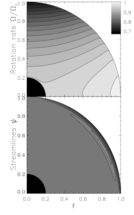
Figure 1: Numerical solution for a solar-type star rotating 100 times slower than the sun ($\lambda\simeq 10^{4}$). The quadrants show the radiative zone only. The upper panel shows the angular velocity, which is viscously dominated. The interior rotation rate is 0.957 times that imposed at the surface at the equator. The lower panel shows the streamlines (dotted lines represent a clockwise flow, and solid lines represent an anti-clockwise flow). The contours are logarithmically spaced.

3.2 Rapid rotation case: $\lambda\ll 1$

In the case of rapid rotation the correct scaling seems to be

$$\tilde{T}=\lambda\epsilon T_{\rm h}\overline{T}\mbox{ , }u_{r,\theta}=E_{\nu}\overline{u}_{r,\theta}\mbox{ .}$$ (12)

This time, I perform an asymptotic expansion in the small parameter $\lambda$. In this limit the temperature fluctuations are strongly damped by the rapid heat diffusion (as $\lambda\ll 1$ is equivalent to the small Prandlt number limit) and the system reaches an equilibrium that is determined by the zeroth order equations:

$$T_{\rm h}\frac{\partial}{\partial z}\left(\frac{1}{T_{\rm h}}u_{\phi}^{2}\right)=-\mbox{ }{\rm sin}\theta\frac{\partial\ln T_{\rm h}}{\partial\xi}\frac{\partial\tilde{\Phi}}{\partial\theta}\mbox{ ,}$$

$$\frac{\partial}{\partial\theta}{\mathbf{\nabla}}_{\xi}^{2}\tilde{\Phi}=4\pi G\frac{\rho^{2}_{\rm h}}{P_{\rm h}}\left[\frac{\mbox{ }{\rm cos}\theta}{\mbox{ }{\rm sin}\theta}u_{\phi}^{2}-\frac{\partial\tilde{\Phi}}{\partial\theta}\right]\mbox{ .}$$ (13)

These equations describe a geostrophic equilibrium, and can in principle be solved for $u_{\phi}^{2}$ and $\tilde{\Phi}$ alone. The solutions provide, to the next order in $\lambda$, an equation for the meridional flow through the advection diffusion balance:

$$\overline{\mbox{\boldmath$u$}}\cdot{\mathbf{\nabla}}_{\xi}\left(\xi\mbox{ }{\rm sin}\theta u_{\phi}\right)={\rm D}^{2}\left(\xi\mbox{ }{\rm sin}\theta u_{\phi}\right)\mbox{ ,}$$ (14)

and, finally, the temperature fluctuations through

$$\overline{u}_{r}={\mathbf{\nabla}}_{\xi}^{2}\overline{T}\mbox{ .}$$ (15)

The results of the numerical simulations for small $\lambda$ ($\lambda\simeq 10^{-2}$) are shown in Fig. 2.

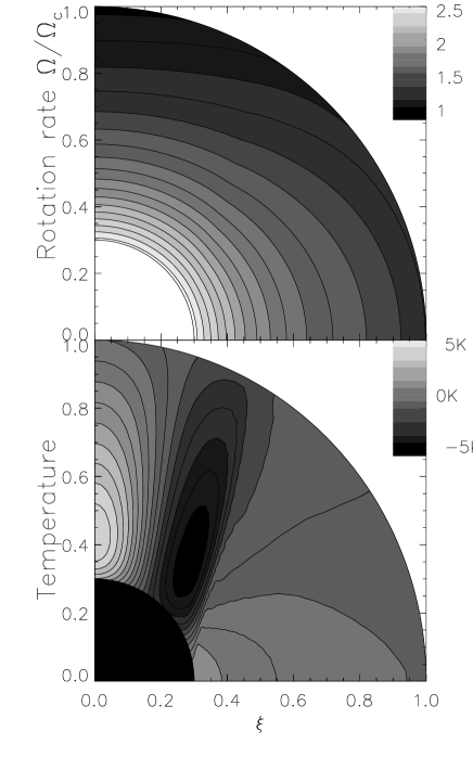
Figure 2: Numerical solution of the system (1) for a solar-type star rotating 10 times faster than the sun ($\lambda\simeq 10^{-2}$). The upper panel shows the angular velocity, which varies strongly with depth and the lower panel shows the temperature fluctuations. Note that even when the stellar oblateness is of order of $10^{-3}$, the temperature fluctuations remain of order of $10^{-6}$.

It is interesting to note that the radial shear is much larger than the latitudinal shear, which suggests to consider $\partial\Omega/\partial\xi\gg\partial\Omega/\partial\theta$ to perform a first analytical approximation. Similarly, I suppose that if $\Psi=\partial\tilde{\Phi}/\partial\theta$ then $\partial\Psi/\partial\xi\gg\partial\Psi/\partial\theta$. These approximations can be used into equations (2) and (6) to yield the system

$$\frac{1}{\xi^{2}}\frac{\partial}{\partial\xi}\left(\xi^{2}\frac{\partial\Psi}{\partial\xi}\right)=-\frac{4\pi Gr_{\rm c}^{2}\rho^{2}_{\rm h}}{p_{\rm h}}\left(\Psi+K\right)\mbox{ , }$$

$$\frac{\partial K}{\partial\xi}=\frac{\partial\ln T_{\rm h}}{\partial\xi}\left(\Psi+K\right)\mbox{ , }$$ (16)

where $K=\mbox{ }{\rm cos}\theta\xi^{2}\Omega^{2}$, which can easily be solved numerically for $K$ and $\Psi$. However, if the radiative zone is crudely approximated by a polytrope of index 3 then $T_{\rm h}\propto 1/\xi$ and $\rho_{\rm h}\propto 1/\xi^{3}$ between $\xi=0.3$ and $\xi=1$. This leads to

$$\frac{4\pi Gr_{\rm c}^{2}\rho^{2}_{\rm h}}{p_{\rm h}}\simeq\frac{\alpha_{0}}{\xi^{2}}\mbox{ and }\frac{\partial\ln T_{\rm h}}{\partial\xi}\simeq\frac{1}{\xi}\mbox{ . }$$ (17)

These expressions can be used in the system (16) to provide a homogeneous relation between $\Psi$ and $K$, which can (amongst other power law/oscillatory solutions) be solved analytically with $\Psi\simeq-K\simeq$ constant; this corresponds to $\Omega(\xi)\propto 1/\xi$. The comparison of this very simple analytical prediction with the results of the fully nonlinear numerical simulation is presented in Fig. 3, in the case where the convection zone shear is null and in the case where it is of order of 30% of the mean rotation rate. When the imposed shear is small, the analytical prediction provides a good approximation to the numerical results.

Figure 3: Comparison of the analytical prediction $\Omega(\xi)\propto 1/\xi$ (dotted line) with the numerical results (solid line) in the case of a solar shear (where the poles are rotating 30% slower than the equator) and in the case of no shear for a star with $\lambda\simeq 10^{-2}$. The no-shear case satisfies the spherical approximation intrinsically well, so that the analytical approximation is closer to the true solution in that case than in the sheared case. The discrepancy with the true solution increases near the core where the polytropic approximation to the equation of state is no longer valid.

3.3 Lower boundary problem

The numerical solutions for the angular velocity and the gravitational-field perturbation know little of the presence of a lower boundary; the meridional motions and the temperature fluctuations on the other hand seem to be strongly linked with the lower boundary conditions and may not represent what can be expected of a stellar radiative zone. In particular, the numerical simulations reveal the presence of an internal shear layer (related to the internal Stewardson layer in the Proudman spheres problem (Stewardson, 1966)), which is related to the presence of the impermeable lower boundary (and therefore mostly irrelevant to stellar hydrodynamics). This shear layer is reflected also in the temperature distribution (see Fig. 2). However, as the meridional flow and temperature distribution affect the angular velocity profile only to the next order in $\lambda$, it is possible to calculate the flow pattern as if there was no lower boundary using the simple ansatz $\Omega\propto 1/\xi$ into equation (14). Using the polytropic approximation again one can derive

$$\overline{\psi}=\xi\mbox{ }{\rm sin}^{2}\theta\left[\ln\left(\frac{1-\mbox{ }{\rm cos}\theta}{1+\mbox{ }{\rm cos}\theta}\right)\right]\mbox{ , }$$ (18)

where $\overline{\psi}$ is the scaled stream-function defined as $\overline{\mbox{\boldmath$u$}}=-{\mathbf{\nabla}\times}(\overline{\psi}/\xi\mbox{ }{\rm sin}\theta)$. This result suggests that in stars the dimensional radial component of the meridional flow varies as $u_{r}\propto\nu/r$ independently of the stellar rotation rate when $\lambda\ll 1$. Note that this scaling is compatible with the results of the work of Talon et al. (1997). As Busse (1981) claimed that rapidly rotating systems settle down to purely zonal flows in the inviscid case, it is not surprising to find that the typical timescale for steady circulation in this rapid-rotation limit is the very slow viscous timescale.

4 Discussion and conclusions

In this paper I analysed the consequences of rotation on the driving of meridional motions in stellar radiative zones. For a slowly rotating star, this problem has been studied by Eddington (1925) and Sweet (1950) who established that meridional motions are driven by stellar baroclinicity related to the rotation. For rapidly rotating stars, the problem has never been solved self-consistently. I have constructed a quasi-steady model of the rotating radiative zone of a solar-type (main-sequence) star which can be solved numerically for a wide range of rotation rates; through this numerical analysis I have been able to show that the effect of rotation on the stellar structure can be described with two parameters only: $\lambda=\sigma N_{\rm h}^{2}/\Omega_{\rm\star}^{2}$ and $E_{\nu}=\nu/r_{\rm c}^{2}\Omega_{\rm\star}$. The striking reduction of this complicated nonlinear problem to a rather simple form stems from the very close thermal advection-diffusion balance; this is intrinsically related to the very small Prandtl number typical of stellar radiative zones. In comparison, studies of the effect of rotation on stratified shear flows in the high-Prandtl-number limit reveal a very different behaviour (e.g. Clark et al., 1971).

The system approaches asymptotic limits in the case of fast rotation, $\lambda\ll 1$, and slow rotation, $\lambda\gg 1$. In both cases, interesting analytical reductions of the problem can be used. In the limit of slow rotation it was shown that typical flow velocities scale as the local Eddington-Sweet velocity, and the typical adjustment time of the system to the steady state is an Eddington-Sweet timescale (as expected). As a result, for molecular viscosities typical of solar-type stars it is unlikely that the system would ever relax to the steady state found here.

In the limit of rapid rotation ($\lambda\ll 1$), it was shown that the system settles into a geostrophic equilibrium; this can be achieved on a rather short timescale, which is linked with the generation and dissipation of inertial waves. As a result, this type of equilibrium is likely to be present in stars. The resulting rotation profile varies with radius roughly as $1/r$; the precision of this approximation depends on the degree of shear imposed by the convection zone. Assuming this simple profile for the angular velocity, the meridional motions can be deduced from angular-momentum conservation. The typical flow velocities in the steady-state are of order of $\nu/r_{\rm c}$, and are too slow to have any effect on material mixing. However, the continuous adjustment of the radiative zone to the stellar spin-down may lead to some significant mixing near the interface with the convection zone through the generation and dissipation of inertial waves. This can be studied self-consistently only through a time-dependent analysis of the flow, which is the subject of future work.

Of course, this analysis relies strongly on the fact that no dynamical effect save the rotation is present in the problem. The major corrections to take into account would be turbulent motion, magnetic field and chemical gradient. In regions where turbulent motions are expected (i.e. possibly near the edge of a convective zone, or in regions of strong shear) their effect could in principle be included in equation (1), provided a Reynolds-stress tensor for the microscopic motions is known. However, it is likely that the turbulent Prandtl number is much closer to unity, which would then render the analytical analysis obsolete (but not the numerical abilities of the code). If magnetic fields are present, either on large or small lengthscales, the whole dynamical structure of the star may be changed completely. A good example of this effect is well illustrated in the sun; observations reveal that the radiative interior is rotating nearly uniformly, as the shear imposed by the convection zone is suppressed within a very thin layer (the tachocline). Models exist (e.g. Gough & McIntyre, 1998) in which a small-amplitude, large-scale, fossil magnetic field within the radiative zone is able to impose uniform rotation throughout most of the interior. This type of fossil field is not unrealistic in any star. Finally, gradients in the mean molecular weight may also significantly alter the dynamics of the system by reducing or augmenting the effective buoyancy of the fluid, especially near boundaries with convective regions. Mestel (1953) has described how this effect may counterbalance the slow, rotationally driven motions, and Theado & Vauclair (2001) have argued that this effect may be essential in explaining the observed Li abundances in stars.

As a result, the rotation profile in rapidly rotating stars may not resemble that predicted in Section 3, but any observed discrepancy with the predicted model will be a clear signature of the effects discussed above.

Acknoledgments

I thank Professors D. O. Gough, L. Mestel and J.-P. Zahn for many fruitful discussions on this subject. I thank PPARC for financial support.

References

- [1] Brun, A. S., Turck-Chièze, S. & Zahn, J.-P., 1999, ApJ, 525, 1032
- [2] Busse, F. H., 1982, ApJ, 259, 759
- [3] Chaboyer, B., Demarque, P., & Pinsonneault, M. H., 1995, ApJ, 441, 865
- [4] Christensen-Dalsgaard, J., Gough, D. O. & Thompson, M. J., 1991, ApJ, 378, 413
- [5] Clark, A., Clark, P., Thomas, J. & Lee, N., 1971, JFM, 45,131
- [6] Eddington, A. S., 1925, Observatory, 48,73
- [7] Gough, D. O. & McIntyre, M. E., 1998, Nature, 394, 755
- [8] Maeder, A. & Meynet, G., 2000, Ann. Rev. Astron. Astrophys., 38, 143
- [9] Mestel, L., 1953, MNRAS, 113, 716
- [10] Pinsonneault, M. H., 1997, Ann. Rev. Astron. Astrophys., 35, 557
- [11] Proudman, I., 1956, JFM, 1, 505
- [12] Spiegel, E. A. & Zahn, J.-P., 1992, A&A, 265, 106
- [13] Stewartson, K., 1966, JFM, 26, 131
- [14] Sweet, E., 1950, MNRAS, 110, 548
- [15] Talon, S., Zahn, J.-P., Maeder, A., & Meynet, G., 1997, A&A, 322, 209
- [16] Tassoul, J.-L. & Tassoul, M., 1983, ApJ, 264, 298
- [17] Théado, S. & Vauclair, S., 2001, A&A, 375, 70