Modelling the Hubble Space Telescope Ultraviolet and Optical Spectrum of Spot 1 on the Circumstellar Ring of SN 1987A

Abstract

We report and interpret HST/Space Telescope Imaging Spectrograph (STIS) long-slit observations of the optical and ultraviolet (UV) ($1150-10270$ Å) emission-line spectra of the rapidly brightening Spot 1 on the equatorial ring of SN 1987A between 1997 September and 1999 October (days 3869 – 4606 after outburst). The emission is caused by radiative shocks created where the supernova blast wave strikes dense gas protruding inward from the equatorial ring. We measure and tabulate line identifications, fluxes and, in some cases, line widths and shifts. We compute flux correction factors to account for substantial interstellar line absorption of several emission lines.

Nebular analysis shows that optical emission lines come from a region of cool ($T_{e}\approx 10^{4}\mbox{ K}$) and dense ($n_{e}\approx 10^{6}\mbox{ cm}^{-3}$) gas in the compressed photoionized layer behind the radiative shock. The observed line widths indicate that only shocks with shock velocities $V_{s}<250\rm~{}km~{}s^{-1}$ have become radiative, while line ratios indicate that much of the emission must have come from yet slower ($V_{s}\mathrel{<\kern-10.00002pt\lower 3.87495pt\hbox{$\sim$}}135\rm~{}km~{}s^{-1}$) shocks. Such slow shocks can be present only if the protrusion has atomic density $n\mathrel{>\kern-10.00002pt\lower 3.87495pt\hbox{$\sim$}}3\times 10^{4}\mbox{ cm}^{-3}$, somewhat higher than that of the circumstellar ring. We are able to fit the UV fluxes with an idealized radiative shock model consisting of two shocks ($V_{s}=135$ and $250\rm~{}km~{}s^{-1}$). The observed UV flux increase with time can be explained by the increase in shock surface areas as the blast wave overtakes more of the protrusion. The observed flux ratios of optical to highly-ionized UV lines are greater by a factor of $\sim 2-3$ than predictions from the radiative shock models and we discuss the possible causes. We also present models for the observed ${\rm H}\alpha$ line widths and profiles, which suggests that a chaotic flow exists in the photoionized regions of these shocks. We discuss what can be learned with future observations of all the spots present on the equatorial ring.

1 Introduction

Supernova 1987A (SN 1987A) in the Large Magellanic Cloud provides an unprecedented opportunity to observe the birth and development of a supernova remnant. International Ultraviolet Explorer (IUE) observations (Fransson et al., 1989; Sonneborn et al., 1997) found narrow line emission about 80 days after the explosion, demonstrating the presence of circumstellar gas around SN 1987A. Images taken with the Hubble Space Telescope (HST) showed that this gas consists of an equatorial inner ring (radius $\approx 0.7$ light year, $n_{e}\sim 3\times 10^{3}-3\times 10^{4}\mbox{ cm}^{-3}$) and two outer rings ($\sim 3$ times the size of the inner ring, $n_{e}\mathrel{<\kern-10.00002pt\lower 3.87495pt\hbox{$\sim$}}2000\mbox{ cm}^{-3}$) tilted towards the observer at $\sim 45\arcdeg$ (Jakobsen et al., 1991; Wang, 1991; Plait et al., 1995; Burrows et al., 1995; Lundqvist & Fransson, 1996; Maran et al., 2000; Lundqvist & Sonneborn, 2001). The circumstellar ring system was excited by the ionizing radiation from the supernova during the shock breakout (Lundqvist & Fransson, 1991; Ensman & Burrows, 1992; Blinnikov et al., 2000). In the interacting winds model, the SN 1987A ring system is part of a bipolar shell around the supernova (Blondin & Lundqvist, 1993; Martin & Arnett, 1995; Link et al., 2001).

The first signal of ongoing interaction between the SN 1987A debris and the circumstellar gas was the rebirth of the supernova in X-ray (Beuermann, Brandt, & Pietsch 1994; Gorenstein, Hughes, & Tucker 1994; Hasinger, Aschenbach, & Trümper 1996) and radio (Staveley-Smith et al., 1992, 1993) wavelengths around day 1000. The size of the radio-emitting region indicated that the supernova debris expanded unimpeded at velocity $\mathrel{>\kern-10.00002pt\lower 3.87495pt\hbox{$\sim$}}35,000\rm~{}km~{}s^{-1}$ up to $\sim$ day 1000 before slowing down to $\approx 3500\rm~{}km~{}s^{-1}$ by the interaction (Gaensler et al., 1997; Manchester et al., 2001). The X-ray and radio observations have been explained as the interaction of the supernova ejecta with a rather dense ($n_{H}\approx 100\mbox{ cm}^{-3}$) H II region that separates the shocked stellar wind of the supernova progenitor from the denser gas of the inner ring (Chevalier & Dwarkadas, 1995; Borkowski et al., 1997a).

The “main event” of the birth of the Supernova Remnant 1987A (SNR 1987A) — the interaction between the supernova debris and the circumstellar rings — has been anticipated since the discovery of the circumstellar gas. Predictions of the time of the first contact ranged from 2003 (Luo & McCray, 1991) to $1999\pm 3$ (Luo, McCray, & Slavin 1994) to $2005\pm 3$ (Chevalier & Dwarkadas, 1995). There have been previous model predictions of radiation from this impact in X-rays (Suzuki et al., 1993; Masai & Nomoto, 1994; Borkowski et al., 1997b) and in the UV/optical (Luo et al., 1994). The first definitive sign of impact between the supernova blast wave and the inner ring was detected in the 1997 April HST/Space Telescope Imaging Spectrograph (STIS) spectral images as a blueshifted ($\sim-250\rm~{}km~{}s^{-1}$) ${\rm H}\alpha$ feature at position angle (PA) $\approx 30\arcdeg$ of the ring (Sonneborn et al., 1998). Subsequent analysis of the HST/Wide Field and Planetary Camera 2 (WFPC2) images taken in 1997 July showed that a point emission, located in projection at $88\%$ of the distance to the ring, was increasing in brightness over a wide range of wavelengths (Garnavich et al., 1997, 2001) and could be traced back to as early as 1995 March (day 2932) (Lawrence et al., 2000a). The position of the brightening spot, located just inside the edge of the inner ring, suggested that this is the result of an interaction of the supernova blast wave with an inward protrusion of the ring. This brightening spot, named Spot 1, has increased in flux by a factor of $\sim 10$ between 1996 and 1999 (Garnavich et al., 2001). With a number of new spots ($\sim 10$ in 2000 November) since then detected all around the inner circumstellar ring (Garnavich et al., 2000; Lawrence et al., 2000a), we are now witnessing the full birth of SNR 1987A.

We present here HST/STIS UV and optical spectroscopy of Spot 1 taken by the Supernova INtensive Study (SINS) collaboration up to day 4606 (1999 October 7). Results from an earlier (day 3869, 1997 September 27) STIS spectrum of Spot 1 have been presented in Michael et al. (2000). We describe the new observations and data reduction in §2 and report the results in §3. In §2.3 we describe a detailed method to determine the intrinsic fluxes and widths of a few UV lines, including the Si IV $\lambda\lambda$1394, 1403 and C IV $\lambda\lambda$1548, 1551 doublets, which are strongly affected by interstellar line absorption along the line of sight to the supernova.

Our working model (Figure Modelling the Hubble Space Telescope Ultraviolet and Optical Spectrum of Spot 1 on the Circumstellar Ring of SN 1987A ) for Spot 1, as well as the other spots, is that it is caused by the impact of the supernova blast wave with a dense inward protrusion of the ring (Michael et al., 2000). When the blast wave overtakes such an obstacle, slower shocks are transmitted into it. Since a range of densities is present in the ring, we expect (§4.1) that the transmitted shocks will have a range of velocities ($V_{s}\sim 100$ – $1000\rm~{}km~{}s^{-1}$). Not all of these shocks are responsible for the observed UV/optical emission from Spot 1 though. While some UV and optical line emission is produced right at the shock front, a much larger amount is produced if the shocked gas undergoes thermal collapse, i.e. the shock becomes radiative (§4.2). The time it takes for a shock to make this transition increases with its speed and decreases with its pre-shock density. Once the post-shock gas collapses, a shock becomes an extremely efficient radiator of UV and optical emission lines (§4.3). Therefore, while the range of possible velocities present in the ring is large, we are only observing the shocks which are slow and/or dense enough to have become radiative. Michael et al. (2000) confirmed this general picture and found that the observed line widths and line intensity ratios indicated the emission was formed by radiative shocks in the velocity range $\sim 100-250\rm~{}km~{}s^{-1}$ entering into a dense ($n_{0}\mathrel{>\kern-10.00002pt\lower 3.87495pt\hbox{$\sim$}}10^{4}\mbox{ cm}^{-3}$) gas.

Nebular analysis of the observed emission lines of Spot 1 (§5.1) suggests that the emission comes from a region of high density ($n_{e}>10^{6}\mbox{ cm}^{-3}$), This result confirms our picture that this emission comes from radiative shocks, which can compress the pre-shock gas by a factor $\mathrel{>\kern-10.00002pt\lower 3.87495pt\hbox{$\sim$}}100$. In §5.2, we model the UV line fluxes from Spot 1 between day 3869 and day 4587 with the one-dimensional steady state shock code of Cox & Raymond (1985). The observed UV fluxes are fitted well with models containing emission from two radiative shocks with $V_{s}=135$ and $250\rm~{}km~{}s^{-1}$. We propose two scenarios to interpret the observed increase of UV flux with time of Spot 1. In the first scenario the density of the obstacle is low enough so that the cooling times of shocks entering the obstacle are comparable to the age of the spot. The increase in UV line fluxes are then due primarily to the aging of the shocks as they develop thermally collapsed layers. In the second scenario, the obstacle is dense enough so that all the shocks cool almost immediately. The increased observed fluxes are instead attributed to an increasing surface area of shock interaction. While the second scenario fits the observed fluxes better, we suspect that the actual light curves probably manifest a combination of both effects. In §5.3 we discuss the observed line profiles and present simulated ${\rm H}\alpha$ line profiles based on simple geometric models for the shock interaction. In §6 we discuss what we have learned by comparing results of simplified shock models with the spectral observations, and describe how future observations may elucidate some unsolved problems. We summarize the main results in §7.

2 Observations and Data Reduction

The STIS observations of Spot 1 in both optical and UV wavelengths obtained by the SINS team are listed in Table 1. SN 1987A is located in a densely populated region of the LMC and appears to belong to a loose, young cluster region (Panagia et al., 2000). Target acquisition was complicated by the stars present near the supernova, especially Star 3, a Be star of $V\sim$ 16, at 1$\farcs$63 away and PA = 118°, and Star 2, a B2 III star of $V$ = 15.0, at 2$\farcs$91 away and PA = 318° from the supernova (Walborn et al., 1993; Scuderi et al., 1996). We decided to peak-up on the nearby star S2 (Walker & Suntzeff, 1990) and offset the telescope to center the aperture on Spot 1. We measured the required offset from the WFPC2 images (Garnavich et al., 2001). Due to the uncertainties in this measurement, Spot 1 was located at 0$\farcs$08 off the center of the slit for all observations taken before 1999 August. We reduced these data using the standard calibration files which assumed that the object was located at the center of the slit. We estimate that the offset from the center of the slit will cause us to underestimate the measured flux by $\mathrel{<\kern-10.00002pt\lower 3.87495pt\hbox{$\sim$}}5\%$ for the 0$\farcs$2 data, and by $\mathrel{<\kern-10.00002pt\lower 3.87495pt\hbox{$\sim$}}0.1\%$ for the 0$\farcs$5 data.

With each grating setting, we took multiple ($3-5$) observations centered at dithered positions 0$\farcs$5 apart along the slit. Cosmic rays (in the case of optical data) and hot pixels (in optical and UV data) were removed simultaneously when the dithered raw images were combined with the CALSTIS software developed by the STIS Investigation Definition Team at the Goddard Space Flight Center. Previous narrow-slit STIS spectra processed by the SINS team with this software showed that the flux calibration of far-UV (G140L) and near-UV (G230L) data agree to $\mathrel{<\kern-10.00002pt\lower 3.87495pt\hbox{$\sim$}}2\%$ for the overlapping region, while the agreement between near-UV (G230L) and optical (G430L) data is good to $\mathrel{<\kern-10.00002pt\lower 3.87495pt\hbox{$\sim$}}5\%$ (Baron et al., 2000; Lentz et al., 2001).

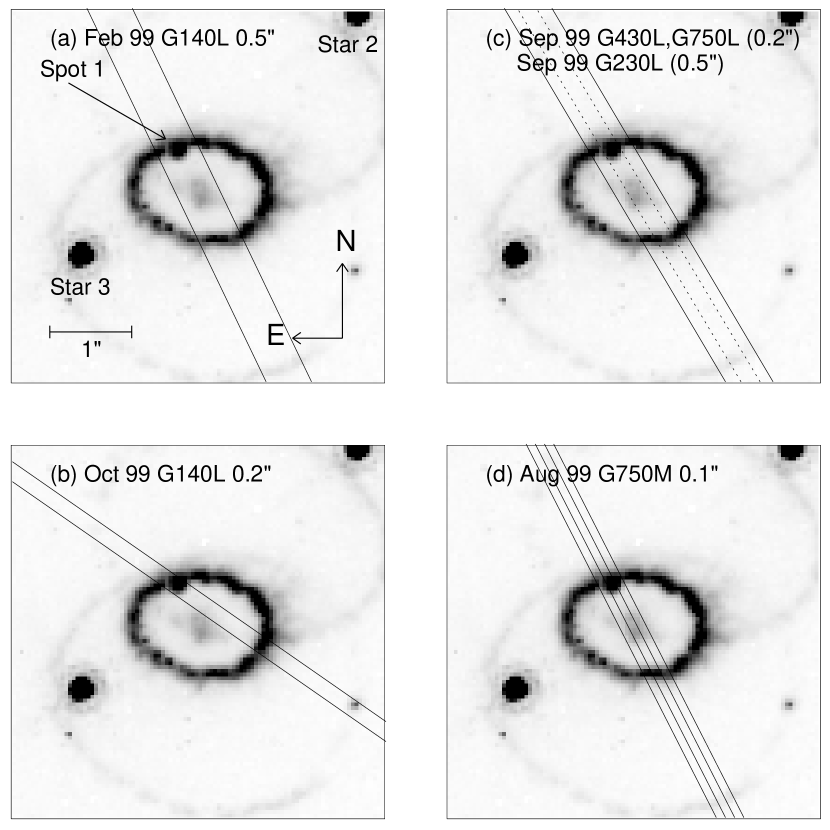
Figure 1: (a) Slit position of 1999 February 27 G140L 0$\farcs$5 observation plotted on the 1999 April 21 WFPC2 ${\rm H}\alpha$ image of SN 1987A. The image displayed is a $4\farcs 56\times 4\farcs 56$ square. (b) Same as (a), for the 1999 October 7 G140L 0$\farcs$2 observation. (c) Same as (a), for the 1999 September 17 G230L observation (solid) and for the 1999 September 3 G430L and 1999 September 18 G750L 0$\farcs$2 observations (dotted). (d) Same as (a), for the 1999 August 30 G750M 0$\farcs$1 observations. All three 0$\farcs$1 slit positions are plotted.

The location and orientation of the aperture positions are shown in Figure 1. For all but one of the observations, the slit was oriented (within $\pm 5\arcdeg$) along the axis connecting the center of the SN 1987A debris and Spot 1, which is located at a PA$=29\arcdeg$ on the inner ring (Garnavich et al., 2001). The only exception was the 1999 October G140L observation (Figure 1b), where the ($52\arcsec\times 0\farcs 2$) slit had a PA of 55$\arcdeg$ and did not pass through the center of the SN 1987A debris. In all observations, the Spot 1 spectrum overlapped with that from the adjacent segment of the inner circumstellar ring that was included within the STIS aperture. With an expansion velocity of $10.5\pm 0.3\rm~{}km~{}s^{-1}$ (Cumming & Lundqvist, 1997; Crotts & Heathcote, 2000), the ring was not resolved spectrally in any of the STIS observations reported here. In the optical data, the emission from the ring is the main source of background to the Spot 1 spectrum and will be discussed in §2.1 and §2.2.

Garnavich et al. (2001) measured the width of Spot 1 in WFPC2 images up to 1999 April 21 (day 4440) and showed that Spot 1 was unresolved in the data and was consistent with a point source at optical wavelengths. We compared the Full Width at Half-Maximum (FWHM) of Spot 1 emissions in our last STIS observations at 1999 September with those of point sources that were recorded in the data. We found that the FWHM of Spot 1 was $8\pm 6\%$ and $25\pm 9\%$ larger than a point source in the far-UV and optical wavelengths, respectively. The latter result is consistent with measurements by Lawrence et al. (2000b) with the 2000 May 1 (day 4816) STIS G750M spectroscopy, which suggests that Spot 1 is now moderately resolved in the HST data at optical wavelengths.

2.1 Low Resolution Optical Observations

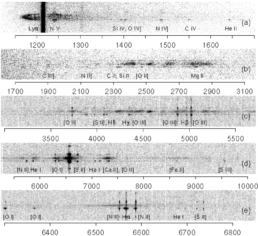
Figure 2: (a) Subsection of the 1999 October 7 STIS G140L (1425) spectral image showing the emission from Spot 1. The height of the image displayed is 6″ along the slit. (b) Same as (a), for the 1999 September 17 STIS G230L (2376) data. (c) Same as (a), for the 1999 September 3 STIS G430L (4300) data. (d) Same as (a), for the 1999 September 18 STIS G750L (7751) data. (e) Same as (a), for the 1999 August 30 STIS G750M (6581) data.

We extracted the low resolution optical spectrum of Spot 1 from the STIS G430L and G750L two-dimensional spectral images. Portions of the 1999 September G430L and G750L data taken with the 0$\farcs$2 slit are shown in Figures 2(c) and 2(d), respectively. The horizontal streaks near the center in the figure are broad emission lines from the inner supernova debris, which have a FWHM velocity $v_{\rm FWHM}\approx 2800\rm~{}km~{}s^{-1}$ (Wang et al., 1996; Chugai et al., 1997). For these data, the lower section of the spectral image is the combined Spot 1 and inner ring emission-line spectrum (hereinafter referred to as the Spot 1+North-Ring, or S1+NR, spectrum). At the kinematic resolution of the G430L and G750L grating settings ($\Delta V\approx 300-550\rm~{}km~{}s^{-1}$), neither the emission lines from Spot 1 [$v_{\rm FWHM}\approx 200\rm~{}km~{}s^{-1}$, Michael et al. (2000)] or those from the ring ($v_{\rm FWHM}\simeq 10\rm~{}km~{}s^{-1}$) are resolved. The upper section of the spectral image is the emission-line spectrum of the segment of the inner ring subsection that is in the slit and directly opposite that of Spot 1 (hereinafter referred to as the South-Ring, or SR, spectrum).

We measured the S1+NR and SR spectra in the G430L and G750L grating settings by integrating the $7-9$ rows of the image in which the emission-line spectra appeared. Emissions due to the diffuse LMC background in the Balmer lines, [O II] $\lambda\lambda$3727, 3729, and [O III] $\lambda\lambda$4959, 5007 are observed as images of the entire slit at those wavelengths in Figures 2(c) and 2(d). We subtracted the contribution of this diffuse emission from the Spot 1 spectrum by linear interpolation above and below the extracted rows. Since the subtracted LMC background was only a small fraction of the emission from Spot 1 ($<$2% for [O III] $\lambda$5007), this subtraction did not significantly increase the uncertainty of the estimated line fluxes.

We measured the flux of each emission line in the S1+NR and SR spectra by fitting a Gaussian to the line profile, allowing the net flux, width, and central wavelength to vary independently for each line. We estimated the background level from a linear fit over a 45-pixel region of the spectrum centered on the line in question but excluding any emission-line features. We fitted the line flux by minimizing the total $\chi^{2}$ in which the coefficients defining the line and the background were free parameters. Gaussian profiles gave satisfactory fits to all the line profiles. The reduced-$\chi^{2}$, or $\chi^{2}_{r}$, (the total $\chi^{2}$ divided by the number of degrees of freedom), of our line fits were within the range $0.8-2.8$, compared to the value of 1.0 for a statistically good fit. We computed the flux of each line and its error from the best-fit parameters and their associated uncertainties. We adjusted the statistical errors of all the line fluxes so that $\chi^{2}_{r}=1.0$ for all fits. In cases where two or more emission lines overlapped in wavelength, such as [O III] $\lambda$5007 + He I $\lambda$5016, and [Ar III] $\lambda$7136 + [Fe II] $\lambda\lambda$7155, 7172, we fitted the emission features with multiple Gaussians with the additional constraint that their wavelength separations were the known differences of laboratory wavelengths.

Only a subset ($\sim 1/3$) of the emission lines observed in the S1+NR spectrum also appeared in the SR spectrum. Therefore, we attributed entirely to Spot 1 the measured fluxes of emission lines that were seen in the S1+NR spectrum but not in the SR one. To subtract the NR spectrum from the S1+NR spectrum, we assumed that the fluxes of emission lines in the NR spectrum are equal to those in SR spectrum scaled by factors that are independent of time. This assumption is reasonable because the rate of flux decrease around the ring has been shown to be relatively constant around the ring (Plait et al., 1995; Lundqvist & Sonneborn, 2001). We estimated the scale factors by examining archival WFPC2 emission-line images in ${\rm H}\alpha$, [O III] $\lambda$5007, and [N II] $\lambda$6583 obtained in 1994 February and 1994 September, before Spot 1 appeared. We measured flux ratios $f(NR)/f(SR)$ of 1.2, 1.1, and 1.3, respectively from the ${\rm H}\alpha$, [O III] $\lambda$5007, and [N II] $\lambda$6583 images. We used the ${\rm H}\alpha$ scale factor for the Balmer lines. While we used the [O III] $\lambda$5007 factor for the [O III] $\lambda\lambda$4363, 4959, 5007 lines, and likewise for the [N II] lines, we recognized the increase in systematic errors in the measured Spot 1 fluxes of [O III] $\lambda$4363 and [N II] $\lambda$5755 because these lines are more temperature sensitive than the other lines. For all remaining emission lines, such as [S II] and [Ne III], we assumed a scale factor of $1.2\pm 0.1$ in order to subtract the NR spectrum.

In addition to the 0$\farcs$2 data sets described above, we obtained one observation of Spot 1 with the 0$\farcs$5 slit and the G750L grating setting. As before, we extracted the combined S1+NR spectrum by integrating the 6 rows of the image where the emission lines appeared. For the emission lines produced predominantly by Spot 1, such as He I $\lambda$6678 and [Ar III] $\lambda$7135, we measured the S1 fluxes by fitting the line emissions with single Gaussian profiles. For the lines where emission from both S1+NR were apparent, such as [N II] $\lambda$5755 and [O I] $\lambda$6300, we estimated the contribution of the NR flux to the S1+NR flux from a linear interpolation of the NR emission-line flux adjacent to Spot 1 in the slit. After subtracting this background, we fitted the remaining S1 emission lines with Gaussian profiles. The uncertainties in the background ring flux estimated in this procedure resulted in larger systematic errors in the estimated Spot 1 line fluxes for this observation.

2.2 Medium Resolution Optical Observations

A medium resolution optical spectrum was taken on 1999 August 30 (UT, 4368.0 days since explosion) with a 0$\farcs$1 slit and the G750M (6581) grating setting ($6295-6867$ Å). With a spectral resolution of $\Delta V\simeq 50\rm~{}km~{}s^{-1}$, emission lines from Spot 1, with $v_{\rm FWHM}\approx 200\rm~{}km~{}s^{-1}$ (Michael et al., 2000), were resolved in the data, while the emission from the unshocked inner ring, with $v_{\rm FWHM}\simeq 10\rm~{}km~{}s^{-1}$, remained unresolved. Three observations of 7800 seconds each were taken at three parallel slit positions, pointed so that the middle slit position was centered on Spot 1 and the two other slit positions were immediately adjacent [cf. Figure 1(d)]. Therefore the observation covered a segment of the ring of length 0$\farcs$3.

With the crowded stellar field near SN 1987A, we did not execute the acquisition-peakup exposure for these 0$\farcs$1 slit observations as suggested by the HST/STIS operation manual (Leitherer et al., 2000). Instead all three adjacent slit positions were placed on Spot 1 by blind offsets. Therefore we cannot apply the standard pipeline data reduction procedures to process these data. To determine the fluxes of emission lines from Spot 1, we first removed the wavelength-dependent aperture throughput correction function in the pipeline data for each 0$\farcs$1 slit spectrum. We then summed the fluxes from the three 0$\farcs$1 slit positions, and multiplied the total flux by a new aperture correction function for an equivalent 0$\farcs$3 slit, calculated by interpolating the pipeline corrections for the 0$\farcs$1, 0$\farcs$2, and 0$\farcs$5 slits. For ${\rm H}\alpha$, the aperture correction led to a $\simeq 20\%$ decrease of flux over the sum of the fluxes measured in the three slit positions. We calculated the corresponding 1$\sigma$ errors by combining the individual errors in quadrature.

A section of the spectral image from the middle slit position is shown in Figure 2(e). Again, the central horizontal streak is emission from the SN 1987A debris. Emissions from the inner ring at the two positions where the ring intersected with the slit aperture were observed in [O I] $\lambda\lambda$6300, 6364, ${\rm H}\alpha$, [N II] $\lambda\lambda$6548, 6583, and [S II] $\lambda\lambda$6717, 6731. In the lower section of the spectral image, emission from the stationary inner ring overlapped with the broadened emission from Spot 1. Again, the major source of contamination the Spot 1 spectrum is the emission from the inner circumstellar ring within the 0$\farcs$1 slit. As described by Michael et al. (2000), we fit all the Spot 1 emission features with Gaussian functions. Emission from the stationary ring dominated the spectral profile near zero velocity ($\sim\pm 50\rm~{}km~{}s^{-1}$) and was excluded from the fit. The majority of the line profiles could be fitted well with Gaussian profiles, such as the fit to the [N II] $\lambda$6583 line emission shown in Figure 3. The sole exception was the ${\rm H}\alpha$ line profile, where the signal was strong enough to show noticeable departures from a Gaussian profile, as we shall discuss further in §5.3.

2.3 Low Resolution UV Observations

We obtained low resolution UV spectra of Spot 1 with the G140L and G230L grating settings. Michael et al. (2000) have already presented results from the first G140L far-UV observations in 1997 September 27 taken with the 0$\farcs$5 slit. We detected emission lines from Spot 1 in N V $\lambda\lambda$1239, 1243, Si IV $\lambda\lambda$1394, 1403, O IV] $\lambda$1400, N IV] $\lambda\lambda$1483, 1487, C IV $\lambda\lambda$1548, 1551, and He II $\lambda$1640. We detected the same set of emission lines in 1999 February 27, observing again with the 0$\farcs$5 slit. In 1999 October 7, observing with the 0$\farcs$2 slit, we also detected the C II $\lambda$1335 multiplet, [Ne IV] $\lambda$1602, and O III] $\lambda\lambda$1661, 1666. Figure 2(a) shows a section of the spectral image from this observation. Radiation from Spot 1 is evident in the lower portion of the image whereas only faint line emission from the inner circumstellar ring can be seen in the upper half of the displayed image. The broad ($\sim\pm 15,000\rm~{}km~{}s^{-1}$) ${\rm Ly}\alpha$ radiation comes from the reverse shock from the interaction between the supernova debris and the H II region located inside of the equatorial ring (Sonneborn et al., 1998; Michael et al., 1998a, b). Fluxes of UV line emission from the inner ring are much less than those from Spot 1 and make a negligible contribution to the measured fluxes. This is also the case for the near-UV emission lines measured in the 1999 September 17 G230L 0$\farcs$2 observation, shown in Figure 2(b).

We measured the far-UV and near-UV spectra of Spot 1 from the G140L and G230L data, respectively, by procedures similar to those we described in §2.1. We fitted emission lines with Gaussian profiles and linear backgrounds, except for the broad ${\rm Ly}\alpha$ emission underlying the N V $\lambda\lambda$1239, 1243 doublet which we fitted with a quadratic function. We fitted the two components of close doublets such as N V $\lambda\lambda$1239, 1243, C IV $\lambda\lambda$1548, 1551, O III] $\lambda\lambda$1661, 1666, N II] $\lambda\lambda$2139, 2143, and Mg II $\lambda\lambda$2796, 2803 with Gaussians constrained to have fixed doublet separations, identical widths, and line ratios dictated by their oscillator strengths. At the resolution of the G140L grating setting, the Si IV $\lambda$1403 emission of the Si IV $\lambda\lambda$1394, 1403 doublet is blended with the O IV] $\lambda$1400 multiplets. We fit the combined Si IV and O IV] feature with multiple Gaussians, requiring the Si IV doublet to meet the same constraints as the other close doublets.

The observed fluxes of a few UV lines, such as Si IV $\lambda\lambda$1394, 1403 and C IV $\lambda\lambda$1548, 1551, were reduced by interstellar line absorption. We describe our procedure for correcting for this absorption in §3.3 below.

3 Data

3.1 Optical Emission Line Fluxes

Table 2 lists the measured Spot 1 optical emission line fluxes, including previously published results from the 1998 March 7 (day 4030) data by Michael et al. (2000) and 1$\sigma$ upper flux limits for the [O II] $\lambda\lambda$3726, 3729, and [N I] $\lambda\lambda$5198, 5200 doublets. The 1$\sigma$ errors tabulated are only statistical errors. Systematic effects, such as fringing for the G750L data towards the near-IR region ($\lambda>8500$ Å, Leitherer et al. 2000), might contribute additional uncertainties to the measured fluxes.

The tabulated fluxes have been dereddened with E($B-V$) of 0.16 (Fitzpatrick & Walborn, 1990) and the extinction law of Cardelli et al. (1989) with an assumed R_V of 3.1. In the optical band the differences between the LMC extinction law and the Galactic law are negligible at low color excess (Fitzpatrick, 1999). The interstellar extinction correction applied is listed in the last column of Table 2.

Spot 1 was observed in many neutral and lowly ionized species in the optical wavelengths. We did not detect any coronal lines such as [Fe X] $\lambda$6375. Most of the line fluxes increased with time at a rate comparable to that measured from WFPC2 photometry (Garnavich et al., 2001). At the low spectral resolution of both the G430L and G750L observing modes ($R=\lambda/\Delta\lambda=530-1040$), definitive line identification remained a problem, especially for the [Fe II] emission lines. The Fe line identifications in Table 2 are based upon the modeling of the Spot 1 Fe lines in Pun et al. (2002, in preparation). Moreover, several lines were blended. Table 2 lists possible contributing species and, in the case of [Fe II] lines, different multiplets. In contrast, line blending is not a problem in the medium resolution G750M ($R\approx 6000$) data.

Fluxes in [O I] $\lambda\lambda$6300, 6363 and He I $\lambda$6678 were measured with the low resolution G750L and medium resolution G750M gratings in 1999 September within 17 days of each other. The two measurements agreed within uncertainties for the [O I] doublet. The two results differed by $\sim 50\%$ for the low S/N He I $\lambda$6678 data, but were also within the noise level. This difference is probably a good indication of the detection limits of such faint lines.

3.2 Optical Emission Line Widths

For the medium resolution G750M observations, apart from the line fluxes, we were also able to measure the peak emission velocities ($V_{0}$) and the widths ($V_{\rm FWHM}$) of the emission lines from the profile fits. Table 3 lists the results. The peak emission velocity measurements have been adjusted for the SN 1987A heliocentric velocity of $+286\rm~{}km~{}s^{-1}$ (Wampler et al., 1989). The 1998 March 0$\farcs$2 G750M results have also been adjusted for the off-center position of Spot 1 within the aperture (cf. §2). The main uncertainties in the measurements of both $V_{0}$ and $V_{\rm FWHM}$ are due to the contributions by emission from the stationary circumstellar ring, which dominated the emission by Spot 1 near zero velocity for many species (cf. Figure 3). The errors due to this contribution are generally smaller for the 1999 August 0$\farcs$1 observations than the 1998 March 0$\farcs$2 ones.

For all emission lines, the line centroids from Spot 1 were blueshifted, with peak velocity $V_{0}$ lying within the range $-40$ to $-10\rm~{}km~{}s^{-1}$. This result is consistent with the overall physical picture in which Spot 1 is located on the near side of the equatorial ring (Sonneborn et al., 1998) and the shock entering Spot 1 is moving towards the observer. We found no evidence that the peak velocity $V_{0}$ of Spot 1 varied with time.

Most emission lines had widths (FWHM) within the range $\sim 150-180\rm~{}km~{}s^{-1}$, except [N II] $\lambda$6583 and ${\rm H}\alpha$, which had a slightly greater width, $V_{\rm FWHM}\mathrel{>\kern-10.00002pt\lower 3.87495pt\hbox{$\sim$}}200\rm~{}km~{}s^{-1}$. We detected no measurable change with time of the line widths except for ${\rm H}\alpha$ and [N II] $\lambda$6548. For ${\rm H}\alpha$, the emission profile from the second observation in 1999 August could no longer be fit well by a single Gaussian (to be discussed further in §5.3). The width of the [N II] $\lambda$6548 emission, measured in 1999 August was 1.5 times greater than that measured in 1998. However, we are inclined to attribute this increase to systematic error, since we detected no such increase in the other [N II] component at 6583 Å, where the line fluxes were $\sim 3$ times stronger.

3.3 UV Emission Lines

3.3.1 Interstellar Line Absorption

Near the time of outburst, interstellar absorption lines of C II $\lambda$1335 multiplet, Si IV $\lambda\lambda$1394, 1403, C IV $\lambda\lambda$1548, 1551, and Mg II $\lambda\lambda$2796, 2803 were observed in the UV continuum of SN 1987A with IUE operating in the high resolution ($\Delta V\approx 30\rm~{}km~{}s^{-1}$) echelle mode (Blades et al., 1988; Welty et al., 1999). For each line, the dominant absorption component was centered at $+281\rm~{}km~{}s^{-1}$, near the SN 1987A heliocentric velocity of $+286\rm~{}km~{}s^{-1}$ (Wampler et al., 1989), and had a FWHM of $\sim 80\rm~{}km~{}s^{-1}$. Therefore, narrow emission lines ($v_{\rm FWHM}\simeq 10\rm~{}km~{}s^{-1}$) from the inner circumstellar ring from these species are completely blocked by the interstellar absorption (Fransson et al., 1989), as demonstrated by the absence of Si IV and C IV emission lines from the ring in Figure 2(a).

Emission lines from Spot 1, with $V_{\rm FWHM}\approx 200\rm~{}km~{}s^{-1}$, are not totally blocked by these interstellar absorption lines, as correctly predicted by Luo et al. (1994). However, the line profiles are altered and the observed fluxes are reduced substantially. Therefore, we must correct the measured C II, Si IV, C IV, and Mg II emission line fluxes to account for this absorption. The appropriate correction factors depend on the profile shapes of both the Spot 1 emission and the intervening absorption. To make this correction, we assumed that the UV emission lines from Spot 1 had Gaussian profiles with the same parameters as the optical lines as measured in the medium resolution optical data (§2.2). We then estimated the amount of flux reduction in the UV emission lines by multiplying the assumed Gaussian profiles by the absorption profiles seen in the IUE data. The corresponding flux correction factors for the various emission lines are shown in Figure 4(a). The correction factor is greatest for the Mg II $\lambda\lambda$2796, 2803 doublet, where the interstellar absorption is almost completely saturated between $-50$ and $+300\rm~{}km~{}s^{-1}$.

The flux correction factor due to interstellar absorption is sensitive to the assumed widths ($V_{\rm FWHM}$) and peak ($V_{0}$) velocities of assumed line profiles from Spot 1. Figure 4(b) illustrates this dependence for the important case of C IV $\lambda\lambda$1548, 1551. We see that the flux correction factor increases moderately with decreasing $V_{\rm FWHM}$ for $V_{\rm FWHM}>200\rm~{}km~{}s^{-1}$, but becomes very sensitive to both $V_{\rm FWHM}$ and $V_{0}$ for $V_{\rm FWHM}<150\rm~{}km~{}s^{-1}$.

As we shall discuss below in §5.3, the peak velocities and widths of the emission lines from Spot 1 depend on the detailed geometry and hydrodynamics of the shocks entering the spot, which are unknown. It is not obvious that the optical and UV emission lines should have the same peak velocities and widths. However, in the plane-parallel shock model that we describe in §4, we found that the peak velocities of emission from Spot 1 were almost identical in both the UV and optical wavelengths. Therefore, we used the measured peak Spot 1 velocities from the medium resolution optical observations, $V_{0}=-30\pm 15\rm~{}km~{}s^{-1}$ (cf. Table 3), to estimate the flux correction factors to account for interstellar absorption of the UV emission lines.

3.3.2 Widths of the UV Emission Lines

The far-UV emission lines from Spot 1 are poorly resolved at the spectral resolution of the G140L grating ($\Delta V\approx 250\rm~{}km~{}s^{-1}$ at 1500 Å). For these lines, we attempted to establish the relation between the actual and observed widths through Monte Carlo simulations. For the simulations, we assumed that the intrinsic Spot 1 emission lines had (i) a Gaussian shape with FWHM as a variable parameter, (ii) emission peaked at $-30\rm~{}km~{}s^{-1}$, and (iii) flux ratio of the doublets dictated by their oscillator strengths.

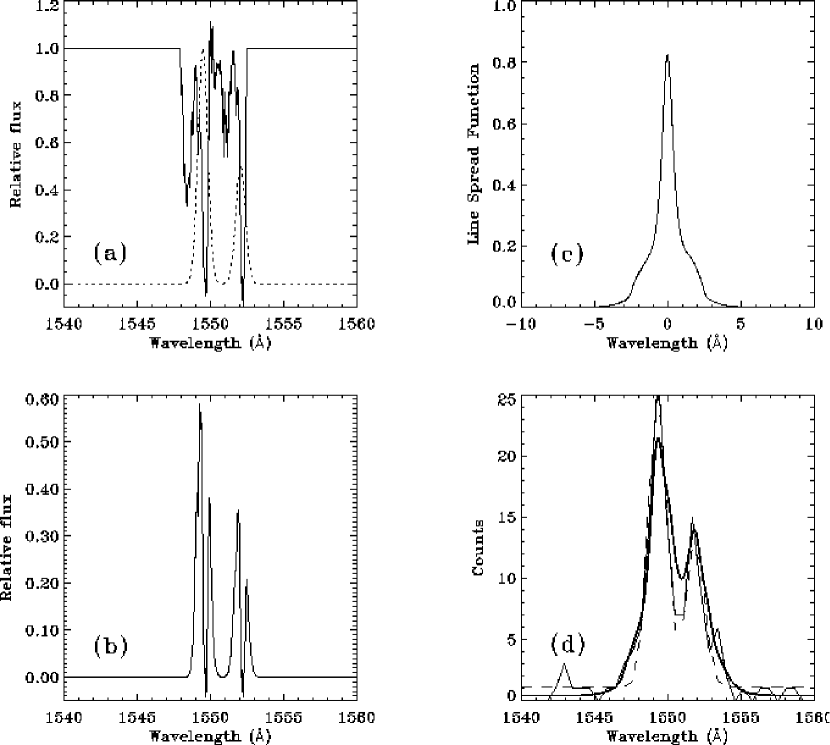
Figure 5: (a) The IUE high dispersion spectrum of the C IV $\lambda\lambda$1548, 1551 absorption lines (solid), overlayed with a model Gaussian Spot 1 line profile of the C IV emission line (dots). The FWHM width of the model profile is $150\rm~{}km~{}s^{-1}$ and it peaks at $-30\rm~{}km~{}s^{-1}$ with line ratio $I$(1548)/$I$(1551) = 2:1. (b) The model C IV Spot 1 spectrum after the interstellar line absorption. (c) The LSF of STIS/MAMA G140L grating for the 0$\farcs$2 aperture at 1500 Å. (d) The model “observed” spectrum after convolving the model profile after absorption with the line spread function (thick). Example of a Monte-Carlo generated line profile of the C IV doublet, normalized to the integrated counts of the 1999 October data, is also shown (solid), along with the best-fit double Gaussian function to this profile (dash). In this example, the best-fit $V_{\rm FWHM}=281\rm~{}km~{}s^{-1}$.

The dotted curve in Figure 5(a) shows a model C IV $\lambda\lambda$1548, 1551 profile, assuming $V_{\rm FWHM}=150\rm~{}km~{}s^{-1}$ and line flux ratio $I(1548)/I(1551)=$ 2:1. The solid curve shows a subsection of the high resolution IUE spectrum with the absorption line profile for the C IV doublet. For each input FWHM, we multiplied the model input emission line by the measured IUE absorption spectrum. Figure 5(b) shows a typical result. We convolved this profile with the line-spread function (LSF) of the detector for the slit aperture of the data set. The LSF for each emission line was interpolated from the measured LSFs at 1200 Å, 1500 Å, and 1600 Å. The LSF typically has a narrow peak ($\sim 1.5$ pixel) and a broad wing that extends to $\sim 10$ pixels on either side of the peak (Leitherer et al., 2000). Figure 5(c) shows a typical example of the LSF for the G140L grating at 1550 Å with the 0$\farcs$2 aperture.

For each emission line, we normalized the resulting convolved profile to the photon counts for each observation. The thick solid curve in Figure 5(d) shows the normalized model C IV line profile for the 1999 October observation. We constructed a simulated observed profile (the thin solid curve in Figure 5d) by applying random noise to the model profile and sampling it at the spectral resolution of the G140L grating. Finally, we fitted the simulated profile with Gaussians in the same way as the real data. The dotted curve in Figure 5(d) shows such a fit.

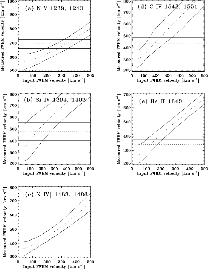
Figure 6: Monte Carlo results of the relation between the intrinsic Spot 1 emission width and the measured widths from Gaussian fittings for the 1999 October G140L 0$\farcs$2 observations in (a) N V $\lambda\lambda$1239, 1243; (b) Si IV $\lambda\lambda$1394, 1403; (c) N IV] $\lambda\lambda$1483, 1486; (d) C IV $\lambda\lambda$1548, 1551; and (e) He II $\lambda$1640.

For each input model FWHM velocity, we ran 10000 simulations and generated an array of the corresponding observed line widths. Figure 6 shows the median and the 68.3% (1$\sigma$) upper and lower limits of the array plotted against the model input widths of the various observed emission lines. We use these results to convert the observed line widths from the STIS data, shown as horizontal lines in Figure 6, to the intrinsic widths of the lines emitted by Spot 1.

We did not attempt to model the near-UV G230L data in this way because the spectral resolution for this grating setting ($\Delta V\approx 450\rm~{}km~{}s^{-1}$ at 2500 Å) was too low for such a procedure to yield useful results.

For all emission lines except the N V doublet, we found a 1$\sigma$ upper limit of ${\rm FWHM}\mathrel{<\kern-10.00002pt\lower 3.87495pt\hbox{$\sim$}}300\rm~{}km~{}s^{-1}$, consistent with the measurements from the medium resolution optical data. The lower limit to the assumed FWHM is important because the flux correction factors for all UV emission lines are sensitive to the input line widths for FWHM $<150\rm~{}km~{}s^{-1}$. We took this lower limit to be the same as the measured lower limit for the optical lines, that is, ${\rm FWHM}>100\rm~{}km~{}s^{-1}$.

3.3.3 UV Line Fluxes and Line Widths

Table 4 lists the fluxes of UV lines from Spot 1 inferred from the Gaussian line fits (corrected for extinction) and the intrinsic line widths derived from the Monte Carlo simulations. The tabulated fluxes for the C II, Si IV, C IV, and Mg II doublet have been corrected for interstellar line absorption assuming an intrinsic Spot 1 line width $V_{\rm FWHM}=150^{+150}_{-50}\rm~{}km~{}s^{-1}$ with peak emission at $V_{0}=-30\pm 15\rm~{}km~{}s^{-1}$. The flux correction factors applied for these lines are also listed in Table 4. We also corrected the fluxes for interstellar extinction by assuming $E(B-V)_{\rm LMC}=0.06$, $E(B-V)_{\rm Galactic}=0.10$, and $R_{V}=3.1$. At UV wavelengths, the choice of extinction function is important because the correction is substantial and is known to vary from place to place (cf. Pun et al. 1995). We used the 30 Doradus extinction function of Fitzpatrick (1986) for the LMC component, and the Seaton (1979) function for the Galactic component.

The far-UV G140L data had slightly higher kinematic resolution ($\Delta V\approx 250\rm~{}km~{}s^{-1}$) than the low resolution optical G430L and G750L data. However, the individual components of C II $\lambda$1335 and O IV]$\lambda$1400 multiplets remained unresolved in the data. There were more uncertainties with line identifications in the lower resolution ($\Delta V\approx 300-650\rm~{}km~{}s^{-1}$) near-UV G230L data, such as the unidentified emission features near 2737 Å and 2746 Å. On the other hand, we identified emission features near 2324 Å and 2334 Å as the C II $\lambda$2325 multiplet and Si II $\lambda$2335, respectively. We ruled out the alternative identification of [O III] $\lambda\lambda$2322, 2332 because the observed line ratios, $I(2324$ Å)/$I(2334$ Å) $\approx 5$ and $I(2324$ Å)/$I(4363$ Å) $\approx 7$, were much different from the theoretical [O III] line ratios of $\sim 280$ and $0.12$, respectively. These [O III] line ratios are determined only by the atomic transition probabilities and are independent of the excitation model.

The fluxes of all far-UV lines from Spot 1 increased with time during the three observations taken from 1997 September (day 3869) to 1999 October (day 4606). The rate of increase differed for features from different ions, ranging from $I$(3869 d)/$I$(4596 d) $=5.3$ for N V $\lambda$1240 to 1.9 for C IV $\lambda$1550. We will discuss the time dependence of the UV emission-line fluxes in §5.2.

4 Interpretation

4.1 Impact Hydrodynamics

In our working model for Spot 1, we assume that the UV and optical emission lines observed are caused by radiative shocks that develop where the supernova blast wave strikes dense gas protruding inward from the circumstellar ring. As we shall show, the spectrum and profiles of the emission lines from such shocks are sensitive to the density distribution and geometry of this protrusion, which are probably quite complex and cannot be resolved even with the HST. Our approach here therefore is to illustrate the salient physics of the spectrum formation with a few idealized “toy models,” which we believe will guide us toward a better understanding of the properties of a more realistic model.

Following the previous work of Luo et al. (1994) and Borkowski et al. (1997b), we show in Figure Modelling the Hubble Space Telescope Ultraviolet and Optical Spectrum of Spot 1 on the Circumstellar Ring of SN 1987A hydrodynamic simulations for two models of a fast shock overtaking a dense gas cloud. In each model, we assume that a fast plane-parallel blast wave traveling through a uniform medium of relatively low density overtakes a cloud of substantially greater uniform density. The cloud boundary is approximated as a density discontinuity. In each simulation, the blast wave drives a transmitted shock into the cloud, while a reflected shock travels backwards towards the interior of the remnant. As the blast wave overtakes the obstacle, the surface area of the transmitted shock increases. The transmitted shock propagates with a range of velocities depending on shape and density of the obstacle.

The simulations are calculated using the hydrodynamic code VH-1 (Strickland & Blondin, 1995), which is based on the piecewise parabolic method of Colella & Woodward (1984). Radiative cooling is included in the code using an operator splitting technique. We have used a non-equilibrium ionization cooling curve calculated with the plane-parallel shock code described in §4.2 with abundances typical of the equatorial ring. At the resolution of the simulations, we are not always able to resolve the cooling time scale of the shocks. However, this computational limitation does not seriously affect the behavior of the overall hydrodynamics of the interaction. Moreover, we have modeled the blast wave as a single planar shock rather than using the full double-shock structure present in the remnant. We will comment on the effects of ignoring the full double-shock structure in §6.

The two scenarios depicted in Figure Modelling the Hubble Space Telescope Ultraviolet and Optical Spectrum of Spot 1 on the Circumstellar Ring of SN 1987A show two different behaviors for the development of radiative shocks in the obstacle. The important parameter distinguishing their behavior is $t_{cool}/t_{cross}$, where $t_{cool}$ is the typical cooling time for the transmitted shocks, and $t_{cross}$ is the time it takes for the fast shock to cross the obstacle. As we will discuss below in §5.2.2, the interpretation of the observed light curves of lines emitted from the shocks depends on which behavior is dominant in Spot 1.

The simulation on the left of Figure Modelling the Hubble Space Telescope Ultraviolet and Optical Spectrum of Spot 1 on the Circumstellar Ring of SN 1987A (Scenario 1) is one in which $t_{cool}$ is comparable to $t_{cross}$, so that not all of the shocks have become radiative. For this simulation we assume that the obstacle is a spherical cloud of density $\rho_{0}=10^{4}\mbox{ amu cm}^{-3}$ and diameter $d_{spot}=4\times 10^{16}\mbox{ cm}$. This geometry allows the the shock to be driven into the back side of the obstacle. Even after the blast wave has completely overtaken the obstacle, the shocks transmitted into the front-end of the obstacle have not yet undergone thermal collapse and are non-radiative (NR) because of the high impact velocity. On the other hand, the shocks transmitted into the sides and back of the obstacle have lower velocities owing to the oblique incidence of the blast wave. The shocked gas behind these parts of the transmitted shock has a lower temperature and a shorter radiative cooling time. A dense layer of cooled gas (R) is developed as a consequence (to be discussed further in §5.2).

Scenario 2 in Figure Modelling the Hubble Space Telescope Ultraviolet and Optical Spectrum of Spot 1 on the Circumstellar Ring of SN 1987A represents an example in which the cooling time for the transmitted shock is much shorter than the time scale for the blast wave to cross the cloud $t_{cool}\ll t_{cross}$, regardless of incidence angle of the blast wave. We assume that the obstacle is an elongated protrusion with a higher density, $\rho_{0}=10^{5}\mbox{ amu cm}^{-3}$. With the high density of the obstacle, all the transmitted shocks undergo thermal collapse soon after impact.

We recognize that these idealized models in Figure Modelling the Hubble Space Telescope Ultraviolet and Optical Spectrum of Spot 1 on the Circumstellar Ring of SN 1987A do not represent the true shape and density distribution of the obstacle. However, given the limited observations at hand, we believe it is more fruitful to explore how well we can fit the data with a few idealized models or combinations thereof, rather than to explore fits of more complicated hydrodynamic models (see §6).

4.1.1 Transmitted Shock Velocities

The driving pressure $P_{b}$ behind a hypersonic blast wave propagating with velocity $V_{b}$ through a medium of density $\rho$ is given by $P_{b}=3/4\rho V_{b}^{2}$. Immediately after the blast wave passes the surface of an obstacle, a transmitted shock propagates into the obstacle with velocity

$$V_{s}=(P_{s}/\rho_{0})^{1/2}\ ,$$

where $P_{s}$ is the pressure at the surface of the obstacle and $\rho_{0}$ is the pre-shock density of the obstacle. The value of $P_{s}$ at a given location on the cloud surface rises shapely as the blast wave first strikes it, then decreases as the reflected shock propagates away from it. Over a time scale comparable to that for the blast wave to overtake the obstacle, $P_{s}$ decreases by a factor of $\sim 1.5-2$ (Borkowski et al., 1997b). Immediately after the passage of the blast wave, the ratio $P_{s}/P_{b}$ at any given point on the cloud surface depends on two parameters, first, the obliquity angle $\theta$ between the direction of the blast and the inward normal to the surface of obstacle, and second, the pre-shock density ratio $\delta=\rho_{0}/\rho_{HII}$ between the obstacle and the ambient H II region. Figure Modelling the Hubble Space Telescope Ultraviolet and Optical Spectrum of Spot 1 on the Circumstellar Ring of SN 1987A illustrates the dependence on obliquity for a blast wave with a density contrast $\delta\approx 70$ impacting on a spherical cloud. At the point of first contact, i.e., $\theta=0$, the driving pressure is at its maximum value and $P_{s}/P_{b}\approx 4$. As the obliquity of the impact increases, the driving pressure decreases. With a factor of $\sim 10$ decrease in pressure due to obliquity, the initial velocity of the transmitted shock on the edges of the protrusion is only $\sim 30\%$ of that at the tip of the protrusion.

We estimate the pressure behind the blast wave, $P_{b}$, from the relation $P_{b}=3/4\rho V_{b}^{2}$. By fitting the radio remnant of SN 1987A from year 1992 to 1995 with a shell model, Gaensler et al. (1997) measured the velocity of the blast wave to be $V_{b}=2800\pm 400\rm~{}km~{}s^{-1}$. Using more recent radio observations, Manchester et al. (2001) updated the value of $V_{b}$ to be $3500\pm 100\rm~{}km~{}s^{-1}$. However, they also noticed that in data taken since $\sim 1998$, the radio remnant can no longer be fit well with the simple shell model but instead with a combined shell and multiple point-sources model. Manchester et al. (2001) estimated that this leads to a 30% uncertainty in the measured expansion velocity. On the other hand, by modeling the observed X-ray emission from the blast wave before any spots appeared on the circumstellar ring, Borkowski et al. (1997b) found a slightly higher velocity for the blast wave, $<V_{b}>=4100\rm~{}km~{}s^{-1}$, and a density of the H II region inside the ring, $\rho_{HII}=150\mbox{ amu cm}^{-3}$. These results are consistent with the estimates of Chevalier & Dwarkadas (1995) and the upper limit $\rho_{HII}<240\mbox{ amu cm}^{-3}$ determined by Lundqvist (1999). We estimate the blast-wave pressure to be within the range $P_{b}=(1$ – $5)\times 10^{-5}\mbox{ dyne cm}^{-2}$.

The pre-shock density, $\rho_{0}$, of the obstacle is even more uncertain. The density of the ring has been determined from the rate of fading of the optical and UV emission lines (Lundqvist & Fransson, 1996; Sonneborn et al., 1997). At the time of emission maximum ($\sim$ day 350), the radiation was dominated by gas of relatively high density, $\rho_{0}\sim 5\times 10^{4}\mbox{ amu cm}^{-3}$. However, the emission from the higher density gas faded rapidly and the emission at later times was dominated by gas of lower density, $\rho_{0}\sim 10^{4}\mbox{ amu cm}^{-3}$ (Maran et al., 2000). The gas in Spot 1 might have even higher density than the value derived from optical and UV lines. The fact that Spot 1 lies inside the inner circumstellar ring might be due to the fact that it resisted ablation from the ionizing radiation and stellar wind of the progenitor as a result of its enhanced density.

We summarize the possible range of transmitted shock velocities in Figure Modelling the Hubble Space Telescope Ultraviolet and Optical Spectrum of Spot 1 on the Circumstellar Ring of SN 1987A . The shaded gray region shows the range of transmitted shock velocity, $V_{s}$, as a function of the pre-shock density of the obstacle, $\rho_{0}$, for our best estimate of the blast-wave pressure ($V_{b}=3500\rm~{}km~{}s^{-1}$, $\rho_{HII}=150\mbox{ amu cm}^{-3}$). The upper boundary is the velocity of the transmitted shock at the tip of the protrusion and the lower boundary is the velocity at the side. We also show in Figure Modelling the Hubble Space Telescope Ultraviolet and Optical Spectrum of Spot 1 on the Circumstellar Ring of SN 1987A the corresponding shock velocity range for our high estimate of the blast-wave pressure ($V_{b}=4100\rm~{}km~{}s^{-1},\rho_{HII}=250\mbox{ amu cm}^{-3}$, dashed), and our low pressure estimate ($V_{b}=2800\rm~{}km~{}s^{-1},\rho_{HII}=100\mbox{ amu cm}^{-3}$, dotted). Assuming a pre-shock obstacle density of $(1-5)\times 10^{4}\mbox{ amu cm}^{-3}$, it is apparent that a range of shock velocities ($\sim 100-1000\rm~{}km~{}s^{-1}$) can be present in the obstacle.

4.2 Shock Structure

In this section we review the relevant physics of shock fronts that we need to interpret the emission-line spectrum of Spot 1. We use the 1991 version of the Raymond shock code (Cox & Raymond, 1985) for illustration. The code calculates the non-equilibrium ionization and excitation of the post-shock flow in a one-dimensional steady state shock for any given input parameters such as shock velocity and pre-shock densities. For any specified electron ($T_{e}$) and ion ($T_{i}$) temperatures at the shock front, the code calculates their equilibration through Coulomb collisions. We assume a ratio of $T_{e}/T_{i}=0.2$ for our models. The code calculates the upstream equilibrium preionization and the downstream photoionization of the gas and derives the post-shock density, temperature, and ionization structure in the gas. The code also calculates the local emissivity throughout the shock and the integrated fluxes over the entire column behind the shock front, including continuum and line emission from both allowed and forbidden transitions of H, He, C, N, O, Ne, Mg, Si, S, Ar, Ca, Fe, and Ni.

We adopted the LMC abundances measured by Russell & Dopita (1992) in all elements except for He, C, N, and O, where the ring abundances derived by Lundqvist & Fransson (1996) are used instead. The other exception is Si where the abundance of Welty et al. (1999) is used because of the large uncertainty in the measurements by Russell & Dopita (1992). We call this set of values the “Ring” abundance (H : He : C : N : O : Ne : Mg : Si : S : Ar : Ca : Fe : Ni = 1 : 0.25 : 3.24 $\times 10^{-5}$ : 1.82 $\times 10^{-4}$ : 1.58 $\times 10^{-4}$ : 4.07 $\times 10^{-5}$ : 2.95 $\times 10^{-5}$ : 2.51 $\times 10^{-5}$ : 5.01 $\times 10^{-6}$ : 1.95$\times 10^{-6}$ : 7.76 $\times 10^{-7}$ : 1.70 $\times 10^{-5}$ : 1.10 $\times 10^{-6}$).

We show the post-shock temperature and density structure for protons and electrons in our model shock in the upper panel of Figure Modelling the Hubble Space Telescope Ultraviolet and Optical Spectrum of Spot 1 on the Circumstellar Ring of SN 1987A . We assume a shock velocity of $V_{s}=250\rm~{}km~{}s^{-1}$, characteristic of the shocks producing the radiation seen from Spot 1 (Michael et al., 2000). The shock has a high Mach number ($M=V_{s}/c_{s}\gg 1$), and compresses the obstacle gas by a factor of $\sim$ 4 at the shock front, providing that the magnetic field is negligible. The temperature of the ions after crossing the shock front is given as $T_{i}=3m_{i}V_{s}^{2}/16k$, where $m_{i}$ is the mass of the ion and $k$ is the Boltzmann’s constant. This implies that each ionic species will have a different post-shock temperature, provided that there are processes to completely thermalize the post-shock distribution functions. For collisional shocks, the post-shock electron temperature is orders of magnitude lower than the ion temperatures (Zeldovich & Raizer, 1967). On the other hand, in collisionless shocks, plasma turbulence (e.g., Cargill & Papadopoulos 1988) can partially equilibrate the post-shock electron and ion temperatures. Eventually, the temperatures will be equilibrated by Coulomb collisions to a mean shock temperature $T_{s}=3\mu m_{p}V_{s}^{2}/16k$, where $\mu=4/(8-5Y)$ is the mean atomic weight per particle and $Y$ is the mass fraction of helium.

In the region (the “ionization zone”) immediately behind the shock front with a characteristic length of a few ionization lengths, the atoms are collisionally ionized. Since radiative processes in this region remove a negligible fraction of the thermal energy of the hot plasma, this part of the shock is called the “adiabatic” or “non-radiative” zone. Given sufficient time the radiative losses will remove the thermal energy and cause a runaway thermal collapse of the shocked gas. In order to maintain pressure equilibrium across the shock in this “cooling region,” an increase in density will accompany with a temperature decrease in the region. Radiative cooling in the gas continues until its temperature ($T\approx 10^{4}\mbox{ K}$) is too low for the excitation of UV resonance lines which are responsible for the rapid cooling. Moreover, once the gas starts to recombine, it quickly becomes optically thick to the ionizing radiation (mostly extreme UV lines) produced upstream in the cooling zone. Roughly half of this ionizing radiation propagates downstream and is reprocessed into optical emission lines in this “photoionization zone,” where the gas is maintained at a temperature $T_{c}\approx 10^{4}\mbox{ K}$ as a result of a balance between photoionization heating and radiative cooling.

The density of the gas in the photoionization zone is given by $\rho_{c}=16\rho_{0}T_{s}/3T_{c}$. For a $V_{s}=250\rm~{}km~{}s^{-1}$ shock, where $T_{s}\approx 10^{6}\mbox{ K}$, the gas in the photoionization zone can be compressed by a factor $\approx 550$. However, a significant magnetic field entrained in the gas may mitigate this compression (Raymond, 1979).

Shocks that have developed cooling and photoionization zones are called “radiative shocks.” A shock will be radiative if it has propagated for a characteristic cooling time, $t_{cool}$, which is defined as the time required for the shocked gas to cool from is post-shock temperature to $10^{4}\mbox{ K}$. Otherwise, we call it a “non-radiative shock.” We calculate the cooling time $T_{cool}$ for shocks in our models for input shock velocities $V_{s}=100-600\rm~{}km~{}s^{-1}$ and plot the results in Figure Modelling the Hubble Space Telescope Ultraviolet and Optical Spectrum of Spot 1 on the Circumstellar Ring of SN 1987A . We fit a power law to these results and obtain the relation

$$t_{cool}\approx 2.2\mbox{ yrs}\left(\frac{2\times 10^{4}\mbox{ amu cm}^{-3}}{\rho_{0}}\right)\left(\frac{V_{s}}{250\rm~{}km~{}s^{-1}}\right)^{3.8}\ ,$$

where $\rho_{0}$ is the pre-shock density. Therefore, for the range of shock velocities and pre-shock densities expected in Spot 1, which was less than 4 years old when our observations were made, some shocks may have already become radiative while others may remain non-radiative.

4.3 Shock Emission

After entering the shock front, atoms are collisionally ionized until they come into equilibrium with the post-shock gas. These ions are collisionally excited and emit line radiation, some of which from lower ionization stages than the final ionization state of a species. This ionization process in the ionization zone is not in equilibrium. Emission from this region lead to the detection of “Balmer filaments” in other supernova remnants (Hester et al., 1986; Long & Blair, 1990). The Balmer emission comes from the shock front, where the H atoms are ionized.

When ions reach equilibrium with the post-shock gas, the dominant line emission are in far UV or soft X-ray wavelengths, depending on the post-shock temperature. Most of the UV and optical line emissions are produced after the shock starts its thermal collapse. While the observed high-ionization UV lines are produced in the cooling region, the low-ionization UV and optical lines are produced in the photoionization zone, which is a dense H II region that is illuminated by the harder ionizing spectrum created upstream.

We plot the integrated surface emissivities of N V $\lambda$1240, C IV $\lambda$1550, [N II] $\lambda\lambda$6548, 6584, and ${\rm H}\alpha$ of our shock model described above in §4.2 as functions of downstream column density in the lower panel of Figure Modelling the Hubble Space Telescope Ultraviolet and Optical Spectrum of Spot 1 on the Circumstellar Ring of SN 1987A . Most of these lines ($>95\%$) are emitted during or after the thermal collapse of the shock, rather than in the ionization zone directly behind the shock front. Therefore, the resulting spectrum and magnitude of the emission from a shock depend greatly on whether the shock is radiative or non-radiative and the cooling time of a shock is a good indication of the time it takes for a shock to “light up”.

The luminosity of a line produced by a shock in $\rm\,ergs~{}s^{-1}$ is given by

$$L=\frac{1}{2}\eta(V_{s},\rho_{0},t_{shock})\rho_{0}V_{s}^{3}A_{s}\ ,$$

where $\rho_{0}$ is the pre-shock density, $V_{s}$ is the shock speed, $t_{shock}$ is the age (time since first encounter) of the shock, and $A_{s}$ is the surface area that the shock covers. The function $\eta$ represents the fractional efficiency for a shock to convert its thermal energy into emission for a given line. As shown in Figure Modelling the Hubble Space Telescope Ultraviolet and Optical Spectrum of Spot 1 on the Circumstellar Ring of SN 1987A , $\eta$ can be represented as a step function which turns on at $t_{shock}=t_{cool}$. We show the relation between the emission efficiency $\eta$ and shock velocity $V_{s}$ for several emission lines in Figure Modelling the Hubble Space Telescope Ultraviolet and Optical Spectrum of Spot 1 on the Circumstellar Ring of SN 1987A . The thick lines in Figure Modelling the Hubble Space Telescope Ultraviolet and Optical Spectrum of Spot 1 on the Circumstellar Ring of SN 1987A represent shocks that have completely cooled, that is, $t_{shock}\gg t_{cool}$, while the thin lines are shocks with $\tau=3\times(2\times 10^{4}\mbox{ amu cm}^{-3}/\rho_{0})\mbox{ yrs}$. Shocks with velocities $V_{s}>250\rm~{}km~{}s^{-1}$ have not yet cooled by $t_{shock}=3$ yrs and therefore their structures are truncated when compared to the fully developed radiative shocks. This shows again that radiative shocks are far more efficient radiators than non-radiative shocks. Therefore, while non-radiative shocks may be present in the protrusion, their net contribution to the observed UV and optical emission from Spot 1 will be negligible.

For emission lines such as N V $\lambda$1240 (formed in the cooling region), and ${\rm H}\alpha$ (formed primarily in the photoionization zone), the line efficiency $\eta$ has little dependence on the pre-shock density $\rho_{0}$. In contrast, forbidden lines are subject to collisional supression and therefore their emissivities are sensitive to $\rho_{0}$. The effect of supression is illustrated in Figure Modelling the Hubble Space Telescope Ultraviolet and Optical Spectrum of Spot 1 on the Circumstellar Ring of SN 1987A by the [N II] $\lambda\lambda$6548, 6584 lines, which have a critical electron density of $\sim 10^{5}\mbox{ cm}^{-3}$ (Osterbrock, 1989). Effects from collisional supression increases as the shock velocity increases because faster radiative shocks generate more compression. Figure Modelling the Hubble Space Telescope Ultraviolet and Optical Spectrum of Spot 1 on the Circumstellar Ring of SN 1987A also shows that line emissions such as N V $\lambda$1240 can be produced only if the temperature of the shocked gas is high enough for that ion to be produced, as previously discussed in Michael et al. (2000). Above that threshold, the total line emissivity increases linearly with the shock velocity. Permitted emission lines formed in the photoionization zone have a stronger dependence on shock speed, since they are generated by the reprocessing of the ionizing photons produced upstream in the cooling layer. For example, the ${\rm H}\alpha$ emissivity for fully developed radiative shocks increases approximately as $V_{s}^{2.4}$.

4.4 Observed Shock Velocities and Pre-Shock Densities

Since the gas is relatively cool ($T\approx 10^{4}\mbox{ K}$) in the photoionization zone, the optical lines have thermal widths of order $10A^{-1/2}\rm~{}km~{}s^{-1}$, where $A$ is the element’s atomic mass. Macroscopic motion of the cooled layer will cause the observed line profiles of the optical lines to be significantly broadened. As the blast wave wraps around a protrusion, we expect to observe velocity components traveling both toward and away from us. The measured widths of the optical lines in the early HST/STIS spectrum suggests that the fastest radiative shock has a projected velocity $\sim 250\rm~{}km~{}s^{-1}$ (Michael et al., 2000). Moreover, the observed line ratios of Spot 1 indicate that lower velocity ($\mathrel{<\kern-10.00002pt\lower 3.87495pt\hbox{$\sim$}}135\rm~{}km~{}s^{-1}$) shocks must also be present (cf. §5.2.1). Following the discussion in §4.1.1, we are not surprised that a range of shock velocities is required to explain the observations.

Figure Modelling the Hubble Space Telescope Ultraviolet and Optical Spectrum of Spot 1 on the Circumstellar Ring of SN 1987A shows the boundaries separating radiative and non-radiative shocks with $t_{cool}$ of 2 and 4 years overlayed on the hydrodynamically allowed regions of phase space for different values for the blast-wave pressure. In order for shocks with velocities as low as $135\rm~{}km~{}s^{-1}$ to be radiative, the density of the obstacle $\rho_{0}\mathrel{>\kern-10.00002pt\lower 3.87495pt\hbox{$\sim$}}3\times 10^{4}\mbox{ amu cm}^{-3}$ has to be higher than most of the gas in the equatorial ring. A lower $\rho_{0}$ is needed if the blast-wave pressure is lower than our nominal estimate. While faster shocks propagating into less dense gas may also be present in Spot 1, they do not contribute significantly to the observed optical and UV spectra because they are non-radiative.

5 Analysis

5.1 Nebular Analysis

The HST/STIS spectrum of Spot 1 consists of many forbidden emission lines of various species in the UV and optical wavelengths (cf. Table 2 and 4). A standard nebular analysis on these data provides a good starting point because it indicates the typical values for the basic physical quantities that can be expected in the line-emitting region. We decide to focus our attention on the data taken around 1999 September ($\sim$ day 4570) when a complete set of spectrum is obtained from $1150-10270$ Å. For each ion we consider a five-level model and include all relevant atomic processes, such as collisional excitation and de-excitation, and spontaneous radiative transitions. The atomic data of Osterbrock (1989) are used for the analysis, except for N IV, where the results from Ramsbottom et al. (1994) are used. We construct a grid of line ratios as functions of electron number density $n_{e}$ and temperature $T_{e}$. Figure Modelling the Hubble Space Telescope Ultraviolet and Optical Spectrum of Spot 1 on the Circumstellar Ring of SN 1987A shows the contours for which ratios of lines of [O I], [O III], [N II], [S II], and [S III] agree with the observed values.

The observed ratios of various forbidden lines require a relatively high electron density, $n_{e}\approx 10^{6}\mbox{ cm}^{-3}$, and temperature, $T_{e}\approx 10^{4}\mbox{ K}$. The upper limits for the line ratios of [N I] ($5199+5201/3467<0.11$) and [O II] ($3726+3729/7320+7330<0.3$) are consistent with the derived high $n_{e}$, as well as the N IV] ($1483/1486$) line ratio. Recalling that the typical number density of the ring is $n\sim 10^{4}\mbox{ cm}^{-3}$ (Lundqvist & Fransson, 1996), our result indicates that the gas in Spot 1 must have been compressed by a factor much greater than 4. This is consistent with our general picture (§4) that the UV and optical line emissions from Spot 1 originate from a highly compressed gas behind a radiative shock. Our results also suggest the temperature and density stratification of the region where these emission lines are formed. This is also consistent with our general picture for radiative shocks where emission lines from different ionic species are created in different regions of the shock.

As discussed earlier (§4.3), the optical emission lines from a radiative shock comes from a photoionization zone in the cooled post-shock gas. This photoionization picture is supported by the observed Balmer decrement in Spot 1, ${\rm H}\alpha$ : ${\rm H}\beta$ : ${\rm H}\gamma$ : H${}_{\delta}=3.63(\pm 0.21):1:0.48(\pm 0.06):0.24(\pm 0.04)$, which is generally consistent with both Case A and Case B values typically seen in photoionized gaseous nebulae (Osterbrock, 1989). A complete analysis of the H and He lines will be presented in Pun et al. (2002, in preparation).

5.2 UV Emission Line Modeling

Emission lines from the higher ionization stages (e.g., N IV, C IV, O IV, N V) are formed in the cooling region of a shock, where the gas temperature and density are stratified and the ionization levels can be out of equilibrium. However, within each ionization stage, the population of all energy levels are in equilibrium. We model these lines with a radiative shock code that properly account for these effects. We compare our model results with the observations of six UV emission lines detected with the G140L grating (N V $\lambda\lambda$1238, 1243, Si IV $\lambda$1393, 1403, O IV] $\lambda$1400 multiplet, N IV] $\lambda$1486, C IV $\lambda\lambda$1548, 1543, and He II $\lambda$1640). We choose these lines because they have negligible contamination from the ring emission, and because they have been observed at three different epochs from day 3869 to day 4596. We decide not to model the Mg II $\lambda\lambda$2796, 2803 doublet, the strongest emission line in the Spot 1 spectrum, because of the large uncertainties in the observed flux (over a factor of 2, cf. Table 4), caused by huge interstellar Mg II absorption along the LMC line of sight (cf. §3.3). Moreover, with the Mg II line flux measured only one epoch, we are not able to monitor its time evolution as for the other FUV lines. Similarly, we have not attempted models to fit both the UV and the optical emission lines because of the limited time and wavelength coverage of the optical data (cf. Table 2).

For a given set of input shock-model parameters (shock velocity, pre-shock density, and abundances), we follow the evolution of the downstream gas until the shocked gas has cooled to 5000 K. We store the integrated flux for various emission lines at intermediate grid points behind the shock as the basic vectors by which we compare with the observed data. We then vary the parameters in the models to obtain the best fit. To seek the best fit, we allow the abundances to vary from our standard “Ring” abundance described in §4.2.

5.2.1 Single-Shock Models

Using a grid of single-shock models with $V_{s}=100-400\rm~{}km~{}s^{-1}$, we were unable to reproduce the emission-line fluxes and widths observed from Spot 1 at any epoch. One of the main challenges for the single-shock model is to explain the relatively low ratios of N V $\lambda$1240 flux to the fluxes of lines from lower ionization stages (e.g., N IV] $\lambda$1486 and C IV $\lambda$1550) in light of the widths ($\approx 250\rm~{}km~{}s^{-1}$) of the observed lines. The abundance of N V increases rapidly for shock velocities exceeding $\approx 135\rm~{}km~{}s^{-1}$, while N IV and C IV are present at lower shock velocities (cf. Figure Modelling the Hubble Space Telescope Ultraviolet and Optical Spectrum of Spot 1 on the Circumstellar Ring of SN 1987A ). As a result, the model line ratios N V $\lambda$1240/C IV $\lambda$1550 $\approx 10$ and N V $\lambda$1240/N IV] $\lambda$1486 $\approx 8$ for shocks faster than $135\rm~{}km~{}s^{-1}$ exceed the observed ratios of $0.6-1.7$ and $2.5-5.6$, respectively. The fact that this discrepancy exists for both line ratios indicates that this result does not depend on our choice of abundances. We therefore conclude that a single-shock model cannot reproduce the observed line emissions of Spot 1, as in our earlier studies (Michael et al., 2000).

5.2.2 Two-Shock Models

We are not too surprised that single-shock models fail to fit the observed emissions from Spot 1 because we expect there exists a range of shock velocities $V_{s}$ in the interaction (cf. §4.1.1). The exact distribution of $V_{s}$ depends on the geometry and density distribution in the obstacle, which are both unknown. Rather than attempting to explore the vast parameter space of possible shock velocity distributions, we fit the observed line emissions with models consisting of only two distinct shocks, each having a different velocity and surface area. We explore parameter space with shock velocities ranging from 100 to $400\rm~{}km~{}s^{-1}$ and find reasonable fits to the relative line strengths with a combination of one “slow” shock with $V_{s}=135\rm~{}km~{}s^{-1}$ and one “fast” shock with $V_{s}=150$ – $400\rm~{}km~{}s^{-1}$. As discussed below in §5.3, the observed line profiles suggest that the fastest radiative shocks have velocities $V_{s}\approx 250\rm~{}km~{}s^{-1}$. We therefore assume this value for the fast shock component.

The hydrodynamic simulations shown in Figure Modelling the Hubble Space Telescope Ultraviolet and Optical Spectrum of Spot 1 on the Circumstellar Ring of SN 1987A of §4.1 illustrate two possible scenarios to account for the observed increase of the line fluxes with time. The crucial parameter distinguishing these scenarios is the ratio $t_{shock}/t_{cool}$, where $t_{shock}$ is the “age” of the interaction (i.e., the time since first impact), and $t_{cool}$ is the characteristic radiative cooling time for the transmitted shocks. For the case where both the blast-wave pressure and the obstacle density are low, then $t_{shock}\approx t_{cool}$ and the shocks in the obstacle would be in the process of developing their radiative layers. In this scenario the observed increase of the line fluxes is due primarily to development of new radiative layers as the shocks age. Alternatively, for the case where the density of the obstacle is high, then $t_{shock}>>t_{cool}$ and the shocks quickly become radiative. The observed increase of the line fluxes is then due to the increase in the surface area of the shocks as the blast wave overtakes more of the obstacle. We suspect that we are observing a combination of these two behaviors. Given our limited data set (6 lines in 3 epochs), we decide to fit only two limiting models which probably bracket the actual situation: evolution due solely to shock aging (Model 1), and evolution due solely to increasing shock areas (Model 2).

For Model 1 we assume that the area of each shock remains constant over time and the only fitting parameters are the surface area and age of each of the two shocks. We assume that the faster shock is older because it represents the head-on shock that appears when the blast wave first encounters the obstacle, and that the slower shock is younger because it is driven into the sides of the obstacle by an oblique blast wave at a later time. For this model we need to assume a low pre-shock density $n_{0}=10^{4}\mbox{ cm}^{-3}$ so that $t_{cool}\approx t_{shock}\approx 3\mbox{ yrs}$ for the fast shock. We also assume that the pre-shock density is constant throughout the obstacle for both models. The best-fit model for Model 1 has a $\chi^{2}_{r}\approx 1.6$ and its parameters are listed in Table 5. The model (squares) and observed (error bars) fluxes for all the 6 emission lines are plotted in Figure Modelling the Hubble Space Telescope Ultraviolet and Optical Spectrum of Spot 1 on the Circumstellar Ring of SN 1987A . For the best-fit model, the surface area of the slower shock needs to be $\sim 4$ times greater than that of the faster shock to fit the low observed N V $\lambda$1240/C IV$\lambda$1550 flux ratio. In this model, the fast shock was 2.2 years old at the time of the first UV observation (day 3869), while the slower shock was only one week old. The age of the fast shock is only slightly smaller than the results of Lawrence et al. (2000a), who suggest that Spot 1 was at least 2.6 years old by the time of our first UV observation. This pleasant result is offset by the suspiciously young age of the slower shock.

For Model 2 we assume that the pre-shock density is high enough so that all the shocks are fully radiative at all epochs. The fitting parameters more this model are the areas of the two shock surfaces at each of the three observation epochs. We find that the quality of the fits is rather insensitive to the assumed pre-shock density ($n_{0}=3.3\times 10^{4}\mbox{ cm}^{-3}$ is assumed). This is true because the 6 UV lines we are fitting are not subject to collisional supression (including N IV] $\lambda$1486, for which $n_{crit}>3\times 10^{9}\mbox{ cm}^{-3}$), so their emission efficiencies, $\eta$, do not depend on the pre-shock density (cf. §4.3). The luminosities of such lines are actually proportional to the product, $n_{0}A$, of the pre-shock density and shock area. We present the best-fit paramters of the model in Table 5 and the model line fluxes in Figure Modelling the Hubble Space Telescope Ultraviolet and Optical Spectrum of Spot 1 on the Circumstellar Ring of SN 1987A (circles). Since Model 2 provides a better statistical fit ($\chi_{r}^{2}\approx 1$) to the observed line strengths than Model 1, we conclude that the increase of shock areas is the dominant cause of the increase of the fluxes.

Figure Modelling the Hubble Space Telescope Ultraviolet and Optical Spectrum of Spot 1 on the Circumstellar Ring of SN 1987A shows the time dependence of the fitted shock areas (actually the product $n_{0}A$) for Model 2. Similar to Model 1, we find that $\sim 4$ times more surface area must be covered by the slow shocks than by the fast shocks. While our best fit model results are statistically consistent with a constant ratio of slow to fast shock area ($A_{1}35:A_{2}50$ in Table 5), they suggest that this ratio may be decreasing with time. This behavior is not what we would expect from simple protrusion models shown in Figure Modelling the Hubble Space Telescope Ultraviolet and Optical Spectrum of Spot 1 on the Circumstellar Ring of SN 1987A . In such models the fast shocks are created first and only the area of slow shock interaction increases as the blast wave overtakes more of the obstacle. One possible explanation is that there may be many protrusions or clouds distributed in Spot 1 and therefore the net area of fast shocks can increase with time as more of them are encountered by the blast wave. Another possible explanation arises from the fact that Model 2 by construction does not allow for any aging of shocks. However, the real light curve of the Spot 1 emission is probably a combination of increased shock areas and additional emission from older, but newly cooled, radiative shocks. The addition of fast shock area at later times seen in Model 2 can therefore be attributed to shocks that were created before our first observation but added their emission later after they had cooled and become radiative.

Our finding that more area is covered by the slow shocks than fast shocks suggests that the obstacle may have an elongated shape with an aspect ratio $\approx A_{slow}/A_{fast}$, where $A_{slow}$ and $A_{fast}$, are the shock areas for the slow and fast shocks, respectively. Assuming a simple, hemispherical geometry for the obstacle, we estimate that it has a typical scale length of $d_{spot}\approx[2(A_{slow}+A_{fast})/\pi]^{1/2}$. We find a best-fit size of the obstacle $d_{spot}\approx 2\times 10^{16}(3.3\times 10^{4}\mbox{ cm}^{-3}/n_{0})^{1/2}\mbox{ cm}$ at day 4606, the time of our last STIS observation. This is consistent with our finding (cf. §2) that Spot 1 remains spatially unresolved in our data.

While the two-shock models successfully fit the time evolution of the UV emission lines, these models fail to account for the observed fluxes of the optical lines (e.g., ${\rm H}\alpha$, ${\rm H}\beta$, [N II] $\lambda\lambda$6548, 6583, [O I] $\lambda\lambda$6300, 6364, and [O III] $\lambda\lambda$4959, 5007) emitted in the photoionization zone (§5.1). The observed optical fluxes are typically factors of $2-3$ greater than those predicted by our models. We exclude emission from the precursor as a possible contributor to the extra emission because its emission would be narrow and center at zero velocity. However, we exclude that portion of the line profile when we fit the Spot 1 medium resolution G750M data (cf. Fig. 3). We discuss other possible explanations for this discrepancy in §6.

Finally, we emphasize that the satisfactory fits of the UV line fluxes were possible only if we allow abundances to vary from our standard ”Ring” abundance. The inferred abundances are roughly consistent with the ring abundances inferred by Lundqvist & Fransson (1996), but differences as large as a factor of two are derived.

5.3 Line Widths and Profiles

In this section we discuss what can be learned from the widths and profiles of the observed emission lines. The data are sparse. We measure line widths of Spot 1 accurately for only a few optical lines (cf. §3.2). We also only have rough estimates of the widths of a few far UV lines (cf. §3.3.3).

The line widths and profiles are dominated by the shock dynamics, and not thermal broadening. The line-emitting gas behind a radiative shock travels at approximately the shock speed and will therefore emit line radiation with a Doppler shift determined by the line-of-sight velocity of the shock. For emission lines originated from the photoionization zone ($T\approx 10^{4}$ K), e.g., the optical forbidden lines, the thermal broadening is $\sim 10A^{-1/2}\rm~{}km~{}s^{-1}$, which is much smaller than the observed widths of the lines ($\sim 250\rm~{}km~{}s^{-1}$). The thermal broadening for emission lines formed in the cooling region, such as N V $\lambda$1240, while larger than that for the optical forbidden lines, is still much smaller than the dominating Doppler broadening effects of the macroscopic motions of the shock. Although it is poorly measured, the width of N V $\lambda$1240 line (Table 4) appears to be higher than that of all the other optical and UV emission lines, with the possible exception of ${\rm H}\alpha$. This result can also be explained by Figure Modelling the Hubble Space Telescope Ultraviolet and Optical Spectrum of Spot 1 on the Circumstellar Ring of SN 1987A , which shows that the N V $\lambda$1240 emission can only be produced in shocks faster than $\approx 135\rm~{}km~{}s^{-1}$, while all the other lines can be produced by even slower shocks.

The fact that the measured widths of the [O I], [N II], and [S II] lines are smaller than ${\rm H}\alpha$ (Table 3) indicates that the faster shocks produce these lines with lower efficiencies (compared to ${\rm H}\alpha$) than the slower shocks. This is caused by collisional supression of the forbidden lines, which increases with increasing compression ratio of the photoionized zone, as shown previously in Figure Modelling the Hubble Space Telescope Ultraviolet and Optical Spectrum of Spot 1 on the Circumstellar Ring of SN 1987A .

The line profile shapes depend on the geometry of the shock surface and its orientation relative to the observer. The shocks having the highest projected velocities toward and away from the observer produce the blue and red wings of the lines, respectively. The Doppler shifts of the wings of the line profile therefore provide a lower limit to the velocity of the fastest radiative shocks present while both fast transverse shocks and slow shocks contribute to the cores of the line profiles.

We construct simulated ${\rm H}\alpha$ line profiles based on simple geometries for the protrusion (e.g., Figure Modelling the Hubble Space Telescope Ultraviolet and Optical Spectrum of Spot 1 on the Circumstellar Ring of SN 1987A ) in order to derive constraints on the hydrodynamics model of the interaction. The 1999 August 30 (day 4568) G750M 0$\farcs$1 line profile of ${\rm H}\alpha$ is chosen because it is well-observed and is not affected by collisional supression. Figure Modelling the Hubble Space Telescope Ultraviolet and Optical Spectrum of Spot 1 on the Circumstellar Ring of SN 1987A shows our model shock surface geometries. For each model we assume a distribution of shock velocities (from 100 to $250\rm~{}km~{}s^{-1}$) normal to the surface of the protrusion. We normalize each velocity distribution by requiring that the relative areas of fast ($V_{s}>135\rm~{}km~{}s^{-1}$) and slow ($V_{s}<135\rm~{}km~{}s^{-1}$) shocks in each model is $\approx 4$, as determined from the best-fit two-shock models (§5.2.2). We also assume that the axis of symmetry of the protrusion points radially inward from the circumstellar ring at the location of Spot 1 for all models. We calculate line profiles by convolving the surface emissivity ($\propto V_{s}^{2.4}$, cf. §4.3) of the radiative shocks with the fractional areas covered by shocks having the appropriate line-of-sight velocities. We then convolve the model profile with the STIS LSF (Leitherer et al., 2000). At the ${\rm H}\alpha$ wavelength, the STIS LSF for the G750M 0$\farcs$1 aperture can be well approximated with a Gaussian of FWHM 1.5 pixels. The simulated profiles are finally normalized for comparison with the observed ${\rm H}\alpha$ profile.

Figure Modelling the Hubble Space Telescope Ultraviolet and Optical Spectrum of Spot 1 on the Circumstellar Ring of SN 1987A shows the resulting ${\rm H}\alpha$ line profiles (solid) from the geometry models of Figure Modelling the Hubble Space Telescope Ultraviolet and Optical Spectrum of Spot 1 on the Circumstellar Ring of SN 1987A . For each case the day 4568 ${\rm H}\alpha$ profile (squares) is also plotted for comparison. The observed line width indicates that radiative shocks are present with projected velocities $\approx 250\rm~{}km~{}s^{-1}$, which is a good indication of the velocities of the fastest radiative shocks present. The line profile formed from an ellipsoidal model surface (model A) has multiple peaks and steep edges that are not apparent in the observed profiles. The peaks are due to caustics in velocity space that occur where the shock surface lies tangent to the plane of the sky. These features are less pronounced in the line profiles produced by a spherical model surface (model C), where tangential surfaces comprise of a lower fraction of the total surface areas.

For each case we also show a model in which no radiation comes from the tip of the protrusion (models B and D, for elliptical and spherical surfaces, respectively). These models are motivated by the observations from the Chandra X-Ray Observatory (Burrows et al., 2000; Park et al., 2001), which show a bright spot in the X-ray image of SN 1987A coincident with Spot 1. One possible interpretation is that the X-rays come from a faster ($V_{s}>600\rm~{}km~{}s^{-1}$) non-radiative shock at the tip of the protrusion responsible for Spot 1. We notice that this picture is also consistent with one where there is a density gradient across the ring.

While the model line profiles have similar widths as the observed ${\rm H}\alpha$ line, they do not provide a good fit in the high velocity portion ($\mathrel{>\kern-10.00002pt\lower 3.87495pt\hbox{$\sim$}}100\rm~{}km~{}s^{-1}$ and $\mathrel{<\kern-10.00002pt\lower 3.87495pt\hbox{$\sim$}}-150\rm~{}km~{}s^{-1}$) of the line profile. As we shall discuss in §6, radiative shocks are subject to instabilities that will introduce “turbulence” in the radiative layer. We simulate this effect of this turbulence qualitatively by convolving the derived model line profiles with Gaussians of FWHM $100\rm~{}km~{}s^{-1}$. The resulting line profiles (dashed lines in Figure Modelling the Hubble Space Telescope Ultraviolet and Optical Spectrum of Spot 1 on the Circumstellar Ring of SN 1987A ) provide substantially better matches to the observed ${\rm H}\alpha$ line.

6 Discussion

While the idealized radiative shock models described in §4 and §5 provide a plausible framework for interpreting the spectrum of Spot 1, they do not account for all the details of the observed line ratios and profiles. In this section, we consider what the departures of the actual spectra from the model spectra may tell us about how the actual physical situation differs from our models.

First, we discuss the “turbulent” broadening that we introduce in §5.3 to make the model line profile resemble the observed one at high velocity. This turbulence is almost certainly due in part to the cooling instabilities that exist behind radiative shocks with $V_{s}\mathrel{>\kern-10.00002pt\lower 3.87495pt\hbox{$\sim$}}150\rm~{}km~{}s^{-1}$ (Chevalier & Imamura, 1982; Imamura et al., 1984; Innes et al., 1987; Strickland & Blondin, 1995; Walder & Folini, 1998). To illustrate the effects of these instabilities, we construct a one-dimensional VH-1 simulation of a blast wave driving a radiative shock into gas of constant upstream density, $n_{0}=3.3\times 10^{4}\mbox{ cm}^{-3}$ and the results are shown in Figure Modelling the Hubble Space Telescope Ultraviolet and Optical Spectrum of Spot 1 on the Circumstellar Ring of SN 1987A . In the figure, the upstream gas flows to the left with a velocity $V_{inflow}=220\rm~{}km~{}s^{-1}$ while the radiative gas, shown as a dark band, propagates to the right with a mean velocity $\sim 250\rm~{}km~{}s^{-1}$. The dark gray parabolas represent the positions of the actual shock front, which moves ahead of the radiative layer and then collapses back to the radiative layer over time. The velocity of the shock front relative to the upstream gas varies from $\sim 100$ to $300\rm~{}km~{}s^{-1}$. This process repeats itself on a time scale comparable to the cooling time of the shocked gas. In our simulation, the forward shock never stabilizes while the oscillation of the velocity of the radiative layer decreases as it gains mass with time.

The instabilities that exist behind radiative shock become more dramatic in the two-dimensional simulations, as described in Walder & Folini (1998). We construct a 2-D VH-1 shock simulation in Figure Modelling the Hubble Space Telescope Ultraviolet and Optical Spectrum of Spot 1 on the Circumstellar Ring of SN 1987A to illustrate such effects. We seed the instability with a 5% sinusoidal density perturbation of the unshocked gas in a direction perpendicular to the shock front, with the purturbation wavelength comparable to the cooling length of the transmitted shock. As the shock enters the dense gas, a Richtmyer-Meshkov instability develops rapidly at the contact discontinuity. After several cooling times (and forward shock oscillations), the radiative layer is shredded into a chaotic flow of tiny blobs by a combination of thermal and Rayleigh-Taylor instabilities.

If the blast wave strikes the obstacle at oblique incidence, the flow of shocked gas parallel to the contact surface will cause strong Kelvin-Helmholtz instabilities to shred the surface even further and will introduce a component of velocity parallel to this surface in the radiative layer. We can see these instabilities beginning to develop in the last frames of Figure Modelling the Hubble Space Telescope Ultraviolet and Optical Spectrum of Spot 1 on the Circumstellar Ring of SN 1987A . However, we have not attempted to model their consequences in our simulations of the line profiles.

Since the HST only allows us to resolve structures with dimensions $\mathrel{>\kern-10.00002pt\lower 3.87495pt\hbox{$\sim$}}10^{17}$ cm at the distance of SN 1987A, we have no direct knowledge of the actual shape or the density distribution of the protrusion gas responsible for the Spot 1 emission. Even in the case where it has a simple shape such as that shown in Figure Modelling the Hubble Space Telescope Ultraviolet and Optical Spectrum of Spot 1 on the Circumstellar Ring of SN 1987A , the instabilities discussed above will introduce turbulent structures at scale lengths $\sim 10^{13}$ cm, which we cannot hope to resolve with current technology.

Moreover, it is unclear whether the assumption that the protrusion gas has a simple shape with a smooth surface is justified. While we know that the circumstellar ring has a range of densities (Lundqvist & Fransson, 1996), we do not know the scale lengths upon which these inhomogeneities may be distributed. If the blast wave encounters a “lumpy” medium, a complex flow will develop where the radiating blobs are hammered both by the reflected shocks and by the blast wave itself. Clearly, the current observations allow for many plausible scenarios for the hydrodynamics of the radiating gas for which quantitative models are beyond the scope of this paper. We are not surprised that the simple hydrodynamic models we have considered in §5.3 fail to reproduce the observed line profiles.

Magnetic fields may also affect the shock dynamics. For the range of densities and shock velocities expected in Spot 1, we estimate that a magnetic field with strength $B_{0}\mathrel{>\kern-10.00002pt\lower 3.87495pt\hbox{$\sim$}}400\ \mu$G entrained in the upstream gas would be sufficient to suppress compression in radiative shocks and stabilize the cooling instabilities (Innes, 1992). This will result in a photoionization zone of lower density.

In our idealized shock models of §4 and §5, we have only considered radiative shocks in which the pressure driving the shocks is constant. However, as Borkowski et al. (1997b) and Luo et al. (1994) have shown, the pressure behind an actual blast wave encountering an obstacle have a complex time dependency. As the reflected blast wave travels away from the surface of the obstacle the flow diverges and the driving pressure decreases. Later, the pressure driving the radiative shock into the obstacle may suddenly rise again owing to “echo” shocks produced when the reflected shock strikes the contact discontinuity and the reverse shock.

The most troubling failure of our models is their inability to account for the observed ratio of fluxes of optical to UV lines. As we have described, the radiative shock models consistently predict optical fluxes that are factors $\approx 3$ lower than expected from models that are normalized to give the observed UV line fluxes.

A simple way to account for the discrepancy between the observed and model optical/UV line ratios is to assume that the extinction of Spot 1 is greater than that previously determined for SN 1987A. If we applied a reddening of $E(B-V)\approx 0.23$, the corrected UV flux would increase by a factor $\approx 3$, sufficient to remove the discrepancy. Considering that Spot 1 is located on the far side of the ring from the observer, a column density $n\ell\approx 10^{21}\mbox{ cm}^{-2}$ of gas with a 30 Doradus dust/gas ratio in the foreground of Spot 1 (perhaps the ring material itself) could account for such additional reddening. It is also possible that the shock itself may destroy graphite dust grains and elevate the ratio of C/N abundances in Spot 1 (compared to the unshocked ring) to account in part for the relatively low observed ratio of N V $\lambda$1240/C IV $\lambda$1550. Shocks faster than $\approx 200\rm~{}km~{}s^{-1}$ can destroy graphite grains in a timescale $\mathrel{<\kern-10.00002pt\lower 3.87495pt\hbox{$\sim$}}2\mbox{ yrs}$ (Tielens et al., 1994).

The revised value of $E(B-V)$ is 0.04 (and $2\sigma$) greater than the measurement of $0.19\pm 0.02$ by Scuderi et al. (1996) on the nearby Star 2, and 0.07 greater than the value we adopted for Table 4. However, modeling of the UV and optical narrow emission lines for the inner circumstellar ring by Lundqvist & Fransson (1996) does not support such large $E(B-V)$ value. Therefore we do not regard it to be highly probable.

A second way to account for the optical/UV line ratio is the presence of an extra source of ionization in the photoionization zone that is roughly three times stronger than the radiation from the shocked gas itself. In the one-dimensional radiative shock models described in §4, the only source of ionizing radiation for the photoionized zone is the shocked gas immediately upstream from that layer. One possible candidate for the extra ionization is the faster shocks which have not had time to develop their own radiative layers. However, we are not confident that such models will work. The problem is that the presumed extra ionizing radiation must also illuminate the cooling zone where the UV emission lines are formed, and this illumination will elevate the abundance of N V in the cooling layer. As a result, shocks with velocity $V_{s}\mathrel{<\kern-10.00002pt\lower 3.87495pt\hbox{$\sim$}}135\rm~{}km~{}s^{-1}$ will produce extra N V $\lambda$1240 emission, causing the predicted N V $\lambda$1240 flux to again exceed the observed value. A more promising candidate for the extra source of ionization is the nonthermal radiation from particles accelerated in the shock itself. Detailed modeling is required to demonstrate its feasibility.

A third possible explanation for the failure of the models to account for the ratios of optical to UV emission lines is the inadequacy of the stationary radiative shock models themselves. Our findings are similar to that from the modeling of the spectra of Herbig-Haro objects with simple plane-shock and bow-shock models, where high-ionization lines, such as C IV and N V, are underproduced (Böhm & Goodson, 1997). As we have shown in Figure Modelling the Hubble Space Telescope Ultraviolet and Optical Spectrum of Spot 1 on the Circumstellar Ring of SN 1987A , radiative shocks are inherently unstable and the ratio of optical to UV emission lines from such unstable shocks may be different from that in a stationary flow, even in a time-averaged or ensemble-averaged sense. For example, the temperature gradients in the unstable flow are more pervasive than in a stationary flow, in which case thermal conduction may provide an additional energy source.

Future observations with the HST may be very helpful in resolving some of the issues that we have raised here. Valuable clues to resolving the optical/UV line ratio puzzle may come from observations of the same ratio in the other hot spots. For example, if the ratio is affected by extinction by dust in the immediate foreground of Spot 1, it might have different values in the other spots, some of which lie on the near side of the circumstellar ring.

We can also benefit from observations of the UV emission lines at a higher spectral resolution. First, we can better estimate the amount of flux reduction caused by the LMC interstellar absorption (cf. §3.3.3) by obtaining the line profile shapes of emissions not affected by this absorption, such as N V $\lambda$1240, and N IV $\lambda\lambda$1483, 1486. This will significantly reduce the error estimates of the measured fluxes affected by this absorption, especially for Mg II $\lambda$2800, where the flux correction due to LMC absorption applied is both the highest and the most uncertain. Second, to reconcile the observed low flux ratio of N V $\lambda$1240/C IV $\lambda$1550, we have suggested a two-shock model in which the higher-velocity radiative shocks make up a relatively small fraction of the shock area compared to the lower-velocity shocks. This model implies that the ratio of N V $\lambda$1240/C IV $\lambda$1550 line emissivity should increase in the wings of the lines, where only the fastest shocks contribute. On the other hand, we have also suggested that destruction of graphite grains in the faster shocks may elevate the abundance of carbon in the gas phase and lead to a decrease in the ratio of N V $\lambda$1240/C IV $\lambda$1550 in the wings of the lines. However, as shown in Figure 5, the observed profile of C IV $\lambda$1550 is severely modified by interstellar absorption, introducing large uncertainties in the N/C abundance ratio. We may get a clear look at the red wing of C IV $\lambda$1550 by observing the spots on the far side of the ring (e.g., Spots 3, 4, and 5), where the shock emission would be mostly redshifted to wavelengths where the interstellar absorption is not so severe. When Spot 1 becomes bright enough to permit observations of the line profile of N IV] $\lambda$1486, the flux ratio of N IV] $\lambda$1486/N V $\lambda$1240 as a function of position within the line profile will give us a diagnostic of shock excitation versus velocity that is independent of relative abundances and not subject to interstellar absorption.

7 Summary

In conclusion we summarize the main results of this paper:

• We describe the HST/STIS UV and optical spectrum of Spot 1 up to day 4606 (1999 October 7). We measure and tabulate fluxes, line widths, and line centroids for all lines detected in the spectrum.

• We determine correction factors to account for the substantial interstellar line absorption of several lines (C II $\lambda$1335 multiplet, Si IV $\lambda\lambda$1394, 1403, C IV $\lambda\lambda$1548, 1551, and Mg II $\lambda\lambda$2796, 2803). However, these factors are poorly constrained because of uncertainties in the line widths and centroids.

• The observed emission is caused by radiative shocks which develop when the supernova blast wave strikes dense gas protruding inward from the equatorial ring. A nebular analysis of several line ratios confirms that many of the emission lines are formed in a region of very high density gas ($n_{e}\sim 10^{6}\mbox{ cm}^{-3}$), which has been compressed by factors $\mathrel{>\kern-10.00002pt\lower 3.87495pt\hbox{$\sim$}}100$ due to radiative cooling downstream from the shock.

• The observed line widths indicate that radiative shocks with velocities as high as $250\rm~{}km~{}s^{-1}$ are present, while the line ratios indicate that much of the radiation must come from slower shocks ($V_{s}\mathrel{<\kern-10.00002pt\lower 3.87495pt\hbox{$\sim$}}135$). The inferred range of shock velocities is a natural consequence of a model in which a blast wave overtakes a dense obstacle.

• Hydrodynamic arguments show that such slow shock velocities will be present only if the density in the unshocked obstacle is sufficiently high ($n_{0}\approx 3\times 10^{4}\mbox{ cm}^{-3}$). This density lies at the high end of the range of densities observed for the ring by Lundqvist & Fransson (1996). The fact that shocks with velocity $V_{s}=250\rm~{}km~{}s^{-1}$ must have become radiative after 3 years sets a lower density limit, $n_{0}\mathrel{>\kern-10.00002pt\lower 3.87495pt\hbox{$\sim$}}10^{4}\mbox{ cm}^{-3}$.

• Faster shocks ($V_{s}\approx 250$ – $1000\rm~{}km~{}s^{-1}$) may also be present in Spot 1, as would be the case for shock interaction with the lower-density gas ($n_{0}<10^{4}\mbox{ cm}^{-3}$) present in the ring (Lundqvist & Fransson, 1996). These shocks would be invisible in the optical and UV emission spectra though because they would not yet have developed radiative layers. However, they may contribute to the enhancements of X-ray emission seen near the hot spots by the Chandra X-ray Observatory (Burrows et al., 2000; Park et al., 2001).

• We interpret a subset of the observed emission lines (6 UV lines observed at 3 epochs) with a model consisting of two one-dimensional stationary radiative shocks with different velocities ($V_{s}=135$ and $250\rm~{}km~{}s^{-1}$). In our favored model, the lines brighten because the area of the obstacle overtaken by the blast increases with time. The area covered by the slower shocks must be $\approx 4$ times that covered by the faster shocks. To account for the observed line strengths, the obstacle must have a characteristic scale length of $2\times 10^{16}\mbox{ cm}$.

• Our models underestimate the ratio of observed optical/UV line fluxes by a factor of $\sim 3$. This may indicate the presence of an additional source of ionizing flux in the photoionization zone, or that the assumption of steady state shocks is too limiting.

• The observed line profiles are in qualitative agreement with simulated profiles created from simple geometries for the obstacle. The nearly Gaussian observed profiles indicate the presence of chaotic flows in the photoionized region, caused by violent thermal and shear instabilities in the shocked gas.

• Continued UV and optical observations of Spot 1 are necessary to further our understanding of the physics of the radiative shocks present there. Resolving the profile of the N V $\lambda$1240 and other UV lines will provide critical tests of the radiative shock model.

• Observations and modeling of the emission-line spectra of the other spots now appearing in the ring will provide vital clues to resolving the uncertainties of the present model for Spot 1. Observations with HST/STIS are required to spatially resolve their individual spectra.

Table 1: HST/STIS observations of Spot 1.

Grating		Wavelength	Resolution		Days after	Exposure
setting	Slit	Range (Å)	(Å)	Date	outburst	time (sec)
G140L (1425)	$52\arcsec\times 0\farcs 5$	$1140-1700$	1.0	1997 September 27	3869.3	11222
G140L (1425)	$52\arcsec\times 0\farcs 5$	$1140-1700$	1.0	1999 February 27	4387.6	14350
G140L (1425)	$52\arcsec\times 0\farcs 2$	$1140-1700$	1.0	1999 October 7	4606.1	10478
G230L (2376)	$52\arcsec\times 0\farcs 2$	$1570-3180$	3.0	1999 September 17	4586.5	10125
G430L (4300)	$52\arcsec\times 0\farcs 2$	$2900-5700$	4.0	1999 September 3	4571.9	7583
G750L (7751)	$52\arcsec\times 0\farcs 5$	$5240-10270$	8.0	1999 February 21	4380.9	10500
G750L (7751)	$52\arcsec\times 0\farcs 2$	$5240-10270$	8.0	1999 September 18	4387.4	7583
G750M (6581)	$52\arcsec\times 0\farcs 2$	$6295-6867$	1.0	1998 March 7	4030.0	8056
G750M (6581)	$52\arcsec\times 0\farcs 1$	$6295-6867$	1.0	1999 August 30	4368.0	$3\times 7804$

Table 2: HST/STIS dereddened optical emission-line fluxes from Spot 1

	Central	1998 Mar 7	1999 Feb 21	1999 Sep 1	1999 Sep 18
Emission	Wavelength	(day 4030.0)	(day 4380.9)	(day 4570.0)	(day 4587.4)	Extinction
	(Å)	flux	flux	flux	flux	correction
[Ne V]	3425.8	$\cdots$	$\cdots$	$2.3\pm 1.6$	$\cdots$	2.09
[N I]	3466.5	$\cdots$	$\cdots$	$7.2\pm 1.9$	$\cdots$	2.08
[O II]	3726.0 + 3728.8	$\cdots$	$\cdots$	$<$ 6.0	$\cdots$	2.02
H$\iota$	3770.6	$\cdots$	$\cdots$	$1.2\pm 1.0$	$\cdots$	2.01
H$\theta$	3797.9	$\cdots$	$\cdots$	$1.6\pm 1.2$	$\cdots$	2.00
H$\eta$	3835.4	$\cdots$	$\cdots$	$4.4\pm 1.3$	$\cdots$	2.00
[Ne III]	3868.7	$\cdots$	$\cdots$	$13.3\pm 2.7$	$\cdots$	1.99
He I + H$\zeta$	3888.7 + 3889.1	$\cdots$	$\cdots$	$18.0\pm 2.8$	$\cdots$	1.98
Ca II + [Fe II] (8F)	3933.7 + 3931.4 + 3932.7	$\cdots$	$\cdots$	$4.6\pm 1.0$	$\cdots$	1.97
He I + Ca II + [Ne III]	3964.7 + 3968.5 + 3968.7	$\cdots$	$\cdots$	$12.5\pm 2.6$	$\cdots$	1.96
H$\epsilon$	3970.1	$\cdots$	$\cdots$	$12.5\pm 2.6$	$\cdots$	1.96
He I	4026.2	$\cdots$	$\cdots$	$2.3\pm 1.0$	$\cdots$	1.95
[S II]	4068.6	$\cdots$	$\cdots$	$21.8\pm 2.4$	$\cdots$	1.93
[S II]	4076.4	$\cdots$	$\cdots$	$10.5\pm 1.3$	$\cdots$	1.93
H$\delta$	4101.7	$\cdots$	$\cdots$	$12.9\pm 1.8$	$\cdots$	1.92
[Fe II]	4244.0	$\cdots$	$\cdots$	$2.6\pm 0.8$	$\cdots$	1.88
H$\gamma$	4340.5	$\cdots$	$\cdots$	$24.9\pm 2.5$	$\cdots$	1.85
[Fe II] (21F)	4358.4	$\cdots$	$\cdots$	$4.9\pm 2.5$	$\cdots$	1.84
[O III]	4363.2	$\cdots$	$\cdots$	$4.9\pm 2.5$	$\cdots$	1.84
He I	4387.9	$\cdots$	$\cdots$	$1.2\pm 0.5$	$\cdots$	1.84
[Fe II] (6F)	4416.3	$\cdots$	$\cdots$	$3.2\pm 0.7$	$\cdots$	1.82
[Fe II] (7F + 6F)	4452.1 + 4458.0	$\cdots$	$\cdots$	$2.0\pm 0.7$	$\cdots$	1.81
He I + [Fe II] (6F)	4471.5 + 4470.3	$\cdots$	$\cdots$	$4.6\pm 0.7$	$\cdots$	1.81
Mg I]	4571.1	$\cdots$	$\cdots$	$4.1\pm 1.0$	$\cdots$	1.78
[Fe II] (4F + 5F)	4664.5,4665.7 + 4665.0	$\cdots$	$\cdots$	$2.0\pm 0.8$	$\cdots$	1.75
He II + [Fe II] (5F)	4685.7 + 4687.6	$\cdots$	$\cdots$	$4.0\pm 0.7$	$\cdots$	1.75
[Fe II] (20F)	4814.6	$\cdots$	$\cdots$	$1.7\pm 0.5$	$\cdots$	1.71
H$\beta$	4861.3	$\cdots$	$\cdots$	$49.6\pm 2.7$	$\cdots$	1.70
[Fe II] (3F + 4F)	4889.7	$\cdots$	$\cdots$	$1.7\pm 0.7$	$\cdots$	1.70
[Fe II] (20F)	4905.4	$\cdots$	$\cdots$	$1.4\pm 0.5$	$\cdots$	1.69
He I	4921.9	$\cdots$	$\cdots$	$0.6\pm 0.3$	$\cdots$	1.69
[O III]	4958.9	$\cdots$	$\cdots$	$7.7\pm 1.4$	$\cdots$	1.68
[O III]	5006.8	$\cdots$	$\cdots$	$24.4\pm 1.1$	$\cdots$	1.67
He I	5015.7	$\cdots$	$\cdots$	$4.5\pm 0.7$	$\cdots$	1.67
[Fe II] (18F + 19F)	5158.0 + 5158.8	$\cdots$	$\cdots$	$4.6\pm 0.6$	$\cdots$	1.64
[N I]	5197.9 + 5200.3	$\cdots$	$\cdots$	$<$ 0.8	$\cdots$	1.63
[Fe II] (19F + 18F)	5261.6 + 5268.9,5273.4	$\cdots$	$\cdots$	$4.8\pm 0.7$	$\cdots$	1.62
[Fe II] (19F)	5333.7	$\cdots$	$\cdots$	$1.0\pm 0.3$	$\cdots$	1.60
[Fe II] (19F)	5376.5	$\cdots$	$0.6\pm 0.4$	$1.4\pm 0.3$	$0.6\pm 1.0$	1.60
He II + [Fe II] (17F)	5411.5 + 5412.6	$\cdots$	$1.0\pm 0.3$	$1.5\pm 0.4$	$1.4\pm 0.6$	1.59
[Fe II] (34F)	5527.3	$\cdots$	$\cdots$	$1.1\pm 0.3$	$1.4\pm 0.5$	1.57
[O I]	5577.4	$\cdots$	$1.0\pm 0.5$	$1.9\pm 0.4$	$2.3\pm 0.6$	1.57
[N II]	5754.6	$\cdots$	$16.9\pm 2.0$	$\cdots$	$20.8\pm 1.4$	1.54
He I	5875.7	$\cdots$	$9.3\pm 2.1$	$\cdots$	$14.4\pm 1.1$	1.53
[O I]	6300.3	$13.2\pm 1.0$	$18.7\pm 1.5$	$27.1\pm 1.2$	$25.9\pm 1.9$	1.48
[S III]	6312.1	$\cdots$	$\cdots$	$\cdots$	$0.6\pm 0.3$	1.48
[O I]	6363.8	$4.9\pm 0.6$	$7.4\pm 0.5$	$8.1\pm 0.9$	$8.0\pm 1.3$	1.47
[N II]	6548.1	$8.2\pm 1.1$	$\cdots$	$9.5\pm 1.0$	$\cdots$	1.45
H$\alpha$	6562.8	$67.9\pm 1.8$	$\cdots$	$179.8\pm 3.9$	$\cdots$	1.45
[N II]	6583.5	$19.0\pm 1.3$	$\cdots$	$31.1\pm 1.7$	$\cdots$	1.45
He I	6678.2	$1.2\pm 0.3$	$1.6\pm 0.2$	$2.2\pm 0.5$	$3.5\pm 0.6$	1.44
[S II]	6716.5	$1.3\pm 1.3$	$\cdots$	$1.3\pm 0.8$	$\cdots$	1.44
[S II]	6730.8	$1.3\pm 0.5$	$\cdots$	$2.2\pm 0.7$	$\cdots$	1.44
He I	7065.2	$\cdots$	$4.3\pm 0.9$	$\cdots$	$6.3\pm 0.7$	1.40
[Ar III]	7135.9	$\cdots$	$2.6\pm 0.4$	$\cdots$	$2.5\pm 0.7$	1.40
[Fe II] (14F)	7155.2	$\cdots$	$3.0\pm 0.6$	$\cdots$	$4.3\pm 0.8$	1.39
[Fe II] (14F)	7172.0	$\cdots$	$3.7\pm 0.7$	$\cdots$	$1.2\pm 0.5$	1.39
[Ca II]	7291.5	$\cdots$	$4.1\pm 0.7$	$\cdots$	$6.2\pm 0.9$	1.38
[Ca II] + [O II]	7323.9 + 7320,7330	$\cdots$	$20.9\pm 4.0$	$\cdots$	$25.2\pm 1.3$	1.38
[Ni II] (2F)	7377.9	$\cdots$	$0.4\pm 0.5$	$\cdots$	$2.1\pm 0.9$	1.37
[Fe II] (14F)	7388.2	$\cdots$	$0.3\pm 0.4$	$\cdots$	$2.1\pm 0.9$	1.37
[Ni II] (2F)	7411.6	$\cdots$	$0.4\pm 0.4$	$\cdots$	WEAK	1.37
[Fe II] (14F)	7452.6	$\cdots$	$0.4\pm 0.2$	$\cdots$	$1.1\pm 0.5$	1.36
[Fe II] (13F)	8617.0	$\cdots$	$1.1\pm 0.4$	$\cdots$	$4.4\pm 0.9$	1.27
[S III]	9068.6	$\cdots$	$0.8\pm 0.5$	$\cdots$	$1.4\pm 0.9$	1.24
[S III]	9530.6	$\cdots$	$4.8\pm 1.7$	$\cdots$	$11.2\pm 1.6$	1.22

Table 3: Peak emission velocity and FWHM width of Spot 1 emissions

Emission	1998 Mar 7 (day 4030.0)		1999 Aug 30 (day 4568.0)
Line	Width	Peak velocity	Width	Peak velocity
[O I] $\lambda$6300	154 $\pm$ 07	-13 $\pm$ 18	172 $\pm$ 05	-34 $\pm$ 5
[O I] $\lambda$6363	179 $\pm$ 14	-27 $\pm$ 20	182 $\pm$ 11	$\cdots$
[N II] $\lambda$6548	165 $\pm$ 11	-37 $\pm$ 24	230 $\pm$ 16	-11 $\pm$ 4
H$\alpha$ $\lambda$6563	253 $\pm$ 04	-29 $\pm$ 03	225 $\pm$ 03	-35 $\pm$ 2
[N II] $\lambda$6584	204 $\pm$ 07	-17 $\pm$ 10	215 $\pm$ 07	-19 $\pm$ 2
He I $\lambda$6678	177 $\pm$ 38	$\cdots$	183 $\pm$ 27	$\cdots$
[S II] $\lambda$6717	113 $\pm$ 40	$\cdots$	084 $\pm$ 24	$\cdots$
[S II] $\lambda$6731	149 $\pm$ 48	$\cdots$	134 $\pm$ 20	$\cdots$

Table 4: HST/STIS dereddened UV emission-line fluxes and line widths of Spot 1

	Central	Flux	1997 Sep 27 (day 3869.3)		1999 Feb 27 (day 4387.6)		1999 Sep 27 (day 4596.2)		Extinction
Emission	Wavelength (Å)	correction	Flux	Width	Flux	Width	Flux	Width	correction
N V	1238.8 + 1242.8	$\cdots$	$15.0\pm 5.3$	$270^{+220}_{-\ldots}$	$51.5\pm 6.4$	$380^{+150}_{-180}$	$79.6\pm 5.6$	$330^{+110}_{-140}$	5.93
C II	1335 multiplet	2.6${}^{+1.5}_{-0.8}$	$\cdots$	$\cdots$	$\cdots$	$\cdots$	$\phantom{0}7.3\phantom{0}^{+\phantom{0}5.4}_{-\phantom{0}4.2}$	$\cdots$	4.96
Si IV	1393.8 + 1402.8	2.0${}^{+0.8}_{-0.5}$	$\phantom{0}5.8\phantom{0}^{+\phantom{0}3.2}_{-\phantom{0}2.6}$	$\cdots$	$14.9\phantom{.}^{+\phantom{0}6.9}_{-\phantom{0}5.1}$	$130^{+150}_{-\ldots}$	$21.0\phantom{.}^{+10.9}_{-\phantom{0}8.8}$	$160^{+180}_{-\ldots}$	4.57
O IV]	1400 multiplet	$\cdots$	$\phantom{0}6.1\pm 1.7$	$\cdots$	$11.0\pm 2.4$	$\cdots$	$11.1\pm 2.9$	$\cdots$	4.53
N IV]	1483.3	$\cdots$	$\phantom{0}5.9\pm 1.5$	$\cdots$	$\phantom{0}6.5\pm 1.3$	$110^{+130}_{-\ldots}$	$\phantom{0}9.2\pm 1.4$	$200^{+100}_{-\ldots}$	4.16
N IV]	1486.5	$\cdots$	$\phantom{0}6.1\pm 1.5$	$\cdots$	$11.5\pm 1.9$	$110^{+130}_{-\ldots}$	$14.2\pm 1.8$	$200^{+100}_{-\ldots}$	4.15
C IV	1548.2 + 1550.8	2.1${}^{+1.0}_{-0.5}$	$24.1\phantom{.}^{+13.3}_{-\phantom{0}9.0}$	$\cdots$	$37.3\phantom{.}^{+18.9}_{-11.5}$	$150^{+100}_{-\ldots}$	$45.7\phantom{.}^{+23.4}_{-14.4}$	$180^{+150}_{-\ldots}$	3.95
[Ne IV]	1601.5 + 1601.7	$\cdots$	$\cdots$	$\cdots$	$\cdots$	$\cdots$	$\phantom{0}3.9\pm 2.4$	$\cdots$	3.81
He II	1640.4	$\cdots$	$13.1\pm 3.4$	$\cdots$	$36.7\pm 4.8$	$100^{+80}_{\ldots}$	$64.3\pm 8.9$	$130^{+80}_{-\ldots}$	3.73
O III	1660.8 + 1666.2	$\cdots$	$\cdots$	$\cdots$	$\cdots$	$\cdots$	$13.7\pm 2.8$	$\cdots$	3.69
C III]	1908.7	$\cdots$	$\cdots$	$\cdots$	$\cdots$	$\cdots$	$19.7\pm 5.2$	$\cdots$	3.56
N II]	2139.0 + 2142.8	$\cdots$	$\cdots$	$\cdots$	$\cdots$	$\cdots$	$18.5\pm 3.2$	$\cdots$	4.02
C II	2325 multiplet	$\cdots$	$\cdots$	$\cdots$	$\cdots$	$\cdots$	$33.4\pm 2.2$	$\cdots$	3.43
Si II	2334.6	$\cdots$	$\cdots$	$\cdots$	$\cdots$	$\cdots$	$\phantom{0}6.9\pm 1.5$	$\cdots$	3.39
[O II]	2470.3	$\cdots$	$\cdots$	$\cdots$	$\cdots$	$\cdots$	$10.7\pm 1.5$	$\cdots$	2.93
$\cdots$	2736.7	$\cdots$	$\cdots$	$\cdots$	$\cdots$	$\cdots$	$\phantom{0}2.3\pm 0.8$	$\cdots$	2.51
$\cdots$	2746.3	$\cdots$	$\cdots$	$\cdots$	$\cdots$	$\cdots$	$\phantom{0}3.0\pm 0.8$	$\cdots$	2.50
Mg II	2795.5 + 2802.7	6.6${}^{+14.2}_{-3.9}$	$\cdots$	$\cdots$	$\cdots$	$\cdots$	$230\phantom{.}^{+\phantom{.}493}_{-\phantom{.}135}$	$\cdots$	2.45

Table 5: Two-shock model results

Model	Model 1	Model 2
Parameters	$n_{0}=10^{4}\mbox{ cm}^{-3}$	$n_{0}=3.3\times 10^{4}\mbox{ cm}^{-3}$
$\tau_{135}$ (years)	0.03 $\pm$ 0.01	$\cdots$
$\tau_{250}$ (years)	2.21 $\pm$ 0.01	$\cdots$
$A_{135}:A_{250}$	3.6 $\pm$ 0.70	$\cdots$
$A_{135}:A_{250}$(1)	$\cdots$	5.9 $\pm$ 3.3
$A_{135}:A_{250}$(2)	$\cdots$	3.3 $\pm$ 1.2
$A_{135}:A_{250}$(3)	$\cdots$	2.8 $\pm$ 0.9
He	1	1
C	1.85 $\pm$ 0.59	2.06 $\pm$ 0.66
N	0.55 $\pm$ 0.08	0.54 $\pm$ 0.08
O	0.83 $\pm$ 0.16	0.75 $\pm$ 0.14
Si	1.15 $\pm$ 0.37	0.78 $\pm$ 0.24

Schematic representation of the double-shock structure of SNR 1987A.

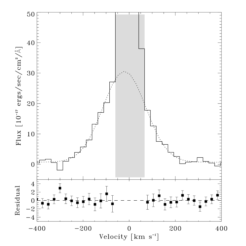
Figure 3: The profile of the [N II] $\lambda$6583 Spot 1 emission obtained with the G750M (6581) grating in 1999 August. The low-velocity region (shaded) was dominated by emission from the circumstellar ring and was excluded from the fit. The best-fit Gaussian (dotted) to the Spot 1 emission is shown. The velocity scale has been corrected for the heliocentric velocity of the LMC ($285\rm~{}km~{}s^{-1}$). The residual to the best-fit Gaussian is also shown.

Figure 4: (a) The interstellar absorption correction factors for emission lines C II $\lambda\lambda$1335,1336 (dot-dash), Si IV $\lambda\lambda$1394, 1403 (dash), C IV $\lambda\lambda$1548, 1551 (dot), and Mg II $\lambda\lambda$2796, 2803 (solid). The peak velocity, $V_{0}$, of the model Spot 1 emission is assumed to be $-30\rm~{}km~{}s^{-1}$. (b) The correction factor for C IV $\lambda\lambda$1548, 1551 doublet is plotted against the FWHM velocity of the input model Spot 1 Gaussian profile with peak velocities $V_{0}=0\rm~{}km~{}s^{-1}$ (solid), $-25\rm~{}km~{}s^{-1}$ (dots), $-50\rm~{}km~{}s^{-1}$ (dash), $-75\rm~{}km~{}s^{-1}$ (dot-dash), and $-100\rm~{}km~{}s^{-1}$ (dot-dot-dot-dash).

2D cylindrically symmetric hydrodynamical simulations ($800\times 600$ zones) of a blast wave overtaking a dense obstacle with darker shade representing higher density. The left panels (Scenario 1) show the development of a shock ($V_{b}=2,000\rm~{}km~{}s^{-1}$, $\rho_{HII}=150\mbox{ amu cm}^{-3}$, $d_{spot}=4\times 10^{16}\mbox{ cm}$, $\rho_{0}=10^{4}\mbox{ amu cm}^{-3}$) where the cooling time is comparable to the time for the fast shock to cross the obstacle, i.e., $t_{cool}\approx t_{cross}$. Shocks that have undergone radiative collapse and developed dense post-shock layers (R), and shock that remained non-radiative (NR), are indicated. The right panels (Scenario 2) show the development of a shock ($V_{b}=3,500\rm~{}km~{}s^{-1}$, $\rho_{HII}=150\mbox{ amu cm}^{-3}$, $d_{spot}\approx 4\times 10^{16}\mbox{ cm}$, $\rho_{0}=10^{5}\mbox{ amu cm}^{-3}$) where $t_{cool}\ll t_{cross}$. Due to the high density in this obstacle, all of the transmitted shocks undergo thermal collapse almost immediately.

The pressure behind the reflected shock as a function of obliquity immediately after impact of the blast wave for a spherical cloud having a density enhancement $\delta=\rho_{0}/\rho_{HII}\approx 70$. We do not show the function for obliquities higher than $135^{\circ}$ since the behavior at the back of a cloud is complex and highly time dependent due to the “healing” of the blast wave.

Range of transmitted shock velocities ($V_{shock}$) as a function of pre-shock density ($\rho_{0}$) for three different estimates of the blast-wave pressure. The shaded grey region shows the range of transmitted shock velocities (due to obliquity) for our best estimate of the blast-wave pressure ($V_{b}=3500\rm~{}km~{}s^{-1}$, $\rho_{HII}=150\mbox{ amu cm}^{-3}$). The upper boundary is the velocity of the transmitted shock at the tip of the protrusion and the lower boundary is the velocity at the side of the protrusion. The range of allowed shock velocities for our high blast-wave pressure estimate [$V_{b}=4100\rm~{}km~{}s^{-1}$, $\rho_{HII}=250\mbox{ amu cm}^{-3}$ (dashed)], and the low estimate [$V_{b}=2800\rm~{}km~{}s^{-1}$, $\rho_{HII}=100\mbox{ amu cm}^{-3}$ (dotted)] are also shown.

The top figure shows the temperature (thin) and density (thick) structure for electrons (dashed) and protons (solid) in a radiative shock of velocity $V_{s}=250\rm~{}km~{}s^{-1}$. The bottom figure shows the integrated line emissivities for N V $\lambda$1240 (dotted), C IV $\lambda$1550 (long dashes), [N II] $\lambda\lambda$6548, 6584 (short dashes), and ${\rm H}\alpha$ (solid). The shading identifies the different regions of the shock as described in the text.

Model shock cooling time $t_{cool}$ versus shock velocity $V_{shock}$ for initial obstacle density $\rho_{0}=2\times 10^{4}\mbox{ amu cm}^{-3}$ (solid). The power-law fit $t_{cool}\propto V_{s}^{3.8}$ (dashed) is also shown.

Line production efficiencies $\eta$ for N V $\lambda$1240 (dotted), C IV $\lambda$1550 (long dashes), [N II] $\lambda\lambda$6548, 6584 (short dashes), and ${\rm H}\alpha$ (solid) as a function of shock velocity for fully cooled shocks (thick) and shocks which have only aged for 3 years (thin).

Similar to Figure Modelling the Hubble Space Telescope Ultraviolet and Optical Spectrum of Spot 1 on the Circumstellar Ring of SN 1987A , with additional lines (thick) dividing the phase space between radiative shocks and non-radiative shocks for cooling time $t_{cool}=$ 2 and 4 years.

Contours of equal line ratios for [O I] (6300+6364)/5577 = $18.5\pm 4.2$ (long dash), [O III] (4959+5007)/4363 = $6.6\pm 3.4$ (short dash), [N II] (6548+6584)/5755 = $2.0\pm 0.2$ (dot dash), [S II] (6717+6731)/(4068+4076) = $0.1\pm 0.04$ (dotted), and [S III] (9068+9530)/6312 = $20.7\pm 10.9$ (solid). The middle line corresponds to the determined ratio of the dereddened line fluxes while the other two curves bracket the 1$\sigma$ errors. Since the [O III] $\lambda$4363 line may be blended with some Fe emission, the measured ratio is a lower limit. The arrow attached to the [O III] ratio contours shows how this may affect the derived temperature and density.

The observed (error bars) and modelled (Model 1: empty squares; Model 2: filled circles) light curves for the UV lines. The dashed line shows the earliest date (day 2932) that Spot 1 appeared as reported by Lawrence et al. (2000a).

Shock area growth for the $V_{s}=135\rm~{}km~{}s^{-1}$ (filled sqaures) and $V_{s}=250\rm~{}km~{}s^{-1}$ (empty circles) shocks in the best-fit Model 2 scenario. The dashed line shows the earliest date (day 2932) that Spot 1 appeared as reported by Lawrence et al. (2000a).

Model shock-front geometries and flow fields for the radiative shocks in the obstacle (shock incident from the left side). The shock speed varies along the surface from $250\rm~{}km~{}s^{-1}$ at the front to $100\rm~{}km~{}s^{-1}$ at the back. Cylindrical symmetry is assumed for all models.

Model ${\rm H}\alpha$ line profiles (solid) for the shock-front geometries in Figure Modelling the Hubble Space Telescope Ultraviolet and Optical Spectrum of Spot 1 on the Circumstellar Ring of SN 1987A are shown. These profiles are smoothed with a Gaussian with FHWM $=100\rm~{}km~{}s^{-1}$ (dotted). The day 4568 ${\rm H}\alpha$ line profile from the medium resolution 0$\farcs$1 G750M data is plotted for comparison (square). The uncertainties of the observed profile are smaller than the size of the symbol. The low-velocity region ($-50$ to $+50\rm~{}km~{}s^{-1}$) is dominated by emission from the circumstellar ring (cf. Figure 3) and is therefore not displayed.

One-dimensional VH-1 simulation (800 spatial zones) of a radiative shock ($V_{s}\approx 250\rm~{}km~{}s^{-1}$) developing in a dense ($n_{0}=3.3\times 10^{4}\mbox{ cm}^{-3}$) obstacle. Shown is a space-time diagram where darker shade represents higher density. The overall flow is advecting to the left due to the inflow boundary conditions chosen for the right-side boundary ($V_{inflow}=220\rm~{}km~{}s^{-1}$).

Two-dimensional VH-1 simulation ($80\times 400$ zones) of the development of a “turbulent” cold layer behind a radiative shock ($V_{s}\approx 250\rm~{}km~{}s^{-1}$) in a dense ($n_{0}\approx 3.3\times 10^{4}\mbox{ cm}^{-3}$) obstacle. The elapsed time between individual frames is one year. The obstacle has an imposed 5% sinusoidal density perturbation in a direction perpendicular to the shock front.

References

- Baron et al. (2000) Baron, E., et al. 2000, ApJ, 545, 444
- Beuermann et al. (1994) Beuermann, K., Brandt, S., & Pietsch, W. 1994, A&A, 281, L45
- Bionta et al. (1987) Bionta, R. M., et al. 1987, Phys. Rev. Lett., 58, 1494
- Blades et al. (1988) Blades, J. C., Wheatley, J. M., Panagia, N., Grewing, M., Pettini, M., & Wamsteker, W. 1988, ApJ, 334, 308
- Blinnikov et al. (2000) Blinnikov, S., Lundqvist, P., Bartunov, O., Nomoto, K., & Imamoto, K. 2000, ApJ, 532, 1132
- Blondin & Lundqvist (1993) Blondin, J. M., & Lundqvist, P. 1993, ApJ, 405, 337
- Böhm & Goodson (1997) Böhm, K.-H., & Goodson, A. 1997, in IAU Symp. 182, Herbig-Haro Flows and the Birth of Low Mass Stars, ed. B. Reipurth & C. Bertout (Dordrecht: Kluwer), 47
- Borkowski et al. (1997a) Borkowski, K., Blondin, J., & McCray, R. 1997a, ApJ, 476, L31
- Borkowski et al. (1997b) ———. 1997b, ApJ, 477, 281
- Burrows et al. (1995) Burrows, C. J., et al. 1995, ApJ, 454, 680
- Burrows et al. (2000) Burrows, D. N., et al. 2000, ApJ, 543, L149
- Cargill & Papadopoulos (1988) Cargill, P. J., & Papadopoulos, K. 1988, ApJ, 329, L29
- Cardelli et al. (1989) Cardelli, J. A., Clayton, G. C., & Mathis, J. S. 1989, ApJ, 345, 245
- Colella & Woodward (1984) Colella, R., & Woodward, P. R. 1984, J. Comp. Phys., 54, 174
- Cox & Raymond (1985) Cox, D. P., & Raymond, J. C. 1985, ApJ, 298, 651
- Chevalier & Dwarkadas (1995) Chevalier, R. A., & Dwarkadas, V. V. 1995, ApJ, 452, L45
- Chevalier & Imamura (1982) Chevalier, R. A, & Imamura, J. N. 1982, ApJ, 261, 543
- Chugai et al. (1997) Chugai, N. N., Chevalier, R. A., Kirshner, R. P., & Challis, P. M. 1997, ApJ, 483, 925
- Crotts & Heathcote (2000) Crotts, A. & Heathcote, S. 2000, ApJ, 528, 426
- Cumming & Lundqvist (1997) Cumming, R. J., & Lundqvist, P. 1997, in Advances in Stellar Evolution, ed. R. T. Rood (Cambridge: CUP), 297
- Ensman & Burrows (1992) Ensman, L., & Burrows, A. 1992, ApJ, 393, 742
- Fitzpatrick (1986) Fitzpatrick, E. L. 1986, AJ, 92, 1068
- Fitzpatrick (1999) ———. 1999, PASP, 111, 63
- Fitzpatrick & Walborn (1990) Fitzpatrick, E. L., & Walborn, N. R. 1990, AJ, 99, 1483
- Fransson et al. (1989) Fransson, C., Cassatella, A., Gilmozzi, R., Kirshner, R. P., Panagia, N., Sonneborn, G., & Wamsteker, W. 1989, ApJ, 336, 429
- Gaensler et al. (1997) Gaensler, B. M., Manchester, R. N., Staveley-Smith, L., Tzioumis, A. K., Reynolds, J. E., & Kesteven, M. J. 1997, ApJ, 479, 845
- Garnavich et al. (1997) Garnavich, P., Kirshner, R., & Challis, P., 1997, IAU Circ. 6710
- Garnavich et al. (2000) Garnavich, P., Jha, S., Challis, P., & Kirshner, R. 2000, IAU Circ. 7360
- Garnavich et al. (2001) Garnavich, P., et al. 2001, ApJL, submitted
- Gorenstein et al. (1994) Gorenstein, P., Hughes, J. P., & Tucker, W. H. 1994, ApJ, 420, L25
- Hasinger et al. (1996) Hasinger, G., Aschenbach, B., & Trümper, J. 1996, A&A, 312, L9
- Hester et al. (1986) Hester, J. J., Danielson, G. E., & Raymond, J. C. 1986, ApJ, 303, L17
- Hirata et al. (1987) Hirata, R., et al. 1987, Phys. Rev. Lett., 58, 1490
- Imamura et al. (1984) Imamura, J. N., Wolff, M. T., & Durisen, R. H. 1984, ApJ, 276, 667
- Innes et al. (1987) Innes, D. E., Giddings, J. R., & Falle, A. E. G. 1987, MNRAS, 226, 67
- Innes (1992) Innes, D. E. 1992, A&A, 256, 660
- Jakobsen et al. (1991) Jakobsen, P., et al. 1991, ApJ, 369, L63
- Kirshner et al. (1987) Kirshner, R. P., Sonneborn, G., Crenshaw, D. M., & Nassiopoulos, G. E. 1987, ApJ, 320, 602
- Lawrence et al. (2000a) Lawrence, S. S., Sugerman, B. E., Bouchet, P., Crotts, A. P. S., Uglesich, R., & Heathcote, S. 2000a, ApJ, 537, L123
- Lawrence et al. (2000b) Lawrence, S. S., Sugerman, B. E., & Crotts, A. P. S. 2000b, IAU Circ. 7419
- Leitherer et al. (2000) Leitherer, C., et al. 2000, “STIS Instrument Handbook,” Version 4.0, (Baltimore: STScI), 343
- Lentz et al. (2001) Lentz, E. J., et al. 2001, ApJ, 547, 406
- Link et al. (2001) Link, R., Rosenberg, D. L., & Chevalier, R. A. 2001, in Interacting Winds from Massive Stars, A.S.P. Conference Series (San Francisco: ASP), in press (astro-ph/0107127)
- Long & Blair (1990) Long, K. S., & Blair, W. P. 1990, ApJ, 358, L13
- Lundqvist (1999) Lundqvist, P. 1999, ApJ, 511, 389
- Lundqvist & Fransson (1991) Lundqvist, P., & Fransson, C. 1991, ApJ, 380, 575
- Lundqvist & Fransson (1996) ———. 1996, ApJ, 464, 924
- Lundqvist & Sonneborn (2001) Lundqvist, P., & Sonneborn, G. 2001, in SN 1987A: Ten Years After, eds. M. Phillips & N. Suntzeff, A.S.P. Conference Series (San Francisco: ASP), in press (astro-ph/9707144)
- Luo & McCray (1991) Luo, D., & McCray, R. 1991, ApJ, 379, 659
- Luo et al. (1994) Luo, D., McCray, R., & Slavin, J. 1994, ApJ, 430, 264
- Manchester et al. (2001) Manchester, R. N., Gaensler, B., M., Wheaton, V. C., Staveley-Smith, L., Tzioumis, A. K., Bizunok, N. S., Kesteven, M. J., Reynolds, J. E. 2001, Proc. Astro. Soc. Australia, accepted (astro-ph/0110693)
- Maran et al. (2000) Maran, S. P., Sonneborn, G., Pun, C. S. J., Lundqvist, P., Iping, R., & Gull, T. R. 2000, ApJ, 545, 390
- Martin & Arnett (1995) Martin, C., & Arnett, W. D. 1995, 447, 378
- Masai & Nomoto (1994) Masai, K., & Nomoto, K. 1994, ApJ, 424, 924
- Michael et al. (1998a) Michael, E., McCray, R., Borkowski, K. J., Pun, C. S. J., & Sonneborn, G. 1998a, ApJ, 492, L143
- Michael et al. (1998b) Michael, E., et al. 1998b, ApJ, 509, L117
- Michael et al. (2000) ———. 2000, ApJ, 542, L53
- Osterbrock (1989) Osterbrock, D. E. 1989, Astrophysics of Gaseous Nebulae and Active Galactic Nuclei. (Mill Valley: University Science Books)
- Panagia et al. (2000) Panagia, N., Romaniello, M., Scuderi, S., & Kirshner, R. P. 2000, ApJ, 539, 197
- Park et al. (2001) Park, S., Burrows, D. N., Garmire, G. P., Nousek, J. A., McCray, R., Michael, E., & Zhekov, S. 2001, ApJ, accepted (astro-ph/0111116)
- Plait et al. (1995) Plait, P. C., Lundqvist, P., Chevalier, R. A., & Kirshner, R. P. 1995, ApJ, 439, 730
- Pun et al. (1995) Pun, C. S. J., et al. 1995, ApJS, 99, 223
- Ramsbottom et al. (1994) Ramsbottom, C.A., Berrington, K.A., Hibbert, A., & Bell, K.L. 1994, Phys. Scripta, 50, 246
- Raymond (1979) Raymond, J. C. 1979, ApJS, 39, 1
- Russell & Dopita (1992) Russell, S. C., & Dopita, M. A. 1992, ApJ, 384, 508
- Scuderi et al. (1996) Scuderi, S., Panagia, N., Gilmozzi, R., Challis, P. M., & Kirshner, R. P., 1996, ApJ, 465, 956
- Seaton (1979) Seaton, M. J. 1979, MNRAS, 187, 73P
- Sgro (1975) Sgro, A. G. 1975, ApJ, 197, 621
- Sonneborn et al. (1997) Sonneborn, G., et al. 1997, ApJ, 477, 848
- Sonneborn et al. (1998) Sonneborn, G., et al. 1998, ApJ, 492, L139
- Staveley-Smith et al. (1992) Staveley-Smith, L., et al. 1992, Nature, 355, 147
- Staveley-Smith et al. (1993) Staveley-Smith, L., Briggs, D. S., Rowe, A. C. H., Manchester, R. N., Reynolds, J. E., Tzioumis, A. K., & Kesteven, M. J. 1993, Nature, 366, 136
- Strickland & Blondin (1995) Strickland, R., & Blondin, J. M. 1995, ApJ, 449, 727
- Suzuki et al. (1993) Suzuki, T., Shigeyama, T., & Nomoto, K. 1993, A&A, 274, 883
- Tielens et al. (1994) Tielens, A. G. G. M., McKee, C. F., Seab, C. G. & Hollenbach, D. J. 1994, ApJ, 431, 321
- Walborn et al. (1993) Walborn, N. R., Phillips, M. M., Walker, A. R., & Elias, J. H. 1993, PASP, 103, 1240
- Walder & Folini (1998) Walder, R., & Folini, D. 1998, A&A, 330, L21
- Walker & Suntzeff (1990) Walker, A. R., Suntzeff, N. B. 1990, PASP, 102, 131
- Wampler et al. (1989) Wampler, E. J., Richichi, A., & Baade, D. 1989, in IAU Colloq. 120, Structure and Dynamics of the Interstellar Medium, ed. G. Tenorio-Tagle, M. Modes, & J. Melnick (Berlin: Springer), 190
- Wang (1991) Wang, L. 1991, A&A, 246, L69
- Wang et al. (1996) Wang, L., et al. 1996, ApJ, 466, 998
- Welty et al. (1999) Welty, D. E., Frisch, P. C., Sonneborn, G., & York, D. G. 1999, ApJ, 512, 636
- Zeldovich & Raizer (1967) Zeldovich, Ya. B., & Raizer, Yu. P. 1967, Physics of Shock Waves and High-Temperature Hydrodynamic Phenomena (New York: Academic Press)