Luminous infrared galaxies as possible sources of the UHE cosmic rays

Abstract

Ultra High Energy (UHE) particles coming from discrete extragalactic sources are potential candidates for EAS events above a few tens of EeV. In particular, galaxies with huge infrared luminosity triggered by collision and merging processes are possible sites of UHECR acceleration. Here we check whether this could be the case. Using the PSCz catalogue of IR galaxies we calculate a large scale anisotropy of UHE protons originating in the population of the luminous infrared galaxies (LIRGs). Small angle particle scattering in weak irregular extragalactic magnetic fields as well as deflection by regular Galactic field are taken into account. We give analytical formulae for deflection angles with included energy losses on cosmic microwave background (CMB). The hypotheses of the anisotropic and isotropic distributions of the experimental data above 40 EeV from AGASA are checked, using various statistical tests. The tests applied for the large scale data distribution are not conclusive in distinguishing between isotropy and our origin scenario for the available small data sample. However, we show that on the basis of the small scale clustering analysis there is a much better correlation of the UHECRs data below GZK cut-off with the predictions of the LIRG origin than with those of isotropy. We derive analytical formulae for a probability of a given number of doublets, triplets and quadruplets for any density distribution of independent events on the sky. The famous AGASA UHE triple event is found to be very well correlated on the sky with the brightest extragalactic infrared source within 70 Mpc - merger galaxies Arp 299 (NGC 3690 + IC 694).

1 Introduction

The existence of the UHE cosmic rays, after their discovery almost half a century ago, remains still puzzling. In advent of the new giant experiment named in honour of Pierre Auger, there are many proposals to explain their origin. UHE cosmic rays (UHECR) seem to be extragalactic because their arrival directions are not correlated with the Galactic disk. Thus, sites of their origin should be different from normal galaxies (like our Galaxy). In this work we check the hypothesis that the powerful luminous infrared galaxies (LIRGs) might be the UHECR sources. Large fraction of bright IR galaxies are found to be interacting systems, suggesting that collision and merging processes are mostly responsible in triggering the huge IR light emission [19]. Fraction of interacting systems increases with IR luminosity and in the population of the most IR luminous objects in the Universe almost all appear as gravitationally interacting. Favourable environments for accelerating particles to UHE regime via the first order Fermi process are provided by amplified magnetic fields on the scale of tens kpc resulting from gravitational compression, as well as high relative velocities of galaxies and/or superwinds from multiple supernovae explosions [4, 5]. There have been several observational claims that colliding galaxies could be possible sites of the UHECR origin. Al-Dargazelli et al[2] have proposed that some clustering of UHECR shower directions above 10 EeV are associated with nearby colliding galaxies. Uchihori et al[27] have analysed combined world data from Northern hemisphere experiments and concluded that two triplets and a doublet lie in a vicinity of interacting systems. Takeda et al[25] have noticed that the interacting galaxy VV 141 at z=0.02 is a possible candidate for the triplet of events above 50 EeV from the AGASA experiment. However, as we shall show, there is another favourable candidate for the origin of this UHECR cluster - Arp 299 (Mrk171, VV 118a/b), a member of LIRG class of extragalactic objects. This system (RA$=171.4^{\circ}$, $\delta=58.8^{\circ}$), consisting of two interacting starburst galaxies, is the closest extragalactic object (distance 42 Mpc for $H_{0}=75km\,s^{-1}\,Mpc^{-1}$) with IR luminosity greater than $5\times 10^{11}L\odot$ ($\simeq 2\times 10^{45}ergs\,s^{-1}$) and it is the brightest IR source within 70 Mpc. Such high IR luminosity is related to young and violent star forming regions. There is also observational evidence of superwind outflows, large scale strong radio emissions and the estimated supernova rate is about 0.6 per year [1, 13, 14, 21].
The aim of the present paper is to check whether the LIRGs could be the sites of origin of the UHECRs observed at the Earth. Using the PSCz catalogue [20] we construct the all-sky maps of UHE proton intensities originating in LIRGs, taking into account effects of particle propagation through the extragalactic medium and, as an example, possible influence of the regular galactic magnetic field (GMF). We check both hypotheses: origin in LIRGs and, on the other hand, the isotropic distribution of the experimental data above 40 EeV from AGASA [12], using various statistical tests.

2 Anisotropy calculations

2.1 The PSCz catalogue

The PSCz catalogue consists of almost 15000 IR galaxies with known redshifts, covering 84% of the sky. It should be noted that observational limitations cause that some of the extragalactic objects may not have measured redshifts or may be even unobserved in the dust obscured regions within the disk of the Galaxy (the so called zone of avoidance). Figure 1 (top) presents the distribution of all PSCz galaxies with known redshifts. We can see patches on the sky regions excluded from the catalogue. On inspection of the superimposed directions of the AGASA showers above 40 EeV we can find only a few cases where experimental events lie in the vicinity of excluded regions, which should not affect much our analysis. As the potential UHECR sources we have selected objects with luminosities in the far infrared (FIR) range exceeding LIRG limit $L_{FIR}=10^{11}L_{\odot}$, that is over one order of magnitude greater than the estimated FIR luminosity of our Galaxy [7], and with distances up to 1 Gpc, giving the total number of 2811 sources (figure 1, bottom). A large fraction of such objects show to be in an apparent stage of collision and merging.

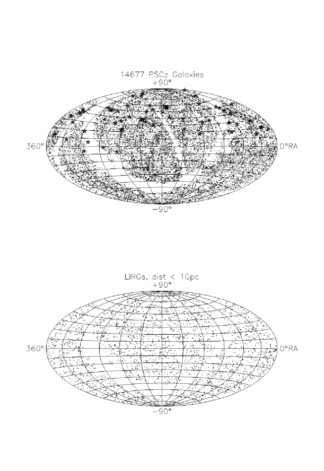
Figure 1: Top: Sky distribution of 14677 PSCz galaxies with known redshifts and superimposed AGASA showers above 40 EeV (stars). Aitoff projection in equatorial coordinates. Bottom: Selected 2811 objects with $L_{FIR}>10^{11}L_{\odot}$ and with distances up to 1 Gpc

2.2 CR propagation

To predict the CR anisotropy expected in the model of LIRG origin we have assumed the following:

• Protons are injected at the sources with a spectrum $dN/dE\sim E^{-2}$ truncated at $10^{21}$ eV.

• CR luminosity at the source is proportional to its $L_{FIR}$ luminosity.

• CR propagate through the intergalactic medium, where they are scattered and suffer energy losses on the cosmic microwave background (CMB)[3].

To calculate CR arrival directions we have derived an analytical formula for the distribution of the deflection angles, for the multiple small angle scattering in weak irregular magnetic fields with continuous energy losses taken into account (see Appendix A). Since strength and structure of the extragalactic magnetic field are largely unknown, we adopt here the upper limit for this field magnitude and coherence scale: $B\,(l_{c})^{1/2}=1\,nG\,(1Mpc)^{1/2}$, as measured by Faraday rotation of radio signals from distant quasars [15]. Because the analysis is strongly energy dependent, we consider two energy regions 40 to 80 EeV and above 80 EeV, where this limit is just about the Greisen-Zatsepin-Kuzmin (GZK) flux cut-off predicted from CR interactions with the 2.7 K CMB radiation [10, 30].

2.3 Maps of the expected anisotropy

Equatorial maps of the expected intensity of the UHE protons originating in LIRGs for two energy regions, 40-80 EeV and above 80 EeV, with sky coverage and declination dependent exposure for the AGASA experiment [25] (see also Appendix B), are presented in figures 2 (top) and 3 with superimposed AGASA events.

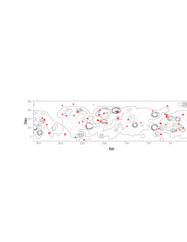
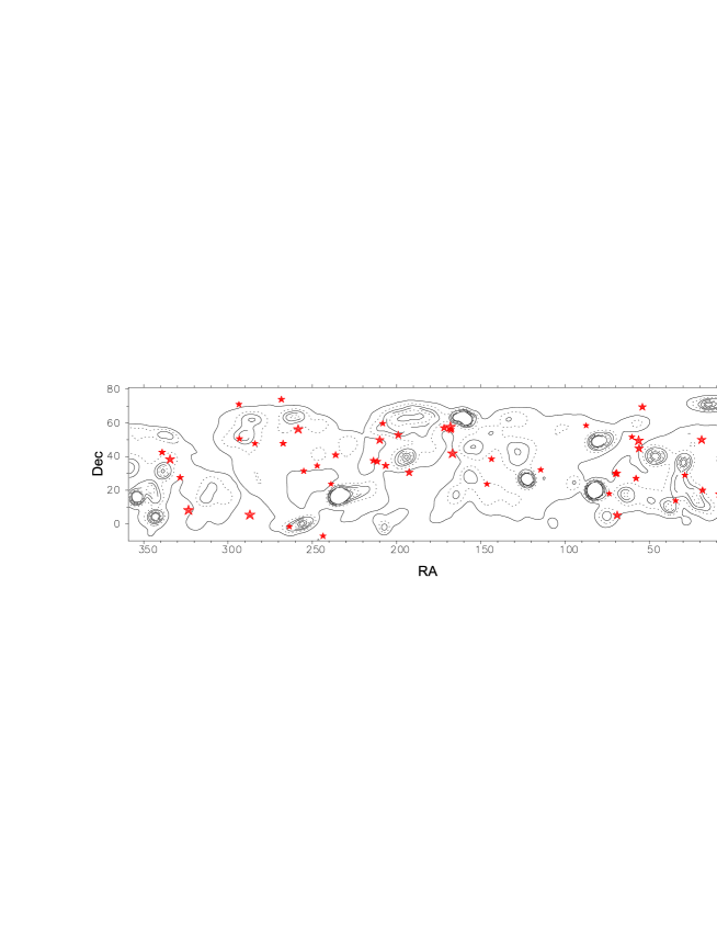
Figure 2: Expected maps of proton intensities without (top) and with (bottom) influence of the regular galactic magnetic field (model BSS-A) for protons with 40-80 EeV originating in LIRGs to be seen by AGASA, with superimposed 47 AGASA shower directions in this energy range (stars scaled with energy). Contours of constant flux per unit solid angle are spaced linearly.

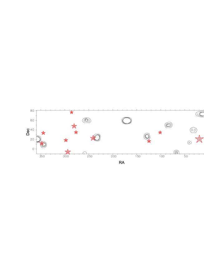
Figure 3: Expected map of proton intensities (energy above 80 EeV) from LIRGs to be seen by AGASA, with superimposed 11 AGASA showers in this energy range (no GMF).

In figure 2 (top) we can see that expected proton intensities for 40-80 EeV show good correlation with the distribution of the experimental events from AGASA. Especially, clearly visible is the region of the sky where high proton intensities from Arp 299 correlate with the AGASA triplet of events (RA$\approx 170^{\circ}$, $\delta\approx 60^{\circ}$). At higher energies, because of the rapid proton energy losses on CMB, only sources located at distances not larger than 100 Mpc are visible on the map. No correlation of the data events above 80 EeV with the expected CR intensities can be seen (figure 3). There is an apparent group of UHE showers in the region with RA$\approx 300^{\circ}$, where no possible sources exist. However some of the showers from this group lie close to the region heavily obscured by the Galactic disk.

2.4 Influence of Galactic magnetic field

The global regular GMF structure is not well known. Analyses of rotation measures of pulsars and extragalactic radio sources suggest that the GMF has a bisymmetric spiral (BSS) form with field directions reversed from arm to arm [22, 11]. This is also supported by the observed value of the pitch angle of the local field and number of field reversals within the Galactic disk [6, 11, 18]. To examine the influence of the regular GMF on the extragalactic UHE fluxes we have chosen the bisymmetric spiral model with field reversals and odd parity (BSS-A) adopted from Stanev [24]. Because the predictions are strongly model dependent, and the procedure applied gives a rather simplified picture, the analysis presented here is only an example of the possible extragalactic CR flux distortion. It is presented for the lower energy range 40-80 EeV, where the effect is stronger and easily visible.
Simulations of a large number of monoenergetic antiprotons ejected from the Earth and followed to the halo border through GMF give flux modification factors depending on directions in the ’extragalactic’ sky. Then, for an assumed flux distribution of protons at the Galactic borders we are able to calculate their fluxes at the Earth. Distortion effects i.e. reduction or magnification and shifting of the particle fluxes are visible in Figure 2 (bottom). The modification of the extragalactic UHECR intensities due to the influence of the GMF BSS-A model seems to worsen the correlation with the experimental data seen in the upper figure.

3 Statistical tests and results

3.1 Smirnov-Cramer-von Mises test

To check the hypotheses of isotropic and anisotropic distribution of the experimental data above 40 EeV from AGASA, we have used Smirnov-Cramer-von Mises (SCvM) free of binning test [8], modified for a 2-dimensional distribution analysis. SCvM test is based on comparing the cumulative distribution function $F(X)$ under hypothesis $H_{0}$ with the equivalent function $S_{N}(X)$ of the data. The considered statistics $W^{2}$ is defined as follows

$$W^{2}=\int_{-\infty}^{\infty}\Big{(}S_{N}(X)-F(X)\Big{)}^{2}f(X)dX$$ (1)

where $f(X)$ is the probability density function corresponding to the hypothesis $H_{0}$. $S_{N}(X)$ is based on the experimental data (two coordinates of the UHECR events on the equatorial map) and always increases in steps of equal height, $N^{-1}$, where $N$ is the total number of data. It is worth to note that this test is reliable even for small statistics ($N\geq 3$). Critical $NW^{2}$ values for the confidence level $\alpha=$0.1 and 0.05 are 0.347 and 0.461 respectively.

• E	Tested hypotheses	NW2 values
  40-	Isotropy	0.063; 0.116; 0.202; 0.263
  80	LIRGs anisotropy	0.069; 0.121; 0.106; 0.215
  EeV	LIRGs anisotropy + GMF	0.115; 0.195; 0.181; 0.247
  $>$80	Isotropy	0.042; 0.573; 0.658; 0.071
  EeV	LIRGs anisotropy	0.631; 0.351; 2.177; 0.338

Table 1:

Each of the cumulative distribution functions, $F(X)$ and $S_{N}(X)$, is the integral of the probability density function over the rectangle area defined by the coordinate point and one of the corners of the map. In this way, from the 2-dimensional maps we have constructed a 1-dimensional $F(X)$ and $S_{N}(X)$, for four cases depending on the chosen corner of the map. Although the four obtained $NW^{2}$ values are not completely independent, they provide a valuable insight into the analysis. Results of tested hypotheses: isotropy and LIRGs anisotropy (with and without GMF), energies 40-80 EeV and above 80 EeV are shown in table 1. All the hypotheses in the energy range 40-80 EeV pass, assuming confidence level $\alpha=$0.1 ($NW^{2}$=0.347). However, with the presence of the GMF the agreement is worse. The hypotheses for energies above 80 EeV fail, especially in LIRG anisotropy scenario.
Irrespective of the above, table 1 shows that it is not easy to draw conclusions from this test as the $NW^{2}$ values calculated for different map corners scatter quite significantly. Thus, it is advisable to apply another, hopefully more powerful, statistical test

3.2 Eigenvector test

The idea is based on assigning unit directional vectors to the data points on the celestial sphere. By finding the normalized eigenvalues $\tau_{1}$, $\tau_{2}$, $\tau_{3}$ of the orientation matrix $\mathbf{T}$ constructed for the N unit data vectors it is possible to discriminate between the isotropic and some anisotropic distributions [9]. Assuming $0\leq\tau_{1}\leq\tau_{2}\leq\tau_{3}\leq 1$ the empirical shape criterion $\gamma=$ $\left[log_{10}(\tau_{3}/\tau_{2})\right]/\left[log_{10}(\tau_{2}/\tau_{1})\right]$, and the strength parameter $\zeta=log_{10}(\tau_{3}/\tau_{1})$ are used to discriminate girdle type from clustered distribution. Distributions of the girdle and cluster type plot with $\gamma$ below and above unity, respectively. Intermediate i.e. partly girdle, partly cluster distributions plot around the line $\gamma=1$. Isotropic distributions plot with strength $\zeta$ near zero.
In figure 4 (left) there are shown distributions of 500 samples, consisting of 47 events each, simulated under isotropic (dots) and LIRGs anisotropic (crosses) scenarios.

Figure 4: Left: Eigenvalue analysis distributions (each point corresponds to 47 events) drawn from isotropy (dots) and LIRGs anisotropy (crosses) scenarios. Points based on AGASA data (star and thick cross represents respectively our and Medina Tanco calculation from ’old’ AGASA data - 47 events with energy above 40 EeV. The open square is for ’new’ data - 47 events, 40-80 EeV); Right: Simulations, as previously, but for large samples of 500 events each.

The open square denotes AGASA data, 47 events with energy 40-80 EeV. The two hypotheses, LIRG anisotropy and isotropy, correspond to the two regions in the $\zeta-\gamma$ plane which overlap significantly for the 47 event samples. Mostly due to the small statistics considered, the eigenvector analysis is not sensitive enough to distinguish between isotropic and LIRG anisotropic origin of the experimental data. Hopefully with a sample of more than 500 events, to be collected in a few months of a full operational mode of the Auger observatory, the two distributions should separate (figure 4, right).
The eigenvector method has been already applied to the UHECR anisotropy analysis by Medina Tanco [17]. The point corresponding to the ’old’ AGASA data (47 events above 40 EeV), calculated by this author, is shown on the $\zeta-\gamma$ plane (thick cross in figure 4, left) lying well away from the simulated isotropic distribution. However, the point calculated by us for the same AGASA data (star) has a lower strength value and lies on the isotropy distribution. Thus, contrary to the result of Medina Tanco, the AGASA data do not show such a strong clustering (on the basis of the eigenvector analysis) to differ from the isotropy distribution. We have checked the correctness of our result by calculating the eigenvalues of the orientation matrix also analytically (which is possible for a 3x3 matrix).
We have not done the eigenvector analysis for the data above 80 EeV because of the sample of 11 events was too small.

Figure 5: Probability distributions of doublets for isotropic (circles) and LIRGs anisotropic (crosses) scenarios for the cases of zero (solid line) and one triplet (dashed line).

3.3 Multiplet analysis

Apart from analysing the large scale LIRG anisotropy (as in previous chapters) we will check this hypothesis by analysing probabilities of multiplets, i.e. groups of events with small angular separation.
In the available AGASA data from 40-80 EeV there are two doublets (separation angles smaller than 2.5^∘) and one triplet (with criteria taken from the AGASA publication [25], see also Appendix B). Figure 5 shows probability distribution of the number of doublets based on the $10^{4}$ samples of 47 events each, simulated from the LIRGs anisotropic map (crosses) for the cases of zero and one triplet. There are also similar probabilities for the isotropy scenario (circles), calculated analytically (Appendix B). From figure 5 we find that the probability of obtaining at least the observed number of multiplets from LIRGs anisotropy scenario is $0.129$ ($7.1\times 10^{-2}$) for more than two (three) doublets, while from isotropy (with the same assumed response in declination of the AGASA experiment) it is only $0.67\times 10^{-2}\,(0.2\times 10^{-2}$). All AGASA events above 40 EeV have one triplet and six doublets, a collection even less probable to be obtained from isotropy.
The above analysis may indicate only that there is some anisotropy (which increases mainly the probability of triplet) but not necessarily that correlated with LIRGs.

Figure 6: Smoothed cos($\theta$) distributions for separation angles between AGASA data (47 events 40-80 EeV) and 5000 events drawn from isotropic (dotted line) and LIRG anisotropic (solid line) distributions. Dashed line represents distribution of cosines within simulated LIRG events (47$\times$5000) averaged over $10^{3}$ samplings.

A relationship between the set of the data and our hypothesis can be checked by looking for small angle correlation between the simulated and the real events. In figure 6 there are shown smoothed distributions of $cos\theta$ in the range $0.9-1$, where $\theta$’s are separation angles between the AGASA events, from one side (47 events, 40-80 EeV) and, from another side, 5000 events drawn from the isotropic (dotted line) or from the LIRG (solid line) distributions (giving 47$\times$5000 cosine values for each case). The obvious flat distribution of $cos\theta$ between the AGASA data and isotropic events (dotted line) with a small rise from left to right shows the effect of the AGASA declination efficiency. The dashed line represents $cos\theta$ distribution for $\theta$ taken between the events simulated from the LIRG map (47$\times$5000 events), averaged over $10^{3}$ such runs. Here, a significant rise in the range of a few degrees ($\theta<8$ deg, $cos\theta>0.99$) indicates a clustering of the simulated LIRG events. A similar rise is seen in the distribution of $cos\theta$ between AGASA data and events simulated from LIRG (solid line). Taking into consideration the sum of all cosines above 0.99, the resulting value lies within 1.67 $\sigma$ from the mean value obtained from the LIRG scenario, confirming quite a strong correlation between the real and simulated LIRG events.
In figure 7 there are presented distributions of 47 events from AGASA and equivalent samples of events simulated from the map in figure 2 (top). We have estimated that the probability of getting a doublet or a triplet in the vicinity of Arp 299 is about 0.5. We can see that samples of the 47 events simulated from LIRGs anisotropy scenario, show good resemblance to the experimental data distribution.

Figure 7: Sky distribution comparison of the 47 AGASA showers with energy 40-80 EeV (top left) and examples of three simulations from LIRG anisotropy map. Equatorial coordinates.

4 Astrophysical implications

The strongest evidence for UHECRs origin may come from the correlation between directions of the AGASA triplet of events with energies 53.5, 55.0 and 77.6 EeV and an energetic astrophysical source in the local Universe. So far Arp 299 is the best candidate as a member of LIRGs, the brightest infrared source within 70 Mpc and a system of colliding galaxies showing intense, violent starburst activity at only 42 Mpc away. It should be noted that Arp 299 appeared earlier as VV 118 in the list of candidates for the AGASA triplet presented by Takeda et al[25] but was not recognized as a colliding, energetic system, and, as a result, was not given enough attention. These authors point to another object VV 141 being a colliding system at z=0.02. However, as Arp 299 is at a distance two times smaller and fulfils the necessary criteria for CR acceleration, we think that it is this object which could be the most probable CR source.
Recent studies on the nature of LIRGs suggest that compact strong radio emission may result from frequent multiple luminous radio supernovae [21]. These objects are a poorly known class of supernovae with high nonthermal radio power indicating large kinetic energy input to accelerate particles [29]. In systems with intense starburst activity in extremely dense molecular gas and strong magnetic field environment, ”nearly every supernova explosion results in a luminous radio SN with very high radio power” [21]. It is also worth to note that there are some observations suggesting a relationship between gamma ray bursts (GRB) and supernovae explosions [16]. Very recently Weiler et al[28] have stated that GRB980425 and radio loud supernova SN1998bw are possibly related. Thus, it is not unreasonable to invoke here the intriguing hypothesis of the common origin of the two most energetic, mysterious phenomena in the Universe, UHECRs and GRBs.

5 Conclusions

We have shown that the available data from AGASA in the energy range 40 to 80 EeV are not in contradiction with the expected anisotropy of CR produced in LIRGs. After applying the GMF, the LIRG hypothesis passes as well, but an apparent worse agreement with the data, suggests that the GMF model used by us may not be appropriate. So, we may hope that, if point sources existed they would be useful for determining the global structure of the GMF. At energies above 80 EeV both the isotropic and the LIRGs anisotropic distribution hypotheses are rejected. This might be explained by an existence of a UHECR population of a different origin above GZK cut-off.
However, it seems that the SCvM test used here is not conclusive for distinguishing between the isotropy and the LIRGs distributions. Contrary to calculations done by other author, the eigenvector analysis has also appeared unable to do this for the existing sample sizes. Thus, we have considered a small scale clustering rather than a large scale anisotropy. Indeed, the analysis of multiplet probability gives good discrimination between isotropic and anisotropic scenarios (figure 5). The probability of the occurring of two doublets and one triplet (three doublets and one triplet) is 10 (20) times higher for the LIRG hypothesis than that for isotropy . The analysis of the distributions of the angular distances between the data and simulated LIRG events also supports an existence of a correlation (figure 6). The strongest argument for our hypothesis is the observation of the triplet from the direction of Arp299, a system of colliding galaxies. We have obtained, via simulations, a high probability of doublets and triplets from this source, estimated to be about 0.5.
Finally, with the prospect of new data to come from the Pierre Auger Observatory in a few years, the arrival direction distribution of UHECR should provide a much better clue to their origin.

Appendix A. Small angle scattering

Let us consider the statistical process of the small angle scattering of a charged particle on $N$ randomly oriented magnetic cells. Here we derive formulae for deviation angles and time delays on simple assumptions that statistical variables $\delta\vec{n}_{k}$ (denoting change of unit vector along direction of flight occurring in the $k$-th cell) are: 1) independent and small, 2) cumulative change of direction is also small, 3) the number of cells $N$ is large.

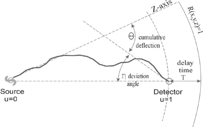
Figure 8: Schematic diagram of the particle trajectory through IGMF

As the particle energy changes along its trajectory, we have the relation

$$\langle\vec{\vartheta}_{k}^{2}\rangle=\langle\vec{\vartheta_{N}}^{2}\rangle\cdot\Bigg{(}\frac{E_{N}}{{E}_{k}}\Bigg{)}^{2}\equiv\langle\vec{\vartheta_{N}}^{2}\rangle\cdot\Bigg{(}\frac{E_{u=1}}{E_{u}}\Bigg{)}^{2}$$ (2)

Here $E_{N}$ and $E_{k}$ denote particle energies in $N^{th}$ and $k^{th}$ cells and $\langle\vec{\vartheta}_{N}^{2}\rangle$ is the mean square scattering angle in the last $N_{th}$ cell, which is at the detector. We also denote cells by a continuous variable $u=k/N$ instead of $k$ (i.e. $u=1$ indicates the detector). In this model the particle’s trajectory consists of $N$ segments of straight lines of equal length $L=1/N$. If the source of particles is placed in the centre of a sphere of radius $R=1$, then particle trajectories will end inside the sphere and the time delay is just the additional time the particle needs to reach the sphere. Looking back from the detector we miss the source by the deviation angle $\eta$ (figure A1). The formulae for the coordinates of the trajectory end: $x$,$y$, $z$ ($z$-axis is the particle initial direction), time delay $T$ and angle $\eta$ are shown below. The cumulative change of direction is described by the angle $\Theta_{k}$ as: $\vec{n_{k}}-\vec{n_{0}}=\sum_{i=1}^{k}\vec{\delta n_{i}}=\sum_{i=1}^{k}\vec{\vartheta_{i}}=\vec{\Theta_{k}}$.

$$x=\frac{1}{N}\cdot\sum_{k=1}^{N}\Theta_{xk};\quad y=\frac{1}{N}\cdot\sum_{k=1}^{N}\Theta_{yk};\quad$$ (3)

$$z=\frac{1}{N}\cdot\sum_{k=1}^{N}(1-\frac{1}{2}\Theta^{2}_{xk}-\frac{1}{2}\Theta^{2}_{yk});\quad\vec{\eta}=\sum_{k=1}{N}\frac{k}{N}\cdot\vec{\vartheta_{k}}$$

$$T\approx\Delta z-\frac{1}{2}\cdot(x^{2}+y^{2})\quad{}$$ (4)

$${}where\quad\Delta z=\frac{1}{N}\cdot\sum_{k=1}^{N}(\frac{1}{2}\Theta^{2}_{xk}+\frac{1}{2}\Theta^{2}_{yk})$$

We can calculate statistical moments for the above random variables. Here are some of them:

$$\langle\vec{\eta_{\,}}^{2}\rangle=N\cdot\langle\vec{\vartheta_{N}}^{2}\rangle\cdot f_{12};\quad\langle\vec{\eta}^{4}\rangle-\langle\vec{\eta}^{2}\rangle^{2}=\langle\vec{\eta}^{2}\rangle^{2}{}$$ (5)

$${}\langle T\rangle=\frac{N}{2}\cdot\langle\vec{\vartheta_{N}}^{2}\rangle\cdot(f_{2}-f_{11})$$

The constants $f_{11}$, $f_{12}$ and $f_{2}$ are defined by the following integrals:

$$f_{11}=\int_{0}^{1}(1-u)^{2}A(u)\rmd u;\quad f_{12}=\int_{0}^{1}u^{2}A(u)\rmd u;{}$$ (6)

$${}f_{2}=\int_{0}^{1}(1-u)\ A(u)\rmd u$$

where

$$A(u)=\Bigg{(}\frac{E_{u=1}}{E_{u}}\Bigg{)}^{2}$$

is the particle energy relation from source to detector assuming continuous energy losses. It should be noted that allowing for fluctuations in the energy losses would give larger deflection angles. The values of the derived moments have been positively checked in simulations with various functions $A(u)$.

Appendix B. Probability of multiplets.

Here we derive analytical formulae for average numbers of doublet, triplet and quadruplet events on the assumption that the expected flux is known for any direction and single showers occur independently of each other. The last assumption means that a particular number of multiplets of a given kind (e.g. that of doublets) undergoes Poisson distribution with the expected value equal to the average of the expected (local) values over the entire map. Let us denote by $\lambda(\delta,\alpha)$ ($\delta$ - declination, $\alpha$ - RA) the expected angular density of showers, i.e. the expected number of showers per unit solid angle within the measurement time ($\lambda=const$ for isotropy). The actual number of registered showers depends, of course, on the efficiency $\eta(\delta,\alpha)$ of the particular air shower array. Assuming that only showers with zenith angles $\Theta$ smaller than some $\Theta_{z}$ are considered, we define here that $\eta(\delta,\alpha)=\langle f(t)cos(\Theta(t))\rangle$ where $f(t)=1$ while $\Theta(\delta,\alpha,t)<\Theta_{z}$ and $f(t)=0$ otherwise. The brackets mean time average. It can be derived that:

$$\eta(\delta,\alpha)=\bigl{[}\sin(\varphi)\sin(\delta)\alpha_{z}+\cos(\varphi)\cos(\delta)\sin(\alpha_{z})\bigr{]}/\pi$$ (7)

where the angle $\alpha_{z}$ is defined by:

$$\cos(\alpha_{z})=\frac{\cos(\Theta_{z})-\sin(\varphi)\sin(\delta)}{\cos(\varphi)\cos(\delta)}$$ (8)

This formula agrees well with the experimental efficiency of the AGASA experiment [25]. The expected angular density $\rho(\delta,\alpha)$ of registered showers equals $\eta(\delta,\alpha)\cdot\lambda(\delta,\alpha)$. If the mean number of showers detected is N, then we have the normalizing relation $N=\int\rho(\delta,\alpha)\rmd\Omega$ and the average flux $\lambda$ is determined:

$$\lambda=\frac{N}{\int\eta(\delta,\alpha)\rmd\Omega}$$ (9)

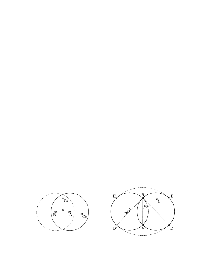
Figure 9: Diagrams for triplet description under 1st and 2nd criterion

We assume that the number of registered showers in an experiment is large enough to adopt it as the average number of showers which would have been registered by the detector in many such runs. The criterion for classifying two showers as a doublet is that the angle between them should be smaller than some given small value $R$. As the expected number of showers within the small angle $R$ around a given direction is $\mu=\rho(\pi R^{2})$ (assuming constant $\rho$ within the circle), the local detection density of doublets can be written as $\rho_{2}=\frac{1}{2}\rho\mu\rme^{-\mu}$ . The factor $\frac{1}{2}$ stands for the fact that both members of a doublet count as one doublet. Of course, the local detection density of singles, where there is no companion within the angle $R$ from the shower considered is $\rho_{1}=\rho\rme^{-\mu}$.
The situation is more complex for the case of a triplet. Two criteria may be distinguished:

1st

- another two showers should be closer than $R$ to the shower considered (in the centre) - criterion applied by AGASA.

2nd

- three showers should be within a circle with diameter $R$.

The 1st criterion is illustrated in the figure B1 (left). In the centre of the right circle there is the shower denoted as A and within the radius R there are another two showers, out of which the shower denoted as B is in a distance $x$ from the first one, in the centre of the left circle. The third shower may be either on the area where the two circles overlap (Ca) or outside it (Cb). In the first case around all three showers a triplet will be found (the same). In the second case the triplet is found only around shower A.
Let S(x) denote the ratio of overlapping area on the figure to the area of the circle. We have the following relations:

$$S(x)=\frac{R^{2}\bigl{[}2\alpha-\sin(2\alpha)\bigr{]}}{\pi R^{2}}$$ (10)

where $\cos(\alpha)=x/(2R)$. The average value of the ratio $S(x)$ equals:

$$\langle S(x)\rangle=2\int_{0}^{R}S(x)\frac{x}{R^{2}}\rmd x=1-\frac{3\sqrt{3}}{4\pi}$$ (11)

Thus, the local detection density of triplets under 1st criterion can be written as :

$$\rho_{3}=\rho\Bigl{[}\frac{1}{3}\langle S(x)\rangle+\Big{(}1-\langle S(x)\rangle\Big{)}\Bigr{]}\frac{\mu^{2}}{2!}\rme^{-\mu}\quad{}$$ (12)

$${}\quad=\frac{1}{3}\rho\Bigg{(}1+\frac{3\sqrt{3}}{2\pi}\Bigg{)}\frac{\mu^{2}}{2!}\rme^{-\mu}$$

The mean numbers of doublets $N_{2}$ and triplets $N_{3}$ detected from all directions are found by integrating their detection densities over the whole solid angle.
We get:

$$N_{2}=\int\rho_{2}(\delta,\alpha)\rmd\Omega=\frac{1}{2}(\pi R^{2})\int(\lambda\eta)^{2}\rme^{-\mu}\rmd\Omega\approx\frac{1}{2}(\pi R^{2})\lambda^{2}\int\eta^{2}\rmd\Omega$$ (13)

$${}N_{3}=\int\rho_{3}(\delta,\alpha)\rmd\Omega=\frac{1}{6}(\pi R^{2})^{2}\Bigg{(}1+\frac{3\sqrt{3}}{2\pi}\Bigg{)}\int(\lambda\eta)^{3}\rme^{-\mu}\rmd\Omega$$

$${}\quad\approx\frac{1}{6}(\pi R^{2})^{2}\lambda^{3}\Bigg{(}1+\frac{3\sqrt{3}}{2\pi}\Bigg{)}\int\eta^{3}\rmd\Omega$$

where we have assumed that $\lambda=const$. Similar consideration as those for detection of triplets under the 1st criterion lead us to the corresponding formulae for quadruplets under the same criterion:

$$\rho_{4}=\rho\Bigl{[}\frac{1}{4}S_{34}+\frac{1}{2}S_{14}+\big{(}1-S_{34}-S_{14}\big{)}\Bigr{]}\frac{\mu^{3}}{3!}\rme^{-\mu}\quad{}$$ (14)

$${}N_{4}=\int\rho_{4}(\delta,\alpha)\rmd\Omega=\frac{1}{6}(\pi R^{2})^{3}\lambda^{4}\cdot 0.66\cdot\int\eta^{4}\rme^{-\mu}\rmd\Omega$$

where $S_{34}$ is the probability that three showers randomly distributed within a circle with a forth shower in the centre will constitute the same quadruplet if any shower out of the three is chosen as the central one. The probability that only one shower out of the three, chosen as the central one, makes the same quadruplet possible is denoted $S_{14}$. It has been found by integration that $S_{34}=0.274$ and $S_{14}=0.270$.
The formulae for detection densities $\rho_{2},\rho_{3},\rho_{4}$ derived above allow for such shower configuration, where the shower B in the figure B1 (left) being a member of a doublet or a triplet is at the same time a member of a triplet or a quadruplet, respectively. After excluding such situations we get for doublets the following formula:

$$\rho^{{}^{\prime}}_{2}=\rho_{2}-\rho\cdot 3\Big{(}1-\langle S(x)\rangle\Big{)}\frac{\mu^{2}}{2!}\rme^{-\mu}\quad{}$$ (15)

Figure B1 (right) illustrates the situation for classifying three showers as a triplet for the 2nd criterion, i.e. three showers have to be within a circle with diameter $R$. The two circles there have diameter $2r=R$. Two showers from directions A and B are at the angular distance AB $<R$. To find the area where the third shower should be we draw the circle of radius $R/2$ through the point A and rotate it around point A until point B is inside the circle, so that points E goes to point E’. Similarly, we rotate the circle around point B until point A is inside the circle (point D goes to D’). To form a triplet the third shower must be located within area E’EDD’.
Let $S_{2}(x)$ be the ratio of the framed area to $\pi R^{2}$ for a given value AB$=x$. It follows that:

$$S_{2}(x)=\big{[}6\alpha+\pi-\sin(2\alpha)\big{]}\frac{1}{4\pi}\quad where\quad\cos(\alpha)=\frac{x}{R}$$ (16)

Taking into account the distribution of distances AB we can calculate the average value of the $S_{2}(x)$:

$$\langle S_{2}(x)\rangle=2\int_{0}^{R}S_{2}(x)\frac{x}{R^{2}}\rmd x=\frac{9}{16}$$ (17)

Further considerations for the local detection density of triplets under the 2nd criterion are only for the case $\mu\ll 1$. So, in a similar way, we get that:

$$\rho_{3}=\rho\frac{1}{3}\langle S_{2}(x)\rangle\frac{\mu^{2}}{2!}=\frac{3}{32}\rho\mu^{2}{}$$

$${}N_{3}=\int\rho_{3}(\delta,\alpha)\rmd\Omega=\frac{1}{6}(\pi R^{2})^{2}\frac{9}{16}\int(\lambda\eta)^{3}\rmd\Omega=\frac{3}{32}(\pi R^{2})^{2}\lambda^{3}\int\eta^{3}\rmd\Omega$$

Numbers of observed doublets, triplets, quadruplets etc undergo Poisson distributions with the corresponding mean (expected) values $N_{2},N_{3},\,(N^{{}^{\prime}}_{2},N^{{}^{\prime}}_{3})$, etc as calculated above. The formulae for the mean numbers of the multiplets have been positively checked in simulations. For the AGASA experiment the following values apply:
$\Theta_{z}=45^{\circ};\varphi=35^{\circ}47^{\prime};R=2.5^{\circ}$
We find that :
$\int\eta\rmd\Omega=\pi(1-\cos^{2}\Theta_{z})=1.57\,sr;\,\int\eta^{2}\rmd\Omega=0.38\,sr;\,\int\eta^{3}\rmd\Omega=0.097\,sr;\,\int\eta^{4}\rmd\Omega=0.0255\,sr$
For the expected value of showers N we use the actual number (registered in the energy range 40 to 80 EeV) - 47 showers and obtained that:
$N_{2}=1.018;\,N_{3}=0.0283;\,N^{{}^{\prime}}_{2}=0.954;\,N^{{}^{\prime}}_{3}=0.0268$ under 1st criterion; $N_{3}=0.0087$ under 2nd criterion; $N_{4}=4.57\times 10^{-4}$ for quadruplets under 1st criterion.
Thus the probability of obtaining two doublets or more and one triplet or more, for the isotropic sky without point sources equals $\bigl{[}1-exp(-N^{{}^{\prime}}_{2})-N^{{}^{\prime}}_{2}\cdot exp(-N^{{}^{\prime}}_{2})\bigr{]}\cdot\bigl{[}1-exp(-N_{3})\bigr{]}=0.247\cdot 0.0279=6.9\times 10^{-3}$. We see that it is mainly the triplet event that makes the isotropy hypothesis very unlikely.

References

References

- [1] Alonso-Herrero, A., Rieke, G.H., Rieke, M.J., Scoville, N.Z., 2000,ApJ, 532, 845
- [2] Al-Dargazelli, S.S., Wolfendale, A.W., Śmiałkowski, A., and Wdowczyk, J., 1996, J. Phys. G 22, 1825
- [3] Berezinsky, V.S. and Grigor’eva 1988, A&A, 199, 1
- [4] Cesarsky, C.J., 1992, Nucl.Phys. B (Proc. Suppl.) bf28, 51
- [5] Cesarsky, C.J., and Ptuskin, V.S., 1993, in Proceedings of the 23rd International Cosmic Ray Conference, 1993, Calgary (University of Calgary, Calgary, Canada), Vol. 2, p. 341.
- [6] Clegg, A.W., Cordes, J.M., Simonetti, J.H., Kulkarni, S.R., 1992, ApJ, 386, 143
- [7] Cox, P., Mezger, P.G., 1989, A&A Rev., 1, 49
- [8] Eade, W.T., Drijard, D., James, F.E., Roos, M., and Sadoulet, B., 1971, Statistical Methods in Experimental Physics (North-Holland Publishing Company: Amsterdam)
- [9] Fisher, N.J., Lewis, T., Embleton, B.J.J., 1993, Statistical Analysis of Spherical Data (Cambridge University Press: Cambridge)
- [10] Greisen, K., 1966, Phys. Rev. Lett., 16, 748
- [11] Han, J.L., Manchester, R.N., and Qiao, G,J, 1999, MNRAS, 306, 371
- [12] Hayashida, N. et al,2000 Preprint astro-phys/0008102
- [13] Heckman, T.M., Armus, L., Weaver, K.A., and Wang,J., 1999, ApJ, 517, 130
- [14] Hibbard, J.E., Yun, M.S. 1999,AJ, 118,
- [15] Kronberg, P.P., 1994, Rep. Prog. Phys. 57, 325
- [16] Lazzati, D. et al, 2001, (astro-ph/0109287), A&A in press
- [17] Medina Tanco, G.A., 2001, ApJ, 549, 711
- [18] Rand, R.J., Lyne, A.G., 1994, MNRAS, 268, 497
- [19] Sanders, D.B., Soifer, B.T., Elias, J.H., Madore, B.F., Matthews, K., Neugebauer, G., and Scoville, N.Z., 1988, ApJ, 325, 74
- [20] Saunders, W. et al2000,MNRAS, 317, 55
- [21] Smith, H.E., Lonsdale, Colin J., Lonsdale, Carol J., 1998, ApJ, 492, 137
- [22] Sofue, Y., Fujimoto, M., 1983, ApJ, 265, 722
- [23] Soifer, B.T. et al1984, ApJLett, 278, 71
- [24] Stanev, T. 1997, ApJ, 479, 290
- [25] Takeda, M. et al1999, ApJ, 522, 225
- [26] Takeda, M. et al2001, in Proceedings of the 27th International Cosmic Ray Conference, 2001, Hamburg, Germany, p345
- [27] Uchihori Y., Nagano M., Takeda M., Teshima M., Lloyd-Evans J., Watson A.A., 2000, Astropart. Phys., 13, 151
- [28] Weiler, K.W., Panagia, N., Montes, M.J., 2001, ApJ, 562, 670
- [29] Wilkinson, P.N., and de Bruyn, A.G., 1990, MNRAS, 242, 529
- [30] Zatsepin, Z.T., and Kuz’min, V.A., 1966, Zh. Eksp. Teor. Fiz. Pis’ma Red., 4, 144