Abundance analysis of targets for the COROT / MONS asteroseimology missions

One of the goals of the ground-based support program for the COROT and MONS/Rømer satellite missions is to select and characterise suitable target stars for the part of the missions dedicated to asteroseismology. While the global atmospheric parameters may be determined with good accuracy from the Strömgren indices, careful abundance analysis must be made for the proposed main targets. This is a time consuming process considering the long list of primary and secondary targets. We have therefore developed new software called vwa for this task. The vwa automatically selects the least blended lines from the atomic line database vald, and consequently adjusts the abundance in order to find the best match between the calculated and observed spectra. The variability of HD 49434 was discovered as part of COROT ground-based support observations. Here we present a detailed abundance analysis of HD 49434 using vwa. For most elements we find abundances somewhat below the Solar values, in particular we find [Fe/H] $=-0.13\pm 0.14$. We also present the results from the study of the variability that is seen in spectroscopic and photometric time series observations. From the characteristics of the variation seen in photometry and in the line profiles we propose that HD 49434 is a variable star of the $\gamma$ Doradus type.

1 Introduction

We first observed HD 49434 (F2V-type) with the ELODIE spectrograph in December 1998 as part of a program with the aim of characterising and selecting potential targets for the asteroseismology space mission COROT (Catala 2001). The strategy is to obtain a number of high resolution, high signal-to-noise spectra of each potential target. For any stars that present line asymmetries or variable line profiles we then carry out more complete monitoring.

Before these observations the star was not considered to be variable, but we discovered systematic low-amplitude variations of the line profiles. Since then we have carried out more extensive spectroscopic and photometric observations.

The purpose of the present paper is to derive the global atmospheric parameters of HD 49434 and to perform an analysis of its photometric and spectroscopic variations.

The French COROT as well as the Danish MONS/Rømer satellite are both asteroseismology missions which will study mostly solar-like stars. Before the launch of these missions (around 2004–5) we need an accurate estimation of the atmospheric parameters and abundances of the proposed target stars. First of all stars with certain parameters may not be suitable for a detailed asteroseismological study, eg. chemically peculiar stars or stars with high rotation rate. Also, in order to carry out the detailed asteroseismological modelling of the stars we need to be able to constrain as many of the global parameters of the stars as possible. Around 10 and 25 primary targets will be chosen for COROT and MONS/Rømer, respectively. It is a very time-consuming process to carry out the abundance analysis of all potential targets manually and we have therefore developed a fast semi-automatic abundance analysis procedure called vwa, which will be described here. The result for HD 49434 is presented, and we will also make comparisons with stars for which abundance analyses have already been carried out manually.

In Section 2 we describe the spectroscopic observations and in Section 3 we describe the vwa software and the result of the abundance analysis. In Section 4 we describe the analysis of the photometric time series, while in Section 5 we analyse the line profile variations in the spectroscopic time series.

2 Spectroscopic observations

HD 49434 is an F2V-type star of magnitude $V=5.74$ (cf. Table 2). We monitored the star spectroscopically from Observatoire de Haute-Provence, using the ELODIE spectrograph, attached to the 1.93 m telescope. The spectrograph is a cross-dispersed spectrograph, providing a complete spectral coverage of the 3 800–6 800 Å region, with a resolving power of about $R=45\,000$ (Baranne et al. 1996).

The first spectroscopic observations of HD 49434 were carried out in December 1998 as part of the search for potential COROT targets. The spectra revealed the presence of variable asymmetries of low amplitude in the line profiles, indicative of non-radial pulsations. Hence, the star was monitored more thoroughly in subsequent observing runs.

On January 26, 2000, HD 49434 was monitored continuously for 90 minutes, with one 5 min spectrum every 7 minutes. The weather and seeing conditions were very good, and the average S/N ratio at 6 000 Å is 250 per velocity bin of 10 $\text{km\,s}^{-1}$.

The star was re-observed on December 10, 2000, almost continuously for 320 minutes, during which as many as 51 five-minute spectra were recorded. The observing conditions of this second monitoring were not as good as the previous one, so that the resulting average S/N ratio at 6 000 Å is only about 170 per pixel per velocity bin of 10 $\text{km\,s}^{-1}$.

The data used for the abundance analysis of HD 49434 are the spectra obtained during the best weather conditions: 12 spectra from January 26, 2000. On the other hand, all of the observed spectra were used for the study of the variability of line profiles. Since the data analysis of the spectra was made by two groups independently, we will describe the data reduction in separate sections, i.e. abundance analysis in Section 3.1 below and the variability of line profiles in Section 5.1.

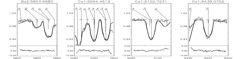
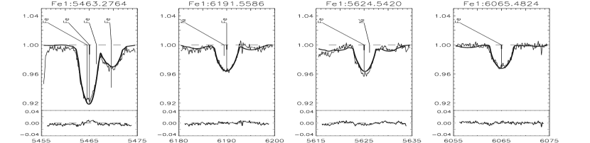
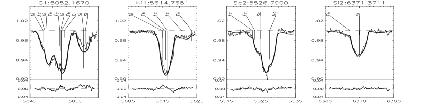
Figure 1: Observed (thin line) and synthetic (thick line) spectrum around twelve lines which were used for the abundance determination. The lower portion of the each plotted line shows the relative difference between the observed and synthetic spectrum. The name of the element and the central wavelength (in Ångstrøm) of each fitted line is given at the top of each plot

3 Abundance analysis

In this section we will describe the abundance analysis of HD 49434. For this purpose we have developed new software for the semi-automatic analysis of spectra. The abbreviation for the software is vwa which explains what the program can determine from the spectrum, i.e. $v\sin i$ of the star, wavelength shift (due to radial velocity), and abundance analysis.

3.1 Data reduction

The bias subtraction, flat fielding, scattered light subtraction, and extraction of the spectral orders were done with iraf. The wavelength calibration was made using a combined Th-Ar comparison spectrum. We made low-order cubic spline fits to make the best continuum estimate. We made sure that the overlap between orders was better than 0.5%. We note that we have not used the region near the hydrogen lines for abundance analysis. The hydrogen lines cover several spectral orders and thus a determination of the continuum level is difficult. One possibility to overcome this problem is to use the average of the continuum level for orders adjacent to the hydrogen lines. This has been done by Lastennet et al. lastennet (2001) and they have estimated the effective temperature from the H$\alpha$ line to be $T_{\rm eff}=7250\pm 250$ K.

The signal to noise of the combined spectrum (12 spectra) at the maximum of a spectral order around 6 000 Å is S/N = 400 per velocity bin of 10 $\text{km\,s}^{-1}$.

3.2 Automatic abundance analysis with vwa

The vwa package can perform three different tasks: Automatic selection of lines for the determination of $v\sin i$, determination of any systematic shift of lines (due to radial velocity), and abundance analysis – the last being the most extensive part of the program.

The first two tasks are not fully implemented in vwa, but $v\sin i$ and $v_{\rm rad}$ can be determined quite easily by comparison of the observed spectrum and several synthetic lines: We convolve the synthetic spectrum with the instrumental profile and different rotation profiles and determine the best fit (we use the program rotate by Piskunov 1992). We find $v\sin i=84\pm 4$ $\text{km\,s}^{-1}$ which is in agreement with Lastennet et al. lastennet (2001) who found $v\sin i=79$ $\text{km\,s}^{-1}$ from the same data set. From the wavelength shifts of non-blended lines we determine the helio-centric radial velocity to be $v_{\rm rad}=-12.3\pm 1.0$ $\text{km\,s}^{-1}$. Gernier et al. (1999) found $v_{\rm rad}=-14.0\pm 0.8$ $\text{km\,s}^{-1}$ from Hipparcos data. We remove the wavelength shift caused by the radial velocity, thus the wavelength scale is the same as the laboratory system.

3.2.1 Input: model atmosphere and atomic data

To use vwa one must calculate an appropriate model for the atmosphere of the star. We have used a modified version of the atlas9 code (Kurucz 1993) as described by Kupka (1996) – see also Smalley & Kupka (1997). In this version of atlas9 the turbulent convection theory in the formulation of Canuto & Mazzitelli (1991, 1992) is implemented.

To calculate the model one needs to know the basic parameters of the star, i.e. $T_{\rm eff},\log g$, and [Fe/H]. These parameters may be estimated from the Strömgren indices of the star by using the program templogg (Rogers 1995) which automatically chooses the most appropriate among several published photometric calibrations. To determine the basic atmospheric parameters of the star templogg then interpolates the de-reddened photometric indices in the atmospheric model grid by Kurucz (1979) with the improvements suggested by Napiwotzki et al. (1993).

For the abundance determination we make use of a complete list of atomic line data for the entire observed spectral range. The line list is extracted from the vald database (Kupka et al. 1999, Ryabchikova et al. 1999) where all lines deeper than 1% of the continuum are included. From the line list (about 13 000 lines for HD 49434) the least blended lines will be selected by vwa.

The selection consists of two steps: 1) Selection based on the analysis of the degree of blending based on the information in the line list from the vald database. 2) These lines are then analysed in the observed spectrum and any “suspicious” lines are rejected. These steps are described in the following two sections.

3.2.2 Selecting lines: atomic line list

For each atomic line extracted from the vald database we examine the line depths of the neighbouring lines. For a given line we examine lines within a certain range specified by the user; for HD 49434 we have used $3.0\times$FWHM of an unblended line ($=3.0\times 2.2$ Å$=6.6$ Å). The line depths of the neighbouring lines are convolved by a Gaussian with a FWHM of $1.5\times$FWHM of an unblended line, i.e. the line depths of lines far away from the central line are suppressed. The selection of lines from the vald line list is based on the degree of blending which is described by three parameters. The user may set his own limits for these parameters, and thus determine which lines are selected. The parameters are: 1) The depth ratio of the central line to the deepest (non-convolved) line. This value must be greater than 1 but can specified by the user (we used 1.35). 2) The number of neighbours with a (convolved) line depth of 25% of the central line must be lower than some limit (we used 5). 3) The sum of the (convolved) line depths must be lower than some number (we used 0.7).

Table 1: Abundances of elements in HD 49434. The weighted mean abundance is given as the logarithm of number of atoms of a given element to the total number of atoms. The weighted standard deviation of the mean is given in parenthesis, $n$ is the number of lines that were used, while the last two columns are the abundances measured for the Sun (Grevesse & Sauval 1998) and the difference between the Sun and HD 49434

Element	Ion	$\log N/N_{\rm tot}$	$n$	$({\log N/N_{\rm tot}})_{\odot}$	$\Delta$
C	i	$-3.46(0.13)$	1	$-3.52$	$+0.06$
Mg	i	$-4.55(0.07)$	3	$-4.46$	$-0.09$
Si	i	$-4.64(0.08)$	2	$-4.49$	$-0.15$
Si	ii	$-4.57(0.06)$	3	$-4.49$	$-0.08$
Ca	i	$-5.51(0.06)$	7	$-5.68$	$+0.17$
Sc	ii	$-8.89(0.11)$	2	$-8.87$	$-0.02$
Ti	ii	$-7.16(0.07)$	2	$-7.02$	$-0.14$
Cr	ii	$-6.45(0.05)$	4	$-6.37$	$-0.08$
Fe	i	$-4.67(0.02)$	16	$-4.54$	$-0.13$
Fe	ii	$-4.43(0.07)$	2	$-4.54$	$+0.11$
Ba	ii	$-9.75(0.09)$	3	$-9.91$	$+0.16$

3.2.3 Rejecting lines: the observed spectrum

When the lines have been selected from the list of atomic lines vwa analyses the observed spectrum in the region around each selected line. The aim is to automatically reject lines that are not suitable for abundance analysis. This is done by fitting a Voigt profile to the observed spectrum. A number of “selection parameters” specified by the user determines if a line will be used: the minimum depth of the fitted profile, the maximum and minimum width of the profile, the maximum value of $\chi^{2}$ for the profile fit, and the maximum flux asymmetry between the left and right part of the observed line.

Optionally the user is presented with a plot of the observed spectrum in a region around each of the selected and rejected lines. The user may then interactively choose if a rejected (accepted) line should be included (rejected) in the abundance analysis. In practice this part of the vwa program creates two lists of the lines that will be rejected / accepted in the final selection of lines to be used for abundance analysis, i.e. these line lists over-rule the automatic selection. The line lists may also be edited manually if, for example, the user already knows which lines he wants to use for the abundance analysis (in accepted line list) – or if the user knows that the atomic parameters of certain lines are known to be uncertain (in rejected line list).

3.2.4 Two methods for abundance determination

The abundance determination is made for each of the selected lines. It can be done by either of two methods: 1) By the measurement of equivalent widths of lines in the observed spectrum which are then given as input to the width9 code by Kurucz atlas9 (1993). 2) By the adjustment of the abundance of the element of the central line of the blend until the computed and observed spectrum around each line match, i.e. they have the same equivalent width. For the computation of the synthetic spectrum we used the program synth (version 2.5) by N. Piskunov (see Valenti & Piskunov 1996).

The first method can only be used for stars where blending is not a problem, i.e. slowly rotating stars ($v\sin i<15$ $\text{km\,s}^{-1}$). The second method is much slower but it is the only option for fast rotators like HD 49434.

3.2.5 Deriving the abundances

For this study we have used the fitting of the abundance in the synthetic spectrum in a region 4 Å on both sides of the central line (the typical FWHM of a single line is about 2.2 Å at 6 000 Å). After all lines have been fitted the user is presented with a plot of the region around each line in which both the synthetic and observed spectrum is shown. Also, all lines with a line depth deeper than 25% of the central line are clearly marked. Several fitted lines are shown in Figure 1. In this “visual inspection” part of vwa the user can click on different sections of the plot which determines if the user thinks the line is fitted correctly, if there seems to be a problem with the continuum level, if the line is severely blended, if the line should simply be ignored, or if the automatic fit has failed. In the last case these lines can be fitted interactively by a separate program (vwa-interact).

The abundance of each element is then calculated using only the lines accepted by the user. Additional constraints on which lines to use may be imposed here, i.e. to use only the least blended lines. For this the “sensitivity” parameter of the line can be used to select the best lines or to give higher weight to certain lines. We define the sensitivity parameter as the change in equivalent width when increasing the abundance, i.e. for a non-blended line this would be the slope of the “curve of growth” near the abundance of the fitted line. The parameter is measured for each line during the automatic determination of the abundance and we find that it depends both on the properties of the line and the degree of blending.

To be specific, the sensitivity, $S_{i}$, for each line $i$, is defined as $S_{i}=\Delta({\rm EQW})/\Delta(\log N/N_{\rm tot})$. Typical values lie in the range 0.3–1.2 mÅ/ dex. For the present data we assume that the measured equivalent widths of all lines are measured with an accuracy of 5%, hence the error estimate of the abundance for a given line lies in the range 0.17–0.04 dex. To get a realistic error estimate for each line one must include systematic errors due to eg. erroneous $\log gf$ values (i.e. oscillator strengths), wrong determination of the continuum level, the possibility of erroneous abundances (or $\log gf$ values) of the lines that blend with the line, and uncertain stellar parameters used for the computation of the atmosphere model.

When calculating the abundance of each element based on several lines we assign weights to each line which depend on the sensitivity of the line. When computing the weights we have added an additional error of 0.07 dex which is the contribution from systematic errors as was discussed above. For the final abundance result of each element we calculate the weighted mean, where the weights are given by $W_{i}^{-1}=(0.05/S_{i})^{2}+(0.07)^{2}$. The standard error on the derived abundance is also calculated using these weights.

3.2.6 Reliability of vwa

We have tested the program on two stars for which careful analyses have already been made: The Sun (Grevesse & Sauval 1998) and FG Vir (A-type star, $v\sin i=21.3\pm 1.0$ $\text{km\,s}^{-1}$; see Mittermayer 2001). For these stars we find good agreement with the previously derived abundances, i.e. within 0.1 dex for all elements.

We note that two future papers which make use of vwa are in preparation, i.e. Rasmussen et al. ngc6134spec (2002) and Bikmaev et al. hd32115 (2002). In the later paper we study two A-type stars and both have low $v\sin i$ (9 and 21 $\text{km\,s}^{-1}$). Thus we may compare the result of vwa with a “classical” abundance determination, i.e. by measuring equivalent widths of non-blended lines. The two methods agree within 0.03 dex for all elements. We conclude that vwa is indeed a reliable tool for fast semi-automatic abundance analysis.

Figure 2: Differential magnitudes of HD 49434 minus comparison star HD 48922 in the Strömgren $b$ band (asterisks). The small points are magnitude differences between the two comparison stars HD 49933 and HD 48922 (shifted to allow comparison). Individual days are marked in every panel as the corresponding HJD

3.3 Abundances for HD 49434

We have estimated the fundamental atmospheric parameters of HD 49434 from the Strömgren photometry given in Table 2. We have used the templogg code (Rogers 1995, see also Kupka & Bruntt 2001) and we find the atmospheric parameters of HD 49434 to be $T_{\rm eff}=7\,300\pm 200$ K, $\log g=4.14\pm 0.20$, and [Fe/H]$=-0.01\pm 0.20$. The quoted errors are approximate and are dominated by the uncertainty from the photometric calibrations.

We determined the microturbulence parameter to be $\xi_{t}=2.1\pm 0.5$ $\text{km\,s}^{-1}$ (cf. discussion in Section 3.3.1). We used macroturbulence $v_{\rm macro}=5.0$ $\text{km\,s}^{-1}$ and $v\sin i=84\pm 4$ $\text{km\,s}^{-1}$. The choice of $v_{\rm macro}$ is not important here, since the width of the lines is dominated by the rotational broadening.

Several lines fitted by vwa are shown in Figure 1. We have also shown the relative difference between the synthetic and observed spectrum. Neighbouring lines with a line depth of at least 25% of the fitted line are also shown. The length of the tick marks show the relative line depth of each neighbouring line compared to the fitted line.

From Figure 1 it can be seen that several lines that were used for the abundance analysis are blended. Due to the high $v\sin i$ of HD 49434 we simply had to use the least blended lines. Our strategy was to determine the Fe abundance accurately from non-blended lines. Consequently, we held the abundance of Fe fixed, and allowed vwa to select lines of other elements that were mildly blended by Fe lines, eg. the Ca lines at 5594.5 and 6102.7 Å. More extreme examples are the C, Ni, and Sc lines at 5052.2, 5614.8, and 5526.8 Å where the lines are heavily blended and the abundance determination is unreliable, i.e. the $S_{i}$ are 0.49, 0.24, and 0.22. If we again assume that the equivalent width is known to 5% the corresponding error is 0.1 dex for the C lines and 0.2 dex for the Ni and Sc lines. In addition, it is difficult to establish the location of the continuum level because the lines are so broad. Realistic error estimates lie in the range 0.2–0.4 dex for these three lines. Note that we did not find enough lines to give a reliable estimate for the abundance Ni and for C we found only one line that was usable.

The result of the abundance analysis is given in Table 1 and for comparison we also give the solar abundances from Grevesse & Sauval sunabund (1998). The abundances and errors are calculated using weights that are estimated from the errors on the individual lines (cf. Section 3.2.5). The error estimates that we give in Table 1 do not include the systematic error due to the uncertainty of the atmospheric model parameters which will be discussed in Section 3.3.1.

Generally we find that the abundances of most elements lie around the Solar value within the error bars. Only for Fe and Ca do we find enough lines (16 and 7) to make a truly reliable estimate of the abundances.

Table 2: Strömgren photometric indices taken from Hauck & Mermilliod (1998) for the four stars used for the HD 49434 observations from Sierra Nevada

Star	$V$	$b-y$	$m_{1}$	$c_{1}$	${\rm H}_{\beta}$
HD 48922	6.77	-0.015	0.142	0.940	-
HD 49933	5.78	0.270	0.127	0.460	2.662
HD 50747	5.45	0.095	0.172	1.131	2.833
HD 49434	5.74	0.178	0.178	0.717	2.755

The Fe abundance is $\log N_{\rm Fe}/N_{\rm tot}=-4.67\pm 0.02$ from 16 Fe i lines (we quote the internal weighted error; the internal RMS scatter is 0.18 dex). If we assume that the photospheric hydrogen and helium abundance is the same in HD 49434 and the Sun this abundance corresponds to [Fe/H] $=-0.13\pm 0.14$ (including systematic errors). This agrees roughly with the result from the Strömgren $m_{1}$ index which yields [Fe/H] $=-0.01\pm 0.20$.

An interesting result is the ratio [Ca/Fe] $=+0.30\pm 0.21$ which is a quite high value for a star with Solar-like abundances.

We note that we have adjusted the $\log gf$ for the Ca ii line at 5857.451 Å line by comparing with the solar spectrum, i.e. from $\log gf=0.257$ to $0.550$. The $\log gf$ values for the Si lines are determined solely from theoretical calculations. Therefore we have computed the synthetic spectrum for the Si-lines we have used – using the solar abundance – and comparing this with the observed solar spectrum. We find that the $\log gf$ values seem to be right for the lines we have used.

Lastennet et al. lastennet (2001) have determined fundamental atmospheric parameters of HD 49434 by comparison of the observed and synthetic photometric colours. The star is among the nine potential COROT targets stars they have studied. From the combination $(B-V)$, $(U-B)$, $(b-y)$ they find $\log g=4.0\pm 0.4$, $T_{\rm eff}=7\,240\pm 100$ K and [Fe/H]$=-0.1\pm 0.2$ (from Table 2 and Figure 7 and 8 in Lastennet et al. 2001). Thus, the metallicity they find is in agreement with our result from spectroscopy and all the fundamental parameters are in agreement with the estimates based on Strömgren photometry.

We finally note that HD 49434 is included in the $\Delta a$ photometry catalogue of bright B and A stars by Vogt et al. (1998) but they find no evidence for the star being chemically peculiar.

3.3.1 Accuracy of the derived abundances

The errors quoted in Table 1 for the abundances are the weighted internal errors (cf. Section 3.3.1). Here we will discuss the error contribution from the uncertainty of the atmospheric model parameters. The atmospheric model we used for the final abundance result have the parameters $T_{\rm eff}=7\,300$ K and $\log g=4.1$. To investigate the effect of the choice of atmospheric model we calculated Fe abundances for models with $T_{\rm eff}=7\,100,7\,300,7\,500$ K and $\log g=4.1$ and one model with $T_{\rm eff}=7\,300$ and $\log g=4.3$. We find that the effect of increasing $\log g$ by $0.2$ dex decrease the Fe abundance by about $0.04\pm 0.05$ dex (sd. of mean) which is not significant. On the other hand, if we increase the temperature of the atmospheric model by $200$ K we find an increase of Fe by $0.10\pm 0.05$ dex, i.e. a significant effect.

Another input parameter for the calculation of the synthetic spectrum is the microturbulence. The value used in the calculation of the Kurucz atmosphere model does not affect the derived abundances significantly, but when calculating the synthetic spectrum the effect is indeed significant. When changing the microturbulence the change in equivalent width depends on the strength of the line. By using this fact, one can adjust the microturbulence until the abundance of individual lines do not correlate with equivalent width. We could not do this very accurately due to the high rotational velocity of HD 49434. Thus, we estimate the microturbulence to be $\xi_{\rm t}=2.1\pm 0.5$ $\text{km\,s}^{-1}$.

We find that when increasing $\xi_{\rm t}$ by 0.5 $\text{km\,s}^{-1}$ the abundance of Fe decreases by $0.10\pm 0.04$ dex, i.e. a significant contribution to the uncertainty of the abundance.

We conclude that the contribution to the error of abundances due to uncertain model atmosphere parameters, i.e. $T_{\rm eff}$ and microturbulence, is of the order 0.14 dex. For a realistic estimate of the abundance of elements in HD 49434 this contribution must be added to the internal errors (sd. of mean) given in Table 1. For example for the metallicity of HD 49434 we get [Fe/H] $=-0.13\pm 0.14$, i.e. the uncertainty of the model parameters is the main error source.

Figure 3: Power spectra corresponding to the variable star HD 49434 minus the comparison star HD 48922, in the upper panel, and that corresponding to the comparison stars HD 49933 minus HD 48922 in the bottom panel. The scales are milli-magnitudes and cycles/day

4 Strömgren photometry time series

We have observed HD 49434 with a Strömgren photometer on the 0.9m telescope at Sierra Nevada near Granada, Spain. We used a $45"$ diaphragm to observe HD 49434 and the comparison stars HD 48922=C1, HD 49933=C2, and HD 50747=C3. The star HD 49933 is a V = 5.78 double system with a faint companion of magnitude V = 11. This last star was included within the diaphragm because of its proximity but had no influence on the final differential photometry. The Strömgren parameters for the observed stars are given in Table 2.

Figure 4: Location of HD 49434 (star symbol) in the HR diagram together with the known $\delta$ Scuti (circles, Rodríguez & Breger 2001) and bona fide $\gamma$ Dor (triangles, Handler & Kaye 2001) pulsators. The edges of the $\gamma$ Dor region around $(b-y)_{0}=0.2$ are from Handler (1999). The absolute magnitude of HD 49434 is $M_{V}=2.73\pm 0.07$ and is derived from its Hipparcos parallax (ESA 1997)

Continuous photometric time series of comparison stars HD 48922, HD 49933 and HD 49434 were made in order to remove the sky transparency fluctuations to be able to see the variations of the target star. Magnitude differences between HD 49933 and HD 48922 are constant within 3.7 mmag (rms) and clear intrinsic variations can be seen for HD 49434. The light curve is shown in Figure 2.

The time series consist of data from nine nights spread unevenly over one month starting on July 2001. Unfortunately the weather conditions were not good during our first night of observation and HD 49434 was observed again a week later. Observations were possible only three weeks later where the star was included in a program where other targets were also measured. Thus the dedicated observing time was limited to only a few measurements but the data could be used to confirm the long-term variations that were seen in the first days.

In total the time series consists of 295 data points in the four Strömgren bands ($uvby$). In Figure 2 we show the time series of HD 49434 - HD 48922 (target - comparison star 1) and HD 49933 - HD 48922 (comparison star 2 - comparison star 1). The magnitude differences are plotted for the Strömgren $b$ band.

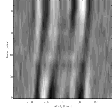
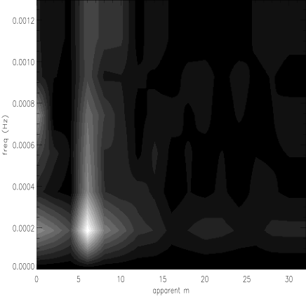
Figure 5: The residual of the mean profile for the January 2000 series. Left: in velocity – time space; the maximum amplitude is of the order of $3\times 10^{-3}$; Right: Spectral power density of the same data, in apparent order – frequency space, after the 2D Fourier transform

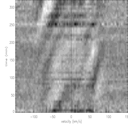
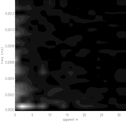
Figure 6: The same as Figure 5 but for the December 2000 series; the maximum amplitude of the residuals is of the order of $4\times 10^{-3}$

From Figure 2 it is clear that the intrinsic photometric variations are associated with HD 49434. At first sight the star does not seem to have periodic variations. A power spectrum was calculated in order to search for possible frequency components which is shown in Figure 3. It can be seen that with the present data, no clear discrete frequency components are present. Instead the low frequency region has a significant contribution for HD 49434 which is not seen for the comparison stars.

This behaviour is typical among the recently discovered $\gamma$ Dor stars (Zerbi et al. 1999) which are g-mode pulsators. We believe that HD 49434 is a variable star of this type: the star is classified as a main sequence F2-type star from Strömgren photometry and its position in the Hertzsprung-Russell diagram in Figure 4 confirm our hypothesis. Because we have not detected any clear periodicity it is not possible to test the phase differences among the different photometric colours which is a clear signature of the non-radial pulsating nature of the $\gamma$ Dor stars – see Garrido garrido2000 (2000) for details.

5 Spectroscopic monitoring of HD 49434

In the following we will discuss the analysis of the time series of spectra of HD 49434 to look for any systematic variation of line profiles.

5.1 Data reduction

All data were reduced on-site, using the automatic INTER-TACOS procedure (Baranne et al. 1996), resulting in wavelength-calibrated, flat-field corrected spectra. Each spectrum is segmented into 67 segments corresponding to the 67 orders of the spectrograph present on the detector. We then performed a large scale normalisation of the overall spectrum, so that the resulting spectra are normalised to unity all across the covered wavelength domain, even though some local problems still remain with this normalisation on the edges of the orders.

The ELODIE spectrograph provides a wide enough spectral coverage to give access to a large number of photospheric lines. In order to take advantage of this, and to fully exploit the information contained in these numerous photospheric lines, we used the Least-Square Deconvolution (LSD) technique (Donati et al. 1997) to analyse the variations of a “mean” photospheric line. In this method, a line pattern function is constructed, containing all the lines supposedly present in the spectrum as Dirac functions, with heights set to the central line depths as calculated by Kurucz’s (1979) “SYNTHE” program. The observed spectrum is then deconvolved with this line pattern function, yielding a “mean” photospheric line profile. With this technique, line blends are automatically taken into account when all the lines present in the spectrum are considered. Note that the depth of the resulting “mean” line has no physical meaning, but that time variations of this depth, as well as line profiles can be accurately analysed with this technique. We used a Kurucz model for $T_{\rm{eff}}=7\,000$ K and log $g=4$, sufficiently close to the values derived in this paper, for constructing the line pattern function.

A total of 1700 lines were finally used in this analysis. In the following of this work, we shall call “mean” photospheric line, the line constructed with the LSD technique, while the adjective “average” will be reserved for time averages of line profiles.

All mean profiles in each series were normalised to the same equivalent width. This procedure eliminates the effects of the large scale variations of the mean line profile, due for instance to normalisation problems that may vary from spectrum to spectrum. The time average of the mean profiles was then constructed for each series, and subtracted from the mean line profiles of the series.

We then performed a two-dimensional Fourier transform analysis, following the method described in Kennelly et al. (1996). This method is well suited for the analysis of the spectroscopic signature of non-radial pulsations. Each line profile was interpolated on a grid representing stellar longitudes, transforming velocities across the line profile into longitudes on the stellar equator using the relation $v-v_{r}\;=\;v\sin i\;\sin\phi$, where $v$ is the velocity in the profile, $v_{r}$ is the radial velocity of the star, measured to be $v_{\rm rad}=-12.3\pm 1.0$ $\text{km\,s}^{-1}$, $\phi$ is the corresponding stellar longitude, and $v\sin i$ is the projected rotation velocity of the star, estimated to be $84\pm 4$ $\text{km\,s}^{-1}$.

For the time series from January 2000, the spectra were recorded at constant time intervals during the whole monitoring, while a few short gaps exist in the December 2000 series. For this latter series, prior to the 2D Fourier transform, we had to build up a grid of constant time intervals, filling the gaps during which no spectrum was obtained with null data.

After these steps, the data were submitted to a 2D Fourier transform, resulting in a representation of the data in the (frequency – apparent $m$) space. The apparent $m$ is related to the structure of the modes present at the stellar surface, without being identical to the usual azimuthal order $m$, since the apparent $m$ depends for instance on the inclination angle $i$ of the rotation axis of the star with respect to the line of sight. The apparent $m$ is nevertheless indicative of the surface structure of the modes detected.

5.2 Detected variability of spectral lines

Figure 5 (and Figure 6) presents the results of this analysis for the series from January 2000 (and December 2000). At both epochs we detect the presence of line profile perturbations, crossing the profile from blue to red. Such perturbations are most probably the signature of non-radial pulsation modes at the stellar surface. The Figures 5 and 6 suggest the presence of one or several high-degree modes. These modes are particularly obvious in the January 2000 series, owing to the high signal-to-noise ratio of the spectra, while they are less conspicuous, although present without doubt, in the lower quality December 2000 data. The amplitudes of the residuals are of the order of 2–3$\times 10^{-3}$ at both epochs. They can be easily detected thanks to the very high signal-to-noise ratio (S/N) of the LSD mean line profiles combining hundreds of spectral lines, which reach S/N=3 000 in the December 2000 series and S/N=6 000 in the January 2000 series.

These modes seem to be long-period modes. This is particularly clear in Figure 6 (right), where the frequency of the detected modes are at the resolution limit of our dataset, i.e. 0.1 mHz, indicating a period longer than 160 minutes, that is to say longer than half the time span of the monitoring. These results therefore confirm those of the photometric observations, and suggest that HD 49434 is probably a variable of the $\gamma$ Doradus type.

The modes we detect in the January 2000 series are high-degree modes, with an apparent order of 6. In the December 2000 series, our lower quality data still indicates non-radial modes, but with more power on the apparent order 2, some signal still appearing at apparent order 8.

6 Conclusions and future prospects

We have presented the detailed abundance analysis of HD 49434. The analysis could not be made by simple equivalent width measurements since most lines are blended, because the star has high projected rotational velocity. We have described the vwa software which selects the least blended lines and derive abundances semi-automatically.

We find that the metallicity of HD 49434 is somewhat below the Solar value, i.e. [Fe/H]$=-0.13\pm 0.14$. The quoted error includes the estimated error due to the uncertainty of the atmosphere parameters, especially $T_{\rm eff}$ and microturbulence.

The metallicity we find agrees with the results from Strömgren photometry and the work by Lastennet et al. lastennet (2001) who have compared observed and synthetic photometric colours. When taking into account the uncertainty of the basic atmosphere parameters the accuracy of vwa is only slightly more accurate than the photometric methods. The advantage of analysing the spectra with vwa is that we obtain estimates for several elements.

We have already used vwa for the analysis of several other stars which will be published soon (Bikmaev et al. 2002, Rasmussen et al. 2002). In the paper by Bikmaev et al. we have analysed two A-type stars, which have low $v\sin i$. Thus we have made a detailed comparison of the result obtained with vwa and with the “classical” method based on equivalent width measurements of non-blended lines – the agreement is excellent for nearly all lines (abundances $<0.03$ dex).

With the confirmation that vwa can be used for reliable semi-automatic abundance analysis we will proceed to use the software for analysis of the proposed main targets for the asteroseismology satellite missions COROT and MONS/Rømer: the spectra have already been obtained.

For our future use of vwa we expect that for stars with low $v\sin i$ ($<$ 40–50 $\text{km\,s}^{-1}$) it will be possible to constrain the atmospheric parameters (eg. microturbulence and $T_{\rm eff}$) by adjusting these so the abundances found from lines of the same element do not correlate with the line parameters (eg. equivalent width and excitation potential). For stars with higher $v\sin i$ ($>100$ $\text{km\,s}^{-1}$) the selection of atomic lines for abundance analysis becomes exceedingly difficult. For such stars the metallicity and the basic parameters must be determined mainly from photometric colours, but it is still important to obtain spectra to be able to put constraints on $T_{\rm eff}$ (from the hydrogen lines) and $v\sin i$. For example, stars with too high $v\sin i$ may not be suitable for seismology since this will make the analysis much more complex.

In the present paper we have also presented the photometric light curve of HD 49434 based on observations during part of nine nights over a period of one month. We find that the star is indeed variable with excess power around 1-5 cycles per day, but no periodic signal could be found from the limited data set. We have also analysed the spectroscopic line profiles which show evidence for long-period variability at low amplitude. This behaviour is characteristic for the $\gamma$ Dor variables, and we propose that HD 49434 is indeed a variable of this type. A longer time series is needed to be able to detect any periodic pulsation signal.

The star has been chosen as a main target for COROT which means that the star will be observed for around 150 days. We will then be able to probe the interior of this star in detail by using seismic techniques. To do this one needs to constrain the fundamental parameters of the star which indeed has been aim of the work presented here.