UU Aqr from high to low state

In this paper we present Physical Parameter Eclipse Mapping (PPEM) of UBVRI eclipse light curves of UU Aqr from high to low states. We used a simple, pure hydrogen LTE model to derive the temperature and surface density distribution in the accretion disc. The reconstructed effective temperatures in the disc range between 9 000 K and 15 000 K in the inner part of the disc and below 7 000 K in the outer parts. In the higher states it shows a more or less prominent bright spot with $T_{\mbox{\scriptsize eff}}$ between about 7 000 K and 8 000 K.
The inner part of the disc ($R<0.3R_{\scriptscriptstyle L1}$) is optically thick at all times, while the outer parts of the disc up to the disc edge ($0.51\pm 0.04R_{\scriptscriptstyle L1}$ in the high state and $0.40\pm 0.03R_{\scriptscriptstyle L1}$ in the low state) deviate from a simple black body spectrum indicating that either the outer disc is optically thin or it shows a temperature inversion in the vertical direction.
While during high state the disc is variable, it appears rather stable in low state. The variation during high state affects the size of the optically thick part of the disc, the white dwarf or boundary layer temperature and the uneclipsed component (originating in a disc chromosphere and/or cool disc wind), while the actual size of the disc remains constant. The difference between high and low state is expressed as a change in disc size that also affects the size of the optically thick part of the disc and the presence of the bright spot.
Using the PPEM method we retrieve a distance for UU Aqr of 207$\pm$10 pc, compatible with previous estimates.

1 Introduction

Cataclysmic variables (CVs) are close interacting binaries in which the white dwarf, the primary component, accretes matter from a red dwarf companion (for extensive reviews on CVs see Warner 1995 or Hellier 2001). Depending on the strength of the magnetic field of the white dwarf and the mass accretion rate from the secondary the system geometry and physics of accretion varies. We deal in this paper with a white dwarf primary that has a negligible magnetic field. In this case the matter drawn from the secondary is accreted through an accretion disc. A relatively high accretion rate as in the nova-like UU Aqr leads presumably to a steady state disc that does not show outbursts like low accretion rate dwarf novae.

UU Aqr is a relatively bright CV with a magnitude of 13.5 and an orbital period of $3^{h}56^{m}$ that was first reckognized as an eclipsing CV by Volkov, Shugarov & Seregina (1986). This makes it a relatively easy target to observe and indeed it has been observed in the IR (Dhillon et al. 2000, Huber & Howell 1999), in the UV (White et al. 1995) as well in the optical wavelength range. Optical photometry was reported by Honeycutt, Robertson & Turner (1998) and Baptista, Steiner & Cieslinski (1994, hereafter BSC) while optical spectroscopic data were analysed by Baptista et al. (2000), Kaitchuck et al. (1998), Hoard et al. (1998), Diaz & Steiner (1991), and Haefner (1989). It has not been detected in the ROSAT PSPC All Sky Survey (Verbunt et al. 1997) like two thirds of the nova-like systems in Verbunt et al.’s list. These observations have led to relatively well-defines system parameters, like the inclination angle $i=78^{\circ}$, mass ratio $q=0.30$ and white dwarf mass ${\cal M}_{wd}=0.67{\cal M}_{\odot}$.

Since it shows single peaked emission line profiles, Baptista, Steiner & Horne (1996, hereafter BSH) first proposed that UU Aqr is a member of the SW Sex type CVs. Other features of these objects are phase-dependent absorption components, hardly eclipsed emission lines, and large phase shifts between photometric and spectroscopic ephemerides. Doppler maps are bright in the lower left quadrant and the eclipses are V shaped, indicating a flat temperature profile (e.g. Warner 1995). Furthermore, these systems do not usually show the rotational disturbance of an eclipsed accretion disc.

UU Aqr shows all these features (for a summary see Baptista et al. 2000). Haefner (1989) already found the emission line profiles to be variable and states that it “indicates several sources of emission within the system: symmetrical profiles as well as strong asymmetries or even double peaks are present”. The variability could be caused by a variable disc wind which sometimes is substantially reduced allowing the double peaked emission from the disc to be seen. Kaichuck et al. (1998) and Baptista et al. (2000) suggest that the emission lines originate in a chromosphere and a disc wind and/or that the disc has a disc anchored magnetic propeller in which the gas is ejected in all directions. Hoard et al. (1998) propose a detailed model for the emission and absorption sites in the disc.

BSH discovered that UU Aqr changes between high and low states on a timescale of a couple of years and that the main difference is the presence of a bright spot in the high state and lack of it in the low state. In addition, Honeycutt et al. (1998) observed so-called “stunted” outbursts which have the duration of a dwarf nova outburst, but only small amplitudes of less than a magnitude (compared to 2-3 mag in dwarf novae outbursts).

The aim of this paper is to investigate quantitatively the difference between high and low states and the variation within those states. We analysed BSH’s eclipse light curves individually and combined them in six sub-states to minimize the influence of flickering and flaring.

A second objective was to determine the distance to UU Aqr using the PPEM method and compare it to previous estimates. BSC determined a distance of 270$\pm$ 50 pc by fitting the white dwarf flux. In BSH they used a method similar to cluster main sequence fitting and arrived at a distance of 200$\pm$30 pc.

2 The data and system parameters

The data set was previously presented by BSC and BSH. The 37 eclipses of UU Aqr observations were taken with the 0.6m and the 1.6m telescopes of the Laboratorio Nacional da Astrofisica (LNA/CNPq) in Brasil. Further details about the data aquisition and reduction can be found in BSC.

Apart from analysing only the high and low state data, we also analysed the individual light curves with the PPEM method. The aim was to retrieve more detail using the PPEM algorithm, since this method allows us to obtain the distributions of temperature and surface density over the disc using the information of the five colours simultaneously.

3 The PPEM analysis

The Physical Parameter Eclipse Mapping method was presented by Vrielmann, Horne & Hessman (1999, hereafter VHH). An overview of applications of this method to various systems is given in Vrielmann (2001). Vrielmann, Stiening & Offutt (2002a) and Vrielmann, Hessman & Horne (2002b) show applications to V2051 Oph and HT Cas, respectively. We will give here only a very short description of the method, the interested reader is referred to the above articles for more details.

The idea is based on the Eclipse Mapping developed by Horne (1985) which uses the eclipse profile in order to reconstruct the light distribution in the eclipsed source, i.e. the white dwarf and the accretion disc. Hereby, a Maximum-Entropy-Method (MEM) helps to choose the distribution (or map) with the least structure still compatible with the observed data.

PPEM goes a step further in that it uses multi-band light curves in order to reconstruct distributions of physical parameters, e.g. the temperature and surface density of the eclipsed object. This means a spectral model for the emissivity of these objects has to be adopted.

In this study, we use white dwarf spectra and a simple, pure hydrogen spectrum for the accretion disc as described in the next Section. Future studies (see Vrielmann, Still & Horne 2002c) will include more sophisticated disc model, like those computed by Hubeny (1991).

3.1 The spectral model used for PPEM

For the reconstruction of the physical parameters we used a uniform, pure hydrogen LTE slab including only free-free and bound-free emission (as described in more detail in VHH):

$$I_{\nu}(T,\Sigma)=B_{\nu}(T)\cdot\left[1-e^{-\frac{\tau_{\nu}}{\cos i}}\right]$$ (1)

where $B_{\nu}(T)$ is the blackbody spectrum, $i$ the inclination angle and $\tau_{\nu}$ the optical depth, calculated as:

$$\tau_{\nu}=\kappa_{\nu}\Sigma$$ (2)

where $\kappa_{\nu}(\rho,T)$ is the mass absorption coefficient for hydrogen, including atomic and H^- bound-free and free-free contributions. The mass-density $\rho$ is calculated from $\Sigma$ and $T$ using the vertical half-thickness ($c_{s}$: sound speed, $V_{\mbox{\tiny Kepler}}$: keplerian velocity):

$$H(R,T)=\frac{c_{s}(T)R}{V_{\mbox{\tiny Kepler}}}$$ (3)

For $\frac{\tau}{\cos i}\gg 1$, Eqn. 1 transforms into the optically thick case $I_{\nu}\approx B_{\nu}(T)$. For the optically thin case $\frac{\tau}{\cos i}\ll 1$, Eqn. 1 reduces to $I_{\nu}(T)\approx\frac{\tau}{\cos i}\cdot B_{\nu}(T)$.

We choose the parameters temperature $T$ and surface density $\Sigma$ to be reconstructed. From the reconstructed maps in $T$ and $\Sigma$ we can e.g. calculate the effective temperatures, the optical depth, or the Balmer Jump strength, i.e. the ratio $I_{\nu}(T,\Sigma)/B_{\nu}(T)$ (see Section 4.1).

Although this model is simple, it is very useful, because it allows us to diffentiate between optically thick and optically thin parts, or more generally, disc regions with emissivity resembling or deviating from the black body spectrum. Furthermore, for typical temperatures and surface densities in real discs, LTE and the pure hydrogen assumption are good approximations. On the other hand, the opacity in the cooler regions of real disc will be typically much higher, leading to overestimated temperatures for disc regions cooler than about 6300 K. For a more detailed discussion on the applicability of the model see Vrielmann et al. (2002b).

Thus, deviations from BB emission (Balmer jump in emission or absorption) are attributed to optical depth effects. If such deviations are instead due to temperature gradients in the disc atmosphere, our simple model will produce systematic errors. In realistic discs, it is possible that the inner part of the disc shows a stellar-type decreasing temperature with disc height while the outer regions show a chromospheric-type temperature inversion. If this is the case our simple model will fail.

3.2 PPEM distance estimates

Figure 1: The entropy of the reconstructions (a measure of smoothness) as a function of the assumed distance. For each trial distance the data were fitted with $\chi^{2}/N=2$ (high state, squares) and 1.25 (low state, circles). The dashed lines are parabolic fits to the data, they peak at 206 pc and 208 pc, respectively.

Using the PPEM method we determined a new distance estimate for UU Aqr. The distance-entropy relation for the fits to the high and low state data is plotted in Fig. 1 and shows clear peaks at 206 pc and 208 pc. Due to lack of any true constraint to weigh the two values we take the simple average of the distance (207 pc). In Vrielmann et al. (2002b) we show a test case using an artifical non-axisymmetric disc and derive a distance 2.5 % larger than the assumed true distance. We have not included reddening in these calculation, however, as BSH point out, the reddening is nearly negligible and would change the distance by at most 5 pc. We estimate therefore the total error of the distance to 10 pc with the assumption that our spectral model describes the true emissivity reasonable well. For the following calculations we used the trial distance (and BSH’s distance) of 200 pc which should give basically identical results.

Our distance estimate is in very good agreement with BSH’s value of $200\pm 30$ pc using a method similar to cluster main sequence fitting for the accretion disc, however, it is only marginally compatible with their distance derived from a fit to the white dwarf flux by BSC. As BSC remark, they may have over-estimated the radius of the white dwarf and included (part of) the boundary layer in its estimate.

This again shows that the PPEM method is in principle a very good method to estimate distances of real objects. However, as described in Vrielmann et al. (2002b) in the case that the disc has patches that lead to a covering factor less than unity the PPEM distance would be overestimated. The fact that our estimate agrees with BSH’s and is smaller (rather than larger) than the white dwarf estimate by BSC leads to the conclusion that the disc is probably not patchy.

3.3 The light curves

Figure 2: The six binned light curves in UBVRI with the fits, the residuals and the uneclipsed components.

While BHS have binned the light curves by year of observation and then separated into high and low states, we rearranged the light curves according to decreasing out-of-eclipse flux in V. Since this did not yield a clear separation into two different states, i.e. the high and low state, instead, we recognized six categories and binned them accordingly into 6 sub-states (see Tab 1).

Table 1: Eclipse numbers (see BSC) sorted into six bins (sub states) according to the out-of-eclipse flux in V. Column 3 gives an estimate of the average flux in mJy (errors are 0.3 mJy) and column 4 the corresponding magnitude.

Bin	Eclipse No.	$<F>$	$<m>$
1	8592, 9025, 8512	13.9	13.55
2	8574, 8458, 8591, 8586, 8531	13.2	13.6
	10823
3	8525, 8585, 8042, 8524, 8140	12.6	13.65
4	8030, 8530, 8518, 10822, 10828	11.8	13.7
	8024, 8744, 15200, 9031, 10829
5	6739, 15212, 6745, 6744	10.8	13.8
6	15213, 15207	10.2	13.9

However, checking which light curves contributed to which sub-state, we can rediscover the high and low states recognized by BHS: the high state consisting of the sub-states 1 to 4 and the low state of sub-states 5 and 6. The eclipses in sub-state 5 and 6 were taken in different years or seasons, i.e. in 1988 and 1992, than the eclipses in the other sub states (taken in 1989 and 1990, with the exception of eclipse #15200). A comparison with Honeycutt et al.’s (1998) data shows that in July 1992 UU Aqr was in a low state (however, not in the lowest possible) with a V magnitude of about 13.8, while at other times it varies around a V magnitude of 13.5. Some ten days later (perhaps 30, definitely 50) UU Aqr experienced a so-called “stunted” outburst. Unfortunately, there is no more overlap between the two data sets. Apparently, the systems either rests in a low state or varies within the brighter 4 sub-states.

We cannot exclude that the odd eclipse (e.g. #8512 (sub-state 2?), #8531 (sub-state 3?), #10823 (sub-state 3?)) might be missclassified (to a sub-state too high), because the light curves usually only cover the immediate eclipse and not enough signal before and after the ingress and egress, respectively, to decide whether the flux just preceding or following the eclipse was contaminated by a flicker or a broad hump.

During the high state the system often changes in flux. The average time scales for dropping from one sub-state to another is about five orbital cycles or more. However, on two occasions the system dropped from sub-state 1 to 4 within 6 cycles. The rise from one sub-state to another, even jumping an intermediate sub-state, however, can occur much quicker, sometimes within one cycle.

In the case of the eclipses #8530 and #8531, during which the system jumped two (or at least one) sub-states upwards, an inspection of the original light curves clearly shows an increase in the redder passbands (i.e. in BVRI). Furthermore, the eclipse #8531 is much shallower (also especially in the redder filters) and shows indications of a bright spot. We must therefore conclude that the system indeed changed significantly within this particular orbit, possibly due to an increase in the uneclipsed component (disc wind).

The binned light curves in UBVRI are shown in Fig. 2, together with the fits, the residuals and the uneclipsed component. All light curves show a shallower egress than ingress, indicative of a bright spot, however, the asymmetry is strongest in the light curves of the higher sub-states.

The amount of flickering and noise in the binned light curves is inversely proportional to the number of individual light curves in the respective bin number.

4 Results

4.1 The reconstructed accretion disc

We reconstructed two-dimensional temperature $T$ and surface density $\Sigma$ distributions of the accretion disc. As explained in VHH, the parameters can only be reconstructed with a certain accuracy, depending on the value of each parameter (i.e. the location in the parameter space). Usually, the temperature can be reconstructed with a better accuracy than the surface density. (We strongly recommend the reader to study the article VHH). As explained in Vrielmann et al. (2002a) and (2002b) the effective temperature, which also depends on the total emission (the quantity that is fitted), is usually relatively acurately reproduced. Furthermore, this parameter is also usually dealt with in theoretical studies.

Another useful tool to investigate the accretion disc physics is the parameter $I_{T,\Sigma}/I_{BB}$, where $I_{T,\Sigma}$ is the intensity derived from the $T,\Sigma$ maps and $I_{BB}$ the black body temperature derived from the $T$ map alone. This parameter measures the deviations of the observed spectrum from a blackbody spectrum of same temperature and, differently from $T$ and $\Sigma$, is a model-independent quantity. It may also be understood as a measurement of the Balmer Jump strength. According to the adopted spectral model, where this value reaches unity the disc is optically thick and in regions where the emissivity deviates from the black body it assumes values $0<I_{T,\Sigma}/I_{BB}<1$. In extremely dim regions (which can de facto mean outside the true disc radius) this ratio can also reach nearly unity, because of the small values for $I_{T,\Sigma}$ and $I_{BB}$ involved.

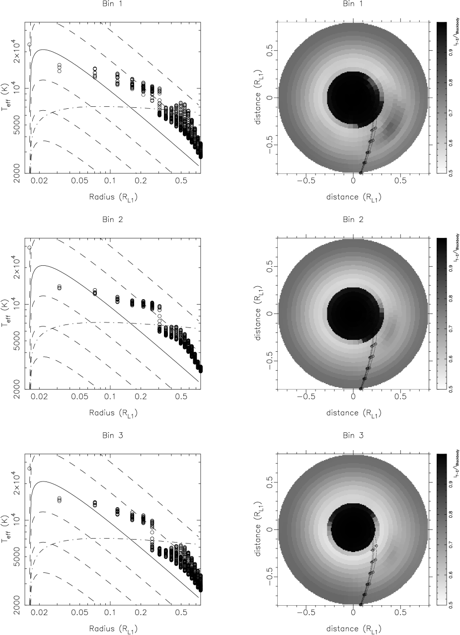
Figure 3: Left: The effective temperature distribution derived from the reconstucted temperature and surface density distributions for the first three bins. The dashed lines give theoretical steady state effective temperature distributions for mass accretion rates $\log\dot{\cal M}=13$ to 18, the one for $\dot{\cal M}=10^{16}$gs^-1is drawn solid for reference. The dashed-dotted line indicates the critical effective temperature $T_{{\mbox{\scriptsize eff}},{\rm A}}$ according to Ludwig, Meyer-Hofmeister & Ritter’s (1994) critical mass accretion rate $\dot{\cal M}_{\rm A}$. Right: The Balmer Jump strength ($I_{T,\Sigma}/I_{BB}$) distribution derived from the reconstucted temperature and surface density distributions for the first three bins. A ratio of unity (black areas) means the emitting material is optically thick.

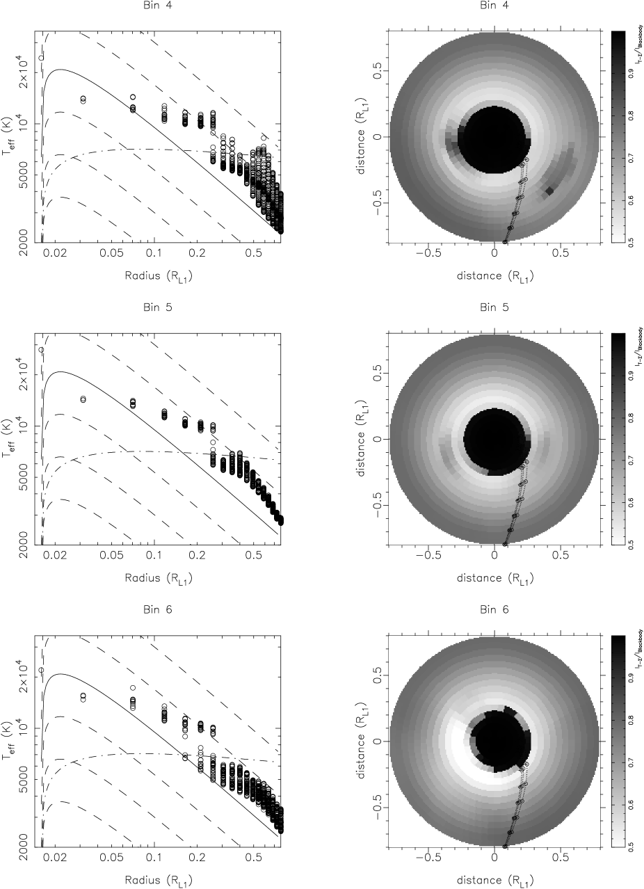
Figure 4: As Fig. 3 but for the last three bins.

Fig. 3 and 4 show the effective temperature and Balmer Jump strength ($I_{T,\Sigma}/I_{BB}$) distribution derived from the reconstructed temperature and surface density distributions. The pattern for $I_{T,\Sigma}/I_{BB}$ and the effective temperature (not shown) are similar, indicating that hot regions are emitting optically thick and cooler regions deviate from a black body source of same temperature. Most prominent is the clear transition between the optically thick inner part of the disc with a radius of between 0.3$R_{\scriptscriptstyle L1}$ and 0.25$R_{\scriptscriptstyle L1}$ in the highest and lowest sub-states, respectively, and the outer, optically thin regions (see also Section 4.2.3).

We remark that the observed deviations from blackbody emission in the outer disc regions, interpreted in the framework of our simple spectral model as the signature of optically thin emission, can have a different interpretation, namely, that the outer parts of the disc show a vertical structure with a temperature inversion possibly caused by irradiation from the hot, inner disc regions.

The maps show that the bright spot, expected to appear where the accretion stream hits the disc, is strongest in the hottest states and curiously in the intermediate state (bin 4). The bin 4 light curve in Fig. 2 shows a dip during egress at phase 0.08 and a kink at phase $-0.04$ that must be responsible for the spot in the reconstructed map. It is unlikely that this spot is due to an unfortunate contamination of flickering, because 10 light curves contributed to this bin and any such arbitrary effect should have been averaged out.

The radial distribution of the effective temperature $T_{\mbox{\scriptsize eff}}(R)$ follows the steady state distribution only in the outer parts of the disc. In the inner, optically thick, part of the disc $T_{\mbox{\scriptsize eff}}(R)$ flattens out, irrespective of the sub-state. This flattening in the innermost part with radii $R<0.1R_{\scriptscriptstyle L1}$ can only partly be attributed to the MEM smearing (see VHH). BSH also found a flattening in their maps of UU Aqr and Rutten, van Paradijs & Tinbergen (1992) in SW Sex and V1315 Aql. It appears to be a feature of SW Sex stars. However, another interpretation is that the Balmer Jump in the inner part could be in absorption. Since our simple model cannot handle this, the effective temperatures in the inner disc and subsequently also the mass accretion rates might be underestimated.

The mass accretion rate in the outer regions of the disc varies between $5\times 10^{16}$gs^-1 in the highest sub-state (1 and 2) via $3.5\times 10^{16}$gs^-1 in the intermediate sub-states (3 to 5) and $2.5\times 10^{16}$gs^-1 in the lowest (6). However, in the bright spot it can reach values of up to $3\times 10^{17}$gs^-1. Since the effective temperature distribution is rather flat in the inner disc, it drops to about $4\times 10^{15}$gs^-1 in the innermost part of the disc in all sub-states.

Fig. 3 and 4 also show the critical effective temperature $T_{{\mbox{\scriptsize eff}},{\rm A}}(R)$ derived from the critical mass accretion rate $\dot{\cal M}_{\rm A}(R)$ as given by Ludwig et al. (1994). In nova-likes the effective disc temperatures should lie above this critical value as to prevent any dwarf nova-type outbursts. The plots show that the inner optically thick part of the disc is at all times well above this critical limit. However, the outer parts fall partly below, especially in regions away from the bright spot. This might be the reason for the mini-outbursts observed by Honeycutt et al. (1998).

The size of the optically thick region (see also Section 4.2.3), the presence of the bright spot and the mass accretion rate suggest that in sub-states 1 and 4 the disc is most active. It is possible that the activity starts at the bright spot and only slowly works itself through to the inner parts of the disc (#8518 to #8524 and #8030 to #8042) or that the disc emission drops suddenly (#8512 to #8518 and #9025 to #9031) without immediately affecting the presence of the bright spot.

We performed PPEM on all individual light curves for comparison and statistical uses. Images of the intensity ratio maps and radial effective temperature profiles can be viewed at http://pinguin.ast.uct.ac.za/$\sim$sonja/uuaqrmaps.html. A postscript file of the maps can also be downloaded.

In the following Sections we focus on the white dwarf temperature, the uneclipsed component and the disc radius as reconstructed for various sub-states.

4.2 Various aspects of the reconstructions

4.2.1 The white dwarf

Table 2: The white dwarf temperature in the various sub-states of the accretion disc $T_{wd,sub}$ and the average of the reconstructed white dwarf temperatures derived for the individual light curves $<T_{wd}>$. The error for $T_{wd,sub}$ must be estimated to about 1000 K, the standart deviation for $<T_{wd}>$ is given in the last column. The second column lists the no. of eclipses contributing to each bin.

Bin	No. of eclipses	$T_{wd,sub}$	$<T_{wd}>$	$\sigma(<T_{wd}>)$
1	3	23000	24200	1300
2	6	29200	24200	3500
3	5	26600	27533	2900
4	10	24300	23900	5700
5	4	28100	30300	8800
6	2	22000	30600	1900

The white dwarf temperature $T_{wd}$ as reconstructed for the light curves in the various sub-states is given in Tab. 2. We also list an average of the white dwarf temperatures reconstructed after applying the PPEM method to the individual light curves. In principle these temperatures should be roughly identical, however, flickering and noise in the individual light curves affect the resulting individual $T_{wd}$’s. This is most likely the case for the two light curves in bin 6. Furthermore, we could not always fit the light curves to the same $\chi^{2}$ without introducing severe artifacts. This might also influence the exact value of the reconstructed $T_{wd}$’s, as probably happened in bin 2. We therefore rely more on the values of $T_{wd}$ for the various substates rather than the individual $T_{wd}$’s. The error of the $T_{wd,sub}$ is about 1000 K. This is determined by the change in $\chi^{2}$ due to an artificial change of the white dwarf temperature in the otherwise original reconstructed maps.

The $T_{wd}$’s derived for the four highest sub-states show a minimum for the lowest and highest ones. If one would assume the four sub-states to represent a time sequence, this could be understood as a reaction of the white dwarf temperature due to delayed accretion onto the white dwarf: In the hottest state the white dwarf temperature is practically identical to the low state temperature (sub-state 6). The accretion disc, however, experiences enhanced accretion into the bright spot, as evident from the prominent bright spot and reacts rather quickly. The white dwarf can only slowly react to this change in the accretion disc. Only in the second sub-state can the enhanced accretion onto the white dwarf be seen, the white dwarf temperature is at its maximum. For the next two bins the white dwarf cools down, however, the enhanced accretion during bin 4 leads to another white dwarf temperature maximum in bin 5. Bin 6 represent low states in which the disc and the white dwarf are at their lowest activity.

As beautiful as this scenario looks, there are, however, a few problems. First of all, the timescale for a change in the temperature of the white dwarf is too short. The white dwarf cannot cool down by a few 1000 K within a few orbits (less than a day) as would be required for both jumps from sub-state 1 to 4 for eclipses #8512 to #8518 and for #9025 to #9031 within 6 orbits.

Secondly, checking the light curves, the system does not always seem to cycle through all sub-states (e.g. cycling from 4 to 3 and back: #8518 $\rightarrow$ #8524 $\rightarrow$ #8525 $\rightarrow$ #8530), or seems to spend some time in one intermediate sub-state before it suddenly jumps into a higher one (e.g. it rests in substate 2 during eclipses #8586 and #8591 before it jumps within one orbit to sub-state 1 (#8592)).

Since the sequences are unfortunately not taken continuously or with a constant time intervall it is difficult to determine how exactly the system behaved. Explicitly, we cannot always determine whether the system was on its way into a high state or low state. In this regard, it would be of great interest to gather light curves for several consecutive nights.

It seems more likely that the actual location for the variable source is the boundary layer around the white dwarf, since it is unlikely that the white dwarf can cool so quickly. The fastest cooling rate quoted by Sion (1999) is about 400-500 K per day (for RX And) instead of a few thousand Kelvin per orbit (4$h$) as would be necessary for UU Aqr. Although PPEM has a better constraint to determine the spatial distribution of physical parameters, we am still left with some ambiguity. The maximum entropy also prefers a solution with one bright image pixel (e.g. the white dwarf) to more structure distributed over a range of pixels, e.g. the inner part of the disc. Furthermore, the white dwarf pixel value is not smeared out with the surrounding disc pixels (VHH) which which will enhance this effect. The idea of a variable boundary layer also supports the consequences we find for the uneclipsed component as described in the following section.

The white dwarf temperatures are in general compatible with Sion’s (1999) results who finds an average white dwarf $T_{\mbox{\scriptsize eff}}$ of 24,100 K for non-magnetic systems.

4.2.2 The uneclipsed component

Table 3: Uneclipsed component in the filters UBVRI for the reconstruction of the 6 binned light curves. The last two rows give the expected flux of a dwarf of the indicated type at the distance of 205 pc.

Bin/Flux(mJy)	U	B	V	R	I
1	1.44	2.21	0.79	0.83	1.01
2	1.69	2.69	1.04	0.87	1.15
3	2.56	3.39	1.91	1.84	2.34
4	1.56	2.19	0.66	0.73	0.78
5	1.36	1.80	0.26	0.24	0.11
6	2.21	2.45	1.04	1.04	1.43
M4V	–	–	0.06	0.21	0.81
M6V	–	–	0.002	0.01	0.09

Figure 5: The uneclipsed component in the various sub-states as indicated in the graphs (thin lines). The points with error bars (full circles: sub-states 1,3,5; full triangles: sub-states 2,4,6, respectively) give the average of the uneclipsed spectra from the individual reconstructions and are largely compatible with the sub-state uneclipsed spectra. Furthermore, the error bars give an indication of the reliability of the sub-state spectra. For comparison the flux of M4V (thick solid line) and M6V (thick dashed line) dwarf stars are drawn at the bottom of each graph.

The uneclipsed component for the various filters and bins is given in Tab. 3 and Fig. 5. The uneclipsed flux consists of the flux from the secondary and other sources in the system that are never eclipsed, like a disc wind or a chromosphere as suggested by Baptista et al. (2000).

The secondary has a mass of $0.20\pm 0.07{\cal M}_{\odot}$ (BSC) which fits to a M(4$\pm$1)V dwarf star according to Kirkpatrick & McCarthy (1994). Table 3 gives the flux of an M4V dwarf star at a distance of 205 pc. If the secondary is a M4V dwarf, then the reconstructed I-band flux in sub-state 5 is too small. However, the test in Appendix A shows that the uneclipsed flux in all filters might be underestimated. Furthermore, the CVs analysed by Beuermann et al. (1998) with an orbital period similar to that of UU Aqr have a spectral type of M$4\pm 1$.

Another constraint for the spectral type of the secondary comes from the K light curve (Huber 2001, private communication). The out-of-eclipse light curve ($m_{K}\sim 12$ mag) shows orbital variation that can be attributed to the ellipsoidal change in surface area of the secondary and an eclipse of the secondary by the outer edges of the disc. The full amplitude is 0.14 mag or 13% of the minimum flux. An M4V dwarf has a K magnitude of 7.80 (Kirkpatrick & McCarthy 1994) and would therefore contribute 13% to the minimum K flux. If the secondary has a spectral type of M4V this means that it were fully eclipsed in order to cause the observed orbital variation. This cannot be the case. Only if it is brighter than a typical M4V dwarf can the ellipsoidal shape cause such strong orbital variation. The secondary should therefore have an earlier spectral type than M4V.

Our estimated limit for the secondary of 13% of the K flux is compatible with Dhillon et al.’s (2000) upper limit of 55% derived from the lack of absorption features in the IR spectra.

The remaining part of the uneclipsed component must arise in other parts of the system. As we show in Appendix A the excess in the uneclipsed B flux is an artifact due to the spectral model we used with PPEM. The cause is most likely that the size and optical depth of the bright spot is influenced by maximum entropy smearing. Disregarding the strong B-band flux the uneclipsed spectrum could be compatible with optically thin emission or more likely of an extended source with varying temperature and density. This could be from a disc chromosphere or a disc wind or a combination of both as suggested by Baptista et al. (2000).

A look at the changes of the uneclipsed contribution through the various sub-states show that the uneclipsed component seems to react even slower than the white dwarf temperature or boundary layer (if the substates do represent a time sequence). Only in sub-state 3 there is a significant increase in the uneclipsed component.

With the assumption that although the absolut flux units are errorneous, the shape of the uneclipsed spectrum in the UVRI passbands are represented correctly (see Appendix A), we can make a cautious statement about the variation of the uneclipsed spectrum with substate. The difference in flux in the various high sub-states appears to be constant with respect to wavelength except for a slight increase in the I-band. This is also true for the two low states and means that the varying part of the uneclipsed component either consists of a nearly wavelength independent plus a cool source or a moderately hot plus a cool source. The cool source could be the outer regions of a disc wind driven vertically out of the disc, as suggested already by BSC and calculated by Pereyra & Kallman (2000). Any fluctuations in the disc wind will be most noticeable in the outer, cooler regions of the disc wind.

IR spectra taken by Dhillon et al. (2000) show that the emission lines profiles of B$\gamma$ (Brackett series of H I), B$\delta$ and He I $\lambda 2.0587\mu$m are single-peaked. This is understandable if the emission lines originating in the cool disc wind dominate over the line emission from the disc. This disc wind is possibly triggered by the changes in the mass accretion rate.

4.2.3 The disc radius

Figure 6: The radius of the optically thick part of the disc (squares with error bars) and the radius of the bright spot (asterixes with error bars). Th bright spot radii must be increased by about 0.07$Rl$, judging from tests with artificial data. $1\leavevmode\nobreak\ R_{\scriptscriptstyle L1}=5.2\times 10^{10}$ cm.

Table 4: Radii of features in the accretion disc: $R_{cen}$ is the central optically thick region (errors are 0.02$R_{\scriptscriptstyle L1}$), $R_{spot}$ the radius of the bright spot (tests show these values must be increased by about 0.07$R_{\scriptscriptstyle L1}$) and $R_{I}$ an estimate of the disc radius using the intensity distribution in the I-band filter (errors are 0.05$R_{\scriptscriptstyle L1}$). The latter is an upper limit for the disc size.

Bin	$R_{cen}$	$R_{spot}$	$\sigma(R_{spot})$	$R_{I}$
1	0.28	0.50	0.09	0.71
2	0.28	0.46	0.06	0.61
3	0.26	0.51	0.03	0.66
4	0.26	0.57	0.11	0.71
5	0.23	0.4	0.03	0.57
6	0.22	–	–	0.63

From the maps in Fig. 3 and 4 we measure the radius of the optically thick part of the disc and the bright spot, where applicable, i.e. for all but the last bin. The values are listed in Table 4.

A test with artificial data shows (Appendix A) that the spot location is reconstructed at a slightly larger azimuth (judging from the brightness maximum in the spot) and a slightly smaller radius, by about 0.07$R_{\scriptscriptstyle L1}$ (this value decreases with decreasing $\chi^{2}$ and increasing signal-to-noise factor). The true spot locations will thus be at a slightly larger radius than given in Table 4.

The spot radius increases from sub-state 1 to 4. However, since the error bars are rather large, a constant spot radius of about $R_{spot}(high)=0.51R_{\scriptscriptstyle L1}\pm 0.04R_{\scriptscriptstyle L1}(=(2.6\pm 0.2)\times 10^{10}$ cm) is also compatible with the data. Only in the sub-state 5 does the spot radius decrease slightly to $R_{spot}(low)=0.40R_{\scriptscriptstyle L1}(=2.1\times 10^{10}$ cm).

The spot radius should be a good measure of the disc radius. However, due to the lack of any traces of the bright spot in the lowest sub-state we unfortunately cannot determine a comparable measure for the disc size. Analysing the intensity maps we can only estimate an upper limit of the disc radius, as given in Table 4.

Fig. 6 also gives the radius of the transition zone between the inner optically thick accretion disc and the optically thin outer parts (or the radius at which the temperature inversion in the outer disc becomes dominant). It decreases from $0.28R_{\scriptscriptstyle L1}$ in the highest sub-states to $0.22R_{\scriptscriptstyle L1}$ in the lowest. Baptista et al. (2000) find a transition zone at between $0.2R_{\scriptscriptstyle L1}$ and $0.3R_{\scriptscriptstyle L1}$ in which the emission lines show P Cygni profiles for which either the absorption (H$\delta$, He I $\lambda$5876) or emission (H$\gamma$, H$\beta$, H$\alpha$) component is stronger. Their result is therefore compatible with ours.

4.3 Discussion

4.3.1 The accretion disc

Our disc radii ($R_{spot}(high)=0.51R_{\scriptscriptstyle L1}(+0.11R_{\scriptscriptstyle L1}-0.04R_{\scriptscriptstyle L1})$ and $R_{spot}(low)=0.40R_{\scriptscriptstyle L1}(+0.1R_{\scriptscriptstyle L1}-0.03R_{\scriptscriptstyle L1})$) are somewhat smaller, but compatible with previously derived values. Harrop-Allin & Warner (1996) find disc radii of UU Aqr of $0.61<R_{d}/R_{\scriptscriptstyle L1}<0.88$ in the high state and $0.48<R_{d}/R_{\scriptscriptstyle L1}<0.72$ in the low state while BSC find $\sim 0.72R_{\scriptscriptstyle L1}$ and $\sim 0.38R_{\scriptscriptstyle L1}$, respectively. The eclipse map in BSH’s Fig. 9b, however, shows the spot in the high state at $0.56\pm 0.12R_{\scriptscriptstyle L1}$, compatible with our estimate. Harrop-Allin & Warner as well as BSC determined the disc size by the bright spot contact phases and appear to give slightly too large results, while Eclipse Mapping seems to derive too small ones. However, the radii derived from eclipse mapping techniques can be improved with better signal-to-noise ratio data and better fits (using more appropriate spectral models) as tests show. Furthermore, Eclipse mapping methods use the information of the whole eclipse profile and are therefore minimally interfered by flickering. On the other hand, accretion stream overflow could in principle cause the bright spot to appear closer to the white dwarf than the actual disc edge. For example, Horne’s (1999) model for SW Sex stars includes mass overflow.

Since the disc radius does not seem to change with the variations during high state, the inner optically thick disc must be directly responsible for the changes in the out-of-eclipse flux. The variation in the size of the optically thick part of the disc is presumably directly correlated to a redistribution of the mass.

UU Aqr’s disc is so close to the critical mass accretion rate that it is not surprising that the system appears so variable as already pointed out by BSH. It is not only switching between low to high states, but also varying in the high state. Furthermore, it shows stunted outbursts during low state as observed by Honeycutt et al. (1998). Our analysis suggests that these stunted outbursts might be caused in the outer disc in which the temperatures fall below the critical value. If this is correct they are due to a disc instability like normal outbursts in dwarf novae, however, shorter and with lower amplitude, because the temperatures in the outer disc easily reach the critical values and the temperatures in the inner disc are already above the critical limit. The cause of the variation between high and low state, however, is more likely a varying mass accretion rate as suggested by BSH. It would be very valuable to know if the normal outbursts as indicated by Volkov et al.’s (1986) observations start during high or low state and how frequently they occur.

4.3.2 The disc wind

Baptista et al. (2000) give a detailed discussion on the presence of a disc wind and chromosphere in UU Aqr (we do not want to repeat their argumentation). Our observational results are compatible with this most likely scenario. Our results also favour a geometrically extended (maybe spherical or equatorial) source that could be an outflowing gas and/or chromosphere covering areas of different temperatures rather than a collimated jet.

In Doppler tomographs a disc wind with a velocity of $v_{w}$ would appear as a ring with a diameter of the projected velocity ($v_{w}\cos i$). (In high resolution Doppler maps one could possibly detect a small hole in this ring at $(v_{x}=v_{w}\cos i,v_{y}=0)$ due to the exclusion of the eclipse phases.) Since the inclination angle $i$ is large, this ring would be small and occupy the central regions of the Doppler maps. The Doppler maps of Kaitchuck et al. (1998) show emission from the central regions apart from the accretion disc and bright spot contributions. While a clear ring-like structure cannot be seen, the half-orbit maps support such emission feature. Improved signal-to-noise spectra are highly desireable in order to decide about this type of feature in the Doppler maps.

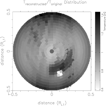
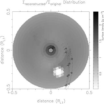
Figure 7: Ratio of reconstructed to original parameter maps for the test case. The bright area indicates the location where the original spot was placed, the dark, slightly overlapping region where spot was reconstructed.

Appendix A Tests with artificial discs

Table 5: Flux of the original and reconstructed uneclipsed component in the filters UBVRI for the test case (in mJy).

	U	B	V	R
original	0.09	0.069	0.69	0.16
reconstructed	0.04	0.03	0.00	0.07

Figure 8: Uneclipsed component for the original (circles) and reconstructed (crosses) accretion disc in the test case.

In order to explain the excess in the B-band flux we performed a test of the PPEM method with artificial data. We constructed an axisymmetric disc with a gaussian bright spot at a radius of $0.3R_{\scriptscriptstyle L1}$, a sigma of 0.02$R_{\scriptscriptstyle L1}$ and an azimuth of 20^∘, calculated the light curve in UBVR with 112 data points between $-0.1$ and 0.1. To this light curve we added a signal-to-noise of 50 and a constant factor of 0.01 mJy to the error bars in order to keep a minimum error for small fluxes, e.g. during eclipse. The uneclipsed component was set artificially to an optically thin spectrum.

This light curve was the input for the PPEM programme and could be fitted to a $\chi^{2}$ of 1.1. Fig. 7 shows the ratios of the reconstructed map to the originals, highlighting the locations of the spot. The reconstructed spot is located roughly at the right position, but at a slightly smaller radius of $0.23R_{\scriptscriptstyle L1}$ and slightly larger azimuth of 30^∘ than the original one. Furthermore, the spot is smeared out due to the maximum entropy (MEM) constraint. Such a spreading of the spot could also be realistic, so in reconstructions of real data one cannot give a precise size for the azimuthal extension of the spot.

The uneclipsed component was reconstructed as shown in Table 5 and Fig. 8. Most striking is the fact that the reconstructed flux is lower than the original one. This is due to the MEM smearing leading to larger maps and/or smoother gradients in the outer parts of the disc. This leads to more flux in the outer, uneclipsed regions of the disc.

Except for the B-band flux, the general shape of the uneclipsed spectrum is recovered relatively well. The reason for the excess in the reconstructed B-band flux in due to the smearing of the spot, leading to larger parts of the disc being (nearly) optically thick. Our model spectrum therefore underestimates the B-band flux in the disc, leading to an increase in the uneclipsed component in order to fit the out-of-eclipse flux.