The Star Formation History and the spatial distribution of stellar populations in the Ursa Minor Dwarf Spheroidal Galaxy

Abstract

As a part of a project devoted to the study of the Ursa Minor dSph, the star formation history of the galaxy is presented in this paper. The analysis uses wide field photometry, encompassing about $1^{\circ}\times 1^{\circ}$ (the total covered area being $0.75$ deg²), which samples the galaxy out to its tidal radius. Derivation of the SFH has been performed using the synthetic partial model technique.

The resulting SFH shows that Ursa Minor hosts a predominantly old stellar population, with virtually all the stars formed earlier than 10 Gyr ago and 90% of them formed earlier than 13 Gyr ago. Nevertheless, Ursa Minor color-magnitude diagram shows several stars above the main, old turn-off forming a blue-plume (BP). If these stars were genuine, main-sequence stars, Ursa Minor would have maintained a low star formation rate extending up to $\sim 2$ Gyr ago. However, several indications (relative amount and spatial distribution of BP stars and difficulty to retain processed gas) play against this possibility. In such context, the most reliable hypothesis is that BP stars are blue-stragglers originating in the old population, Ursa Minor hence remaining the only Milky Way dSph satellite to host a pure old stellar population. A marginally significant age gradient is detected, in the sense that stars in outer regions are slightly younger, in average.

The distance of Ursa Minor, has been calculated using the magnitude of the horizontal-branch and a calibration based on Hipparcos data of main sequence sub-dwarfs. We estimated a distance $d=76\pm 4$ Kpc, which is slightly larger than previous estimates. From the RGB color, we estimate a metallicity $[Fe/H]=-1.9\pm 0.2$, in agreement with a previous spectroscopic determination. No metallicity gradients have been detected across the galaxy.

1 Introduction

Dwarf spheroidal (dSph) galaxies are objects of high cosmological significance. In generic hierarchical clustering scenarios for galaxy formation, such as cold dark matter dominated cosmologies (White & Rees 1978; Blumenthal et al. 1984; Dekel & Silk 1986), dwarf galaxies should have formed prior to the epoch of giant galaxy formation and would be the building blocks of larger galaxies. The dSphs observed today would be surviving objects that have not merged within larger galaxies. Therefore, unveiling their underlying structure could provide important clues about process of dwarf galaxy formation that are now observed at high red-shifts. Local Group galaxies offer the only opportunity of studying their evolution in great detail through the observation of their resolved stellar populations, which are fossil records of the star formation history (SFH).

DSph companions of the Milky Way were historically considered as old systems inhabited by globular cluster-like, population II stars (Baade 1963). However, later works revealed traces of intermediate-age stars, such as carbon stars (Aaronson & Mould 1980; Mould et al. 1982; Frogel et al. 1982; Azzopardi, Lequeux & Westerlund 1986) and bright AGB stars (Elston & Silva 1992; Freedman 1992; Lee, Freedman & Madore 1993; Davidge 1994; but see also Martínez-Delgado & Aparicio 1997). More recent studies, based on the analysis of color-magnitude diagrams (CMDs) using synthetic CMDs, have shown that dSph are objects with complex and varied SFHs (Mighell 1997; Martínez-Delgado, Gallart, & Aparicio 1999; Gallart et al. 1999a; Hernández, Gilmore & Valls-Gabaud 2000; Aparicio, Carrera & Martínez-Delgado 2001) and the idea that no two dSphs could be identified to have similar SFHs has become popular.

As part of a bigger project devoted to the study of the Ursa Minor dSph galaxy (see Martínez-Delgado et al. 2001, 2002), we present in this paper the results on the SFH of this galaxy. Our data sample the galaxy out to $40^{\prime}$ from its center, which is of the order of its tidal radius (see Irwin & Hatzidimitriou 1995; Kleyna et al. 1998; Martínez-Delgado et al. 2001). Ursa Minor is the second closest dwarf spheroidal galaxy satellite of the Milky Way ($d=69$ Kpc) and was discovered in the Palomar survey by Wilson (1955). Previous works show an old system similar, in age and abundance, to the ancient metal-poor Galactic globular cluster M92 (Olszewski & Aaronson 1985; Mighell & Burke 1999) and owning a well populated, predominantly blue horizontal-branch (HB) (see e.g. Cudworth, Olszewski & Schommer 1986; Kleyna et al. 1998). Martínez-Delgado & Aparicio (1998) pointed out the possibility that a marginal intermediate-age stellar population could exist in the galaxy, associated to the blue-plume present in its CMD. Olszewski & Aaronson (1985) and Mighell & Burke (1999) derived distance moduli of $(m-M)_{0}=19.0\pm 0.1$ and $19.18\pm 0.12$ respectively, from a sliding fit to the M92 ridge line. As for the metallicity, it has been recently estimated by Shetrone, Côté, & Sargent (2001), from spectroscopic measurements of giant stars, to be $[Fe/H]=-1.9\pm 0.11$.

Martínez-Delgado et al. (2001) have shown evidences that Ursa Minor is in a process of tidal disruption. This motivates the spatially extended study of the SFH that we present here. Before us, Hernández et al. (2000) (see also Valls-Gabaud, Hernández, & Gilmore 2000) have obtained the SFH for the very central part of Ursa Minor using deep, but small field ($\sim 2\farcm 5\times 2\farcm 5$) HST data. They find a stellar population mainly composed of stars older than 10 Gyr.

The paper is organized as follows. In §2, the observations and photometric reduction are presented. In §3, the CMD of Ursa Minor is discussed, followed by the estimation of the distance and metallicity. The rest of the paper is mainly devoted to the derivation of the SFH and the discussion of possible evolution scenarios for Ursa Minor, to which §4, 5 and 6 are devoted. Finally, the main results of the paper are summarized in §7.

2 Observations and data reduction

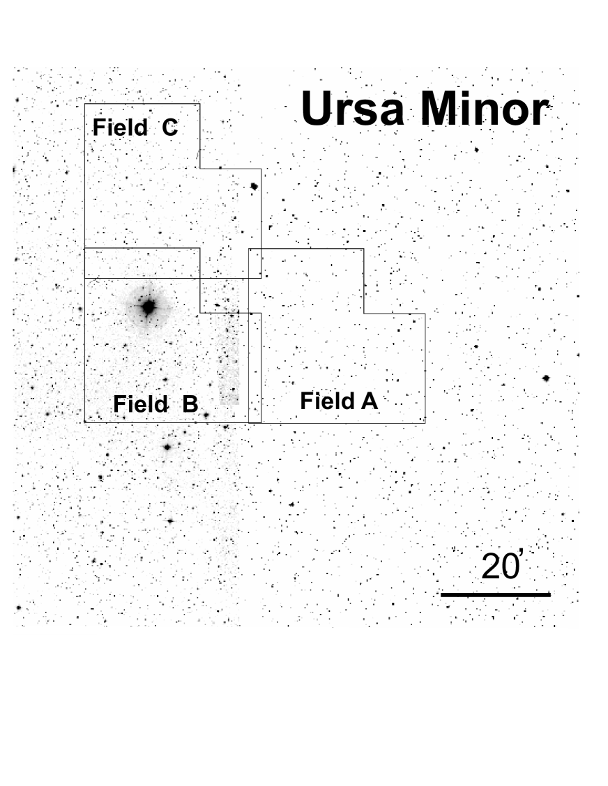
Figure 1: Digitized Sky Survey image of the Ursa Minor region. The observed fields are over-plotted. The galaxy is centered about the center of Field A. North is up, East is left.

The observations of Ursa Minor were carried out in $B$, $V$, $R$ and $I$ Johnson-Cousins filters with the 2.5 m Isaac Newton Telescope (INT) at Roque de los Muchachos Observatory in La Palma and, with the 0.8 m, IAC-80 telescope at Teide Observatory in Tenerife. In the INT we used the WFC installed at the prime focus, that holds four $2048\times 4096$ pixels EEV chips. The scale is $0.33^{\prime\prime}$/pix, which provides a total field of about $35^{\prime}\times 35^{\prime}$. Three fields were observed in $B$ and $R$ filters encompassing a region of about $1^{\circ}\times 1^{\circ}$, with a total covered area of about $0.75$ deg². Table 1 provides a summary of the observations. Figure 1 shows the observed fields. The field containing the center of the galaxy (field A) was also observed in $V$ and $I$. These data will be used to estimate the distance and metallicity (see §3). Observations with the IAC-80 telescope were done to obtain the standard transformations for these bands. A Thomson $1024\times 1024$ chip was used with a scale of 0.43^′′/pix, covering a total area of nearly $7.5^{\prime}\times 7.5^{\prime}$.

The images were processed in the usual way. Bias and flat-field corrections were done with IRAF. DAOPHOT and ALLSTAR (Stetson 1994) were used to obtain the photometry of the resolved stars. Transformation into the standard photometric system requires several observations of standard star fields in such a way that standards are measured in all four chips of the WFC. In practice, we observed three fields from Landolt (1992) in the four chips and used them to calculate relative photometric transformations from each chip to the central one (chip 4). Then, a larger number of standard star fields were measured in chip 4 during the observing run to calculate both nightly atmospheric extinctions and the general transformation into the standard Johnson–Cousins system. In total, 170 measurements of 38 standards were made during the observing run of May 1998. Summarizing, the transformations from each chip to chip 4 are:

$$(b_{4}-b_{1})=0.329+0.02(B-R);~{}~{}~{}~{}\sigma=0.005,$$ (1)

$$(r_{4}-r_{1})=0.837-0.307(B-R);~{}~{}~{}~{}\sigma=0.010,$$ (2)

$$(b_{4}-b_{2})=0.443-0.006(B-R);~{}~{}~{}~{}\sigma=0.007,$$ (3)

$$(r_{4}-r_{2})=0.833-0.268(B-R);~{}~{}~{}~{}\sigma=0.008,$$ (4)

$$(b_{4}-b_{3})=0.367+0.021(B-R);~{}~{}~{}~{}\sigma=0.008,$$ (5)

$$(r_{4}-r_{3})=0.739-0.233(B-R);~{}~{}~{}~{}\sigma=0.008,$$ (6)

where sub-indices refer to chips, lower-case letters stand for instrumental magnitudes, and capital letters for Johnson-Cousins magnitudes. The $\sigma$ values correspond to the fit dispersion at the barycenter of point distribution; hence they put lower limits to the zero-point errors.

Transformations from chip 4 instrumental magnitudes measured at the top of the atmosphere into Johnson-Cousins magnitudes are given by:

$$(B-b_{4})=24.553-0.061(B-R);~{}~{}~{}~{}\sigma=0.009,$$ (7)

$$(R-r_{4})=24.393+0.257(B-R);~{}~{}~{}~{}\sigma=0.010,$$ (8)

where, as before, lower-case letters refer to extinction-free, instrumental magnitudes and capital letters to Johnson–Cousins magnitudes.

The central field (field A in Fig. 1) of Ursa Minor was also observed with the INT in $V$ and $I$ in June 1999. This run was not photometric, for which the IAC-80 telescope was used in May 2001 to obtain the photometrical calibration. Fifteen standards from Landolt (1992) and several secondary standards defined in the central region of Ursa Minor (covered by chip 4 in the INT observations) were observed to this aim with the IAC-80. The resulting transformation equations for the IAC-80 were:

$$(V-v_{\rm IAC80})=21.110+0.055(V-I);~{}~{}~{}~{}\sigma=0.009$$ (9)

$$(I-i_{\rm IAC80})=21.064+0.076(V-I);~{}~{}~{}~{}\sigma=0.006$$ (10)

while the final transformation for the INT observations (chip 4) resulted:

$$(V-v_{\rm 4})=24.13+0.04(V-I);~{}~{}~{}~{}\sigma=0.02,$$ (11)

$$(I-i_{\rm 4})=24.21+0.02(V-I);~{}~{}~{}~{}\sigma=0.02,$$ (12)

As formerly, lower-case letters refer to instrumental magnitudes and capital letters to Johnson–Cousins magnitudes.

Finally, dispersions of the extinctions for each night are about $\sigma=0.01$ for each filter. Aperture corrections were obtained using a set of $\sim 200$ isolated, bright stars in the Ursa Minor frames, dispersions being of the order of $\sigma=0.01$. Putting all the errors together, the total zero-point error of our photometry can be estimated to be about $\sigma=0.02$ for all bands.

In addition to these errors, ALLSTAR provides, for each star, with the dispersion, $\sigma$, of the PSF fitting. Generally, these residuals do not reproduce the external errors of the photometry (see Aparicio, & Gallart 1995 and Gallart, Aparicio, & Vílchez 1996), but they are an indication of the internal accuracy of the photometry. Figure 2 shows these residuals as a function of magnitude for each star. For the final photometric list we selected stars with $\sigma<0.25$.

Artificial-star tests have been performed in the usual way (Stetson & Harris 1988; see also Aparicio & Gallart 1995) to obtain completeness factors as a function of magnitude. In short, 13 000 artificial stars were added to the $B$ and $R$ images of Ursa Minor. The central chip (chip 4) of central field was used. These stars were distributed in a grid covering the whole image. To avoid overcrowding effects, they were separated about $8\farcs 5$ from each other. Colors and magnitudes chosen for artificial stars were obtained from the synthetic CMD (computed as described in Aparicio & Gallart 1995) of an old stellar population with similar metallicity as Ursa Minor. The resulting completeness factors are shown in Figure 3. Completeness picks at ${}^{\prime\prime}V^{\prime\prime}\simeq 23.5$. But about 5% to 10% of stars are lost at any brighter magnitude. These stars are those happening to lie close to very bright, saturated stars.

3 The color–magnitude diagram

Figure 4 shows the [$(B-R)$,$"V"$] CMD of the inner ($a\leq 18^{\prime}$) and outer ($18^{\prime}<a\leq 40^{\prime}$) regions of Ursa Minor ($"V"$ is defined as $"V"=(B+R)/2$). It must be noted that stars associated to Ursa Minor exist at galactocentric distances larger than $40^{\prime}$. We restrict our plot to stars within this distance to limit foreground and background contamination (see Martínez-Delgado et al. 2001 for more details, including CMDs for outermost regions). Figure 5 shows a map of the resolved stars with the ellipses limiting the inner and outer regions over-plotted. The galaxy center, the ellipses ellipticity ($1-b/a=0.44$) and the position angle ($53^{\circ}$) have been chosen after Irwin & Hatzidimitriou (1995).

The two CMDs shown in Fig. 4 are qualitatively similar. The most noticeably features are the faint, main turn-off at ${}^{\prime\prime}V^{\prime\prime}\simeq 23$, $(B-R)\simeq 0.8$; the blue-plume extending above it and reaching $``V^{\prime\prime}\simeq 21.2$; a well populated, globular cluster-like, narrow red giant branch (RGB), and a predominantly blue HB, including several stars in the RR-Lyr instability strip. All this suggest an old, low metallicity stellar population and a small metallicity dispersion. But the blue-plume requires more attention because it could be made of blue-stragglers (BS) but it could also be the trace of an intermediate-age population. It will be discussed in §5.

Figure 6 shows the [$V-I$,$V$] and [$V-I$,$I$] CMDs of stars in the central chip of field A. Although shallower and less populated than the [$(B-R)$,$"V"$] CMD, they are better suited for the estimation of distance and metallicity and will be used for this purpose in the following paragraphs.

3.1 The distance

The distance to Ursa Minor can be calculated from the HB magnitude at the color of the RR Lyrae variables. A relation between $[Fe/H]$ and $M_{V}$ of RR Lyrae must be assumed to this purpose. However, Demarque et al. (2000) have shown that such relation is not universal and depends on the HB morphology. To overcome this problem, we have compared Ursa Minor HB with that of several globular clusters with similar metallicity and HB morphology as the galaxy. The distance to Ursa Minor can then be obtained from the difference in magnitude between cluster and galaxy HBs and the cluster distances.

For this purpose, we firstly need an estimate of Ursa Minor metallicity and of its HB $V$ magnitude. The metallicity has been estimated using the color of the RGB and the Carretta & Gratton (1997; CG from here on) and Zinn & West (1984; ZW from here on) scales (see §3.2). The first one, $[Fe/H]=-1.75$, will be adopted here, since the metallicities of the globular clusters used for comparison are given in the CG scale.

The Ursa Minor HB $V$ magnitude must be a reddening free value, which we will denote $V^{\rm UMi}_{\rm HB,0}$, obtained approximately for the center of the RR-Lyr instability strip, i.e., at about $(V-I)=0.4$. The HB, ${}^{\prime\prime}V^{\prime\prime}$ magnitudes must be firstly transformed into usual $V$ Johnson magnitudes. This has been done from the same Padua stellar evolution models (Bertelli et al. 1994) used in §4. The average difference for the interval $0.2\leq(B-R)\leq 0.6$ is $V-^{\prime\prime}V^{\prime\prime}=-0.031\pm 0.002$. Then, an empirically defined fiducial HB taken from Rosenberg et al. (1999) has been fitted to the Ursa Minor HB. It produces $V^{\rm UMi}_{\rm HB}=19.84\pm 0.07$. Furthermore, using the IR dust maps by Schlegel, Finkbeiner & Davis (1998), a reddening of $E(B-V)=0.034$ is obtained for Ursa Minor. Assuming the relations by Cardelli, Clayton, & Mathis (1989), this corresponds to an extinction $A_{V}=0.104$, from which $V^{\rm UMi}_{\rm HB,0}=19.74\pm 0.07$ results.

The clusters selected for the HB comparison are listed in Table 2. They have been taken from the IAC-Padua Catalogue of Galactic Globular Clusters (CGGC) (Rosenberg et al. (2000a,b). Column 1 gives the cluster name. Column 2 lists the metallicity in the CG scale. The reddening-free distance moduli and HB magnitudes are given in columns 3 and 4. These values are estimated from main-sequence fitting to Hipparcos subdwarfs (Reid 1999 and references therein). Although clusters with similar metallicity as Ursa Minor have been chosen, small differences are still present. To avoid the effects of these differences, the globular cluster HB magnitudes have been transformed to those corresponding to the galaxy metallicity using $V^{\rm gc}_{\rm HB,0,[Fe/H]}=V^{\rm gc}_{\rm HB,0}+0.18([Fe/H]_{UMi}-[Fe/H]_{gc})$. The resulting magnitudes are given in column 5. Column 6 lists the reddening-free magnitude differences between Ursa Minor and cluster HBs: $\Delta V_{\rm HB,0}=V^{\rm UMi}_{\rm HB,0}-V^{\rm gc}_{\rm HB,0[Fe/H]}$. Finally, column 7 gives the distance moduli obtained for Ursa Minor as $(m-M)^{\rm UMi}_{0}=(m-M)^{\rm gc}_{0}+\Delta_{\rm HB,0}$.

The average of values listed in table 2, column 7 is $(m-M)_{0}=19.4\pm 0.1$, corresponding to $d=76\pm 4$ Kpc. This value is larger than the value $(m-M)_{0}=19.24\pm 0.24$ given by Nemec et al. (1988) using RR Lyrae periods. Comparing Ursa Minor and M92 fiducial sequences, Miguell & Burke (1999) and Olzewski & Aaronson (1985) derived distance moduli of $(m-M)_{0}=19.18\pm 0.12$ and $(m-M)_{0}=19.0\pm 0.1$, respectively, also smaller than our result.

3.2 The metallicity

The metallicity of Ursa Minor has been measured spectroscopically by Shetrone et al. (2001), who provided a mean value of $[Fe/H]=-1.90\pm 0.11$. Previously Olzewski & Aaronson (1985) photometrically estimated it to be about $[Fe/H]=-2.2$, assuming that Ursa Minor has the same metallicity and age as M92. Here, we will provide a new photometric estimate, based on the color of the RGB. This is a frequently used estimator because photometrically observing and measuring the RGB is a relatively simple task. However, it is clear that this method can not compete with spectroscopic determinations and recently, Gallart et al. (2001) have shown that these RGB-estimates can be wrong by far. In any case, the metallicity we will derive will, at least, be useful for comparison with results for other galaxies existing in the literature obtained with the same method.

To estimate the metallicity, we have used the relations provided by Saviane et al. (2000), based on the position of the RGB of several globular clusters of the IAC-Padua CGGC (Rosenberg et al. 2000a,b). We will use the calibration based in the $(V-I)_{I=-3}$ parameter; i.e., the $(V-I)$ color index of the RGB at $M_{I}=-3$. From figure 6 we estimate $(V-I)_{I=-3}=1.17\pm 0.03$. The resulting metallicity is $[Fe/H]=-1.75\pm 0.20$ if the CG metallicity scale is used, or $[Fe/H]=-2.01\pm 0.14$ if the ZW metallicity scale is used. Considering both values, we adopt $[Fe/H]=-1.9\pm 0.2$, which agrees with the spectroscopic value.

The color of the RGB can be also used to test whether galactocentric metallicity gradients exist in Ursa Minor, under the reasonable assumption that age gradients, if any, have negligible effects on the RGB color. To this purpose, the galaxy has been divided in several concentric elliptical annuli and the [$(B-R)$,$R$] CMDs have been plotted for them. The $BR$ plane is used now because of the larger spatial coverage made in the observations with these filters. Hyperbolic polynomial fits to points in the interval $-1.5\leq R\leq-3.2$ were used to obtain a fiducial RGB for each CMD. The $(B-R)$ at $M_{R}=-2.5$ ($(B-R)_{R=-2.5}$) has then been used as an estimator of the metallicity (Aparicio et al. 2001). It was measured for each fit and the results are plotted in Figure 7. The error bars show the internal dispersions of points about the polynomial fits. Inspection of this figure reveals that no metallicity gradient can be deduced to exist in Ursa Minor.

4 The Star Formation History

The SFH of a galaxy can be derived in detail from a deep CMD through comparison with synthetic CMDs (Aparicio 2001). To obtain the SFH of Ursa Minor, we have used here the partial model method, introduced by Aparicio, Gallart, & Bertelli (1997). We have closely followed the prescriptions and criteria used by Aparicio et al. (2001), where this method was applied to derive the SFH of the Draco dSph. Details on the computation of synthetic CMDs and on the SFH computation method itself can be found in Gallart (1999) as well as in Aparicio et al. (1997), as well as in Aparicio (2001) where different methods are reviewed.

The SFH can be considered a function of several variables (time, stellar mass, etc). A typical approach is assuming it composed by the star formation rate (SFR) function, $\psi(t)$ and the chemical enrichment law (CEL), $Z(t)$. But the initial mass function (IMF), $\phi(m)$ and a function accounting for the fraction and mass distribution of binary stars, $\beta(f,q)$ are also relevant. The most powerful methods now in use are able to solve for $\psi(t)$ and $Z(t)$ simultaneously and treat $\phi(m)$ and $\beta(f,q)$ as inputs (see Aparicio 2001 and references therein). In our case, to simplify and having Ursa Minor low metallicity and low metallicity dispersion, we have fixed $Z(t)$ and have solved for $\psi(t)$ alone. We have adopted the Kroupa, Tout, & Gilmore (1993) IMF and have neglected the contribution of binary stars.

The metallicity given in §3.2, $[Fe/H]=-1.9\pm 0.11$ (Shetrone et al. 2001), corresponds to $Z=(2.5\pm 0.5)\times 10^{-4}$. We have adopted a constant metallicity law with this value, but allowing some dispersion, to compute the synthetic stars. According to it, synthetic stars have metallicities randomly distributed in the interval $2\times 10^{-4}\leq Z\leq 3\times 10^{-4}$, independently of age. This produces a RGB compatible in color and wideness with Ursa Minor’s.

The only remaining function to complete the SFH of Ursa Minor is the SFR, $\psi(t)$. It has been solved using the aforementioned partial model method. To apply it, a single synthetic CMD is computed, embracing the full possible age interval (e.g. from 15 Gyr to 0 Gyr). This is divided in several partial models, each containing a stellar population with ages in a narrow interval. The Padua stellar evolution library (Bertelli et al. 1994) is used to this purpose. The basic idea is that any SFR can be simulated as a linear combination of partial models.

The solution for the SFR must have associated to it a CMD compatible with the observed one. To find such solution, a number of boxes are defined in the CMDs (observed and partial models) and the number of stars are counted inside them. The boxes are defined in such a way they sample stellar evolutionary phases providing information about different ages. Let us call $N_{j}^{o}$ the number of stars in box $j$ in the observed CMD and $N_{ji}^{m}$ the number of stars in box $j$ of partial model $i$ (the partial model covering the $i$-th age interval). Using this, the distribution of stars in boxes of an arbitrary SFR can be obtained from a linear combination of the $N_{ji}^{m}$, by

$$N_{j}^{m}=k\sum_{i}\alpha_{i}N_{ji}^{m}.$$ (13)

The corresponding SFR can be written as

$$\psi(t)=k\sum_{i}\alpha_{i}\psi_{p}\Delta_{i}(t),$$ (14)

where $\alpha_{i}$ are the linear combination coefficients, $k$ is a scaling constant, and $\Delta_{i}(t)=1$ if $t$ is inside the interval corresponding to partial model $i$, and $\Delta_{i}(t)=0$ otherwise. Finally, the $\psi(t)$ having the best compatibility with the data can be obtained by a $\chi^{2}$ fitting of $N_{j}^{m}$ to $N_{j}^{o}$, the $\alpha_{i}$ coefficients being the free parameters.

In practice, several choices of partial model distributions have been tried. However, choices involving time resolutions for old stars of the order of 1 Gyr are fluctuating in a similar way as shown by Olsen (1999), indicating that data do not contain enough information for such small time sampling. On the other hand, the SFR at intermediate ages is so low (if any) that only an average estimate makes sense. In summary, after several trials, the adopted solution is based on a three partial model decomposition corresponding to the age intervals 2-10 Gyr, 10-13 Gyr and 13-15 Gyr. The lower limit (2 Gyr) is the age of an isochrone having the turn-off point at ${}^{\prime\prime}V^{\prime\prime}\sim 1.5$, corresponding to the upper point of the Ursa Minor blue plume.

Moreover,11 boxes have been defined in the CMD, as shown in Fig. 8, to characterize the distribution of stars. Box 1 samples the old MS population. Boxes 2 to 5 sample the BP population. In this analysis we will consider two possibilities in turn, namely that all the BP stars are genuine MS stars (hence of intermediate-age) and that all them are BS (hence old stars). We will discuss more about this in §5. Box 6 to 8 cover the HB, while box 9 samples the region corresponding to intermediate mass, core He-burning stars. Here, we will assume that age is the only relevant second parameter to determine the HB morphology. However, it must be kept in mind that the nature of the second parameter is not fully confirmed and that the blue-ward extension of the HB depends on stellar evolution parameters that are not well controlled. This could affect the morphology of the SFR for the interval 10-15 Gyr, although the effects on the SFR integral for that period would be very limited.

Box 10 samples the RGB, populated by old and intermediate-age stars born in fact in the full, 2–15 Gyr interval considered here. For this reason, it gives no information on age resolution, but it provides a strong constraint to normalize the full SFR: independently of the age distribution, the integrated SFR for the old and intermediate-age stars must be compatible with it. Beside a few AGBs in the same age interval as the RGBs, box 10 includes a number of foreground stars. This number is estimated from box 11 and simply subtracted from the counts in box 10.

The solution for the SFR is found in a global way, considering the number of stars in all boxes. In practice, it is not reasonable to look for the best solution (the linear coefficients best reproducing the distribution of stars in the boxes of the observational CMD), but to search all the solutions providing a stellar distribution compatible with the observed one within some interval. The criterion used here is to adopt as good solutions all those producing $chi^{2}_{\nu}$ (the reduced $\chi^{2}$) within $\chi^{2}_{\nu,{\rm best}}+1$.

The large spatial coverage of our data offers the opportunity of comparing the stellar population in different regions of the galaxy. To do so, we have computed $\psi(t)$ in the inner ($a\leq 18^{\prime}$) and in the outer ($18^{\prime}<a\leq 40^{\prime}$) regions defined in §3. These values approximately correspond to the core and tidal radii (e.g. Irwin & Hatzidimitriou 1995 find $r_{c}=15\farcm 8$, $r_{t}=50\farcm 6$ and Kleyna et al. 1998 obtain $r_{t}=34^{\prime}$). The results are shown in Fig. 9. Error bars represent the dispersion of the accepted solutions.

As in the case of the Draco dSph (Aparicio et al. 2001), the solutions are very similar in both regions. However, a marginally significant difference could exist in the fraction of stars in the $10-13$ Gyr interval relative to the $13-15$ Gyr one, in the sense that the former could be relatively more frequent in the outer region of the galaxy. Since the difference is at the error bar level we do not further discuss on it.

On the other hand, the solution is largely dominated by very old stars. Some 90% of the stars were formed in an initial, main burst lasting from 15 to 13 Gyr ago and at least 95% of them were formed before 10 Gyr ago. After that, two possibilities arise. If BP stars are normal MS stars, then star formation has gone on at a low rate until recent epochs. Alternatively, if BP stars are BS, the star formation has been zero or negligible after 10 Gyr ago. For the reasons discussed below (§5) we adopt the second possibility as the most reliable, which makes Ursa Minor the only Milky Way satellite lacking an intermediate age stellar population.

The obtained SFR has been used to calculate the total mass in stars and stellar remnants ($M_{\star}$) within $18^{\prime}$ and within $40^{\prime}$. Both values are quoted in Table 7 and the second is used to calculate the dark matter fraction, $\kappa$.

The SFR has been also computed by Hernández et al. (2000) (see also Valls-Gabaud et al. 2000) for the central region of Ursa Minor using HST data. They obtained a solution qualitatively very similar to ours: a major star formation event at an early epoch forming all or almost all the stars in the galaxy. However, Hernández et al. (2000) find a maximum value of $6\times 10^{-4}$M_⊙yr^-1 at about 14 Gyr and 0 for ages $<10$ Gyr while Valls-Gabaud et al. (2000), $3\times 10^{-4}$M_⊙yr^-1, also at $\sim 14$ Gyr. These authors calibrate their SFR scale by normalization to account for the total luminosity of Ursa Minor. To compare with them we have to sum the solutions for our inner and outer regions. We obtain a maximum SFR of $2.7\times 10^{-4}$M_⊙yr^-1 for the period 15-13 Gyr, quite similar to the Valls-Gabaud et al. (2000) value. It is important to stress the compatibility of both solutions, which is more noticeable considering the different approaches used by these authors and us.

5 On the nature of blue stars

To derive the SFH of Ursa Minor, we have considered in §4 two possibilities about the nature of BP stars, namely that they are normal, intermediate-age, MS stars or BS. Although it is probably impossible to conclusively ascertain what is the right possibility, a few tests can be done to check what of them is the most reliable. We will discuss in turn the following points, that should cast light on the problem: (i) the amount of stars in the RC region of the CMD; (ii) the relative number of BP stars; (iii) their spatial distribution, and (iv) the availability of gas in Ursa Minor.

5.1 Stars in the RC region

If BP stars would be genuine, intermediate-age, MS stars, they should have a counterpart in the red-clump region of the CMD, sampled by box 9 (Figure 8). However, this criterion is not sensitive enough: only 2-3 stars of this kind are expected to be found in this box, while some 20 to 22 old, AGB stars evolving upwards from the HB are expected to lie in the same box. This must be added to the fact that some foreground and background contamination is expected to affect this box, making the star counts in it more uncertain.

5.2 The relative number of blue stars

The number of BS stars relative to a reference population, namely the HB stars, is used in the study of the frequency and distribution of BS in globular clusters and field stars. We have computed this number for Ursa Minor. Only the inner $18^{\prime}$ have been used to limit the effects of background and foreground contamination. The resulting number of BS relative to HB stars is $F_{BS}^{HB}=1.8$. This can be compared with the results obtained for globular clusters by Piotto et al. (2002) and for Milky Way halo field, blue, metal-poor stars (Preston & Sneden 2000). The former obtain values in the range $0.1\leq F_{BS}^{HB}\leq 1.0$ for most globular clusters in their sample, larger values corresponding to less concentrated clusters. The only two exceptions have $F_{BS}^{HB}$ between 2 and 3. Preston & Sneden (2000) obtain $F_{BS}^{HB}=4.4$. This scenario points to the BS possibly originating in close binary stars, that would be more efficiently destroyed in high density globular clusters. This would account for the higher values of $F_{BS}^{HB}$ in lower density environments. Indeed, the value found here for Ursa Minor, which is intermediate between those of globular clusters and that of the Milky Way halo field, would be compatible with this scenario and would agree with the BP stars in Ursa Minor being BS stars.

5.3 The spatial distribution of blue stars

A further test of the nature of the BP stars is based on their radial distribution. The gas coming from old, dying stars would have a radial distribution similar to that of these stars. But the fact that a critical density of gas is required to form new stars implies that these should preferentially form in the inner part of the galaxy (see, for example, the cases of Phoenix and NGC 185 in Martínez-Delgado et al. 1999a, b, respectively). Figure 10 shows that the distribution of $F_{BS}^{HB}$ as a function of galactocentric distance in Ursa Minor is flat, indicating that the BP population is strongly related to the old stellar population and that it is very likely formed by BS stars.

5.4 Gas and intermediate-age stars in Ursa Minor

Producing an intermediate-age population implies a mechanism to generate and conserve gas. Deep observations have failed to detect gas in Ursa Minor (Young 1999, 2000), even for large distances from the center of the galaxy (Blitz & Robishaw 2000). However, the gas could come, at a low rate, from early generation, dying stars. This could eventually allow small, short and recursive star formation bursts that, smoothed and averaged, would account for a low rate star formation at intermediate ages. The rate at which this material is returned to the ISM can be estimated from the integration of the SFR through

$$R(t)=\int_{m_{l}}^{m_{u}}[m-p(m)]\phi(m)\psi[t-\tau(m)]dm$$ (15)

where $m_{l}$ and $m_{u}$ are lower and upper integration limits for the stellar mass, $p(m)$ is the mass of the stellar remnant of a star of initial mass $m$, and $\tau(m)$ is the life time of a star of mass $m$. Note that we are using time increasing toward the past, with the present-day value being $0$. We assume that all the gas returned to the interstellar medium from SNe explosions escapes the galaxy and we will estimate only the gas coming from stellar winds of intermediate and low mass stars in the inner Ursa Minor region, where density is larger. From a linear fit to Vassiliadis & Wood’s (1993) results for stars of metallicity $Z=0.004$ (the lowest they compute) in the mass interval from 0.89 M_⊙ to 5.0 M_⊙, we obtain $p(m)=0.489+0.093\times m_{i}$, where $m_{i}$ is the initial stellar mass. Using the SFR obtained in §4 for the inner region ($a\leq 18^{\prime}$) and for the case in which BP stars are assumed to be intermediate-age MS stars; the Kroupa et al. ’s (1993) IMF; $m_{l}=0.89$M_⊙, and $m_{u}=5.0$, we obtain in average $\bar{R}(t)=1.3\times 10^{-5}$ M_⊙yr^-1 for $2$ Gyr$<t<13$ Gyr (inner $18^{\prime}$). This value is five times the averaged SFR obtained in §4 for that period, $\bar{\psi}_{13-2}=2.5\times 10^{-6}$ M_⊙yr^-1.

However, in a dwarf galaxy such as Ursa Minor, gas is expected to be repeatedly removed through SNe explosions. Van den Bergh & Tammann (1991) estimated that, for a galaxy of the luminosity of Ursa Minor, the SNIa rate is one per $10^{7}$ years. In this interval Ursa Minor (inner $18^{\prime}$) would accumulate some $130$ M_⊙ in all of gas from intermediate (if any) and low mass dying stars. Under these conditions, it seems really difficult to accumulate gas enough in any limited region of the galaxy to allow stars to form at intermediate ages.

To see this more clearly it should be enough considering that, if gas from intermediate and low mass dying stars would distribute across the galaxy as the stars do, the central gas density would reach a value of some $4.4\times 10^{-3}$ M_⊙pc^-3 after 10 Gyr if not removed by SNe explosions. This value corresponds to a particle density of $5\times 10^{-3}$ cm^-3, much smaller than values about $1000$ cm^-3, which are typical lower thresholds for star forming regions (Shu, Adams, & Lizano 1987).

6 The SFH scenario in Ursa Minor

In summary, the tests discussed in §5 support the idea that BP stars in the Ursa Minor CMD are BS and that not a significant intermediate-age stellar population is present in the galaxy. Consequently, the overall SFH for Ursa Minor can be sketched in the following way. In a first phase, lasting from about $15$ to $13$ Gyr ago with a further extension up to 10 Gyr ago, most or all the stars now populating the galaxy were formed. Unused gas would likely have been ejected or swept in the subsequent SNe explosions. In a second phase, starting upon the end of the first one, dying stars injected gas into the interstellar medium. Some of it could have been used to form new stars but, most likely, SNIa explosions would have avoided the accumulation of enough gas at any moment of this phase, preventing any star formation at intermediate ages. In such a case, blue-plume stars in Ursa Minor would be BS. The best solution for the SFH is shown by the full line in Figure 9. Alternatively, the maximum SFR compatible with the BP stars being genuine, intermediate-age, MS stars is shown by a dotted line in the same figure.

It must be mentioned that, in our analysis of Draco (Aparicio et al. 2001), we assumed that the BP was formed by genuine MS stars. The 2-3 Gyr old burst found in the SFH of Draco depends on this assumption and, for this reason, as quoted in Aparicio et al. (2001), the value found for of the SFR in that burst is to be considered an upper limit. But the burst also relies on the RC and subgiant populations present in Draco’s CMD, for which the existence of an intermediate-age stellar population in Draco should be considered real. Summarizing, although apparently similar at first glance, Ursa Minor and Draco differ in two important properties: their dynamical structures, with Ursa Minor showing a tidal tail (Mart nez-Delgado et al. 2001) but Draco lacking it (Aparicio et al. 2001) and Draco showing an intermediate-age stellar population which is not present in Ursa Minor.

7 Conclusions

As a part of our project devoted to the study of the Ursa Minor dSph, the SFH of the galaxy is presented in this paper. The analysis uses wide field photometry, encompassing about $1^{\circ}\times 1^{\circ}$ (total covered area about $0.75$ deg²) and the synthetic CMD technique for the derivation of the SFH.

The resulting SFH shows that Ursa Minor hosts a predominantly old stellar population. Very likely, virtually all the stars were formed before 10 Gyr ago, and 90% of them were formed before 13 Gyr ago. This picture shows Ursa Minor as the Milky Way dSph satellite most resembling the original hypothesis of Baade, namely that dSphs were pure old, globular cluster-like systems. Nevertheless, Ursa Minor CMD shows a well populated blue-plume above the main, old, MS turn-off. If these stars were genuine, MS stars, Ursa Minor would have maintained a low star formation rate extending up to $\sim 2$ Gyr ago. However, (i) the relative number of BP to HB stars; (ii) the spatial distribution of BP stars, and (iii) the gas availability play against such possibility and strongly favors the BP stars being a BS population. In this context, Ursa Minor would remain the only dSph, Milky Way satellite hosting a pure old stellar population.

The SFH study has been done for two regions of the galaxy, namely the one within the core radius and the one between this and the tidal radius. No significant differences have been found between the stellar populations in both regions except for the fact that the fraction of stars found in the $10-13$ Gyr interval is marginally larger.

Besides the SFH analysis, the distance of Ursa Minor has been also derived from comparison of the galaxy HB magnitude with those of some globular clusters. These were chosen to have the same metallicity and HB morphology than the galaxy. We obtained a distance of $d=76\pm 4$ Kpc. The metallicity was also estimated from the RGB color to be $[Fe/H]=-1.9\pm 0.25$, in agreement with the spectroscopic value by Shetrone et al. (2001). No metallicity gradient is detected along the galaxy.

Table 1: Journal of observations

Date	Ursa Minor Field	Time (UT)	Filter	Exp. time (s)
98.05.27	A	22:39	$B$	900
98.05.27	A	22:57	$B$	900
98.05.27	A	23:15	$R$	900
98.05.27	A	23:33	$R$	900
98.05.27	B	23:52	$B$	900
98.05.27	B	00:11	$B$	900
98.05.27	B	00:29	$R$	900
98.05.27	B	00:48	$R$	900
98.05.28	A	21:28	$B$	30
98.05.28	A	21:32	$R$	20
98.05.28	B	21:51	$R$	20
98.05.28	B	21:54	$B$	30
98.05.28	C	22:10	$B$	30
98.05.28	C	22:15	$R$	20
98.05.28	C	22:46	$B$	900
98.05.28	C	23:04	$B$	900
98.05.28	C	23:22	$R$	900
98.05.28	C	23:40	$R$	900
99.06.15	A	22:59	$V$	10
99.06.15	A	23:02	$V$	10
99.06.15	A	23:06	$V$	600
99.06.15	A	23:20	$I$	10
99.06.15	A	23:23	$I$	600
99.06.15	A	23:37	$B$	120
99.06.15	A	23:43	$R$	120
01.05.13∗	A	03:23	$V$	900
01.05.13∗	A	03:30	$I$	900

^∗ taken at the IAC-80 telescope at Teide Observatory.

Table 2: Clusters and parameters used to estimate the distance.

Cluster	Metallicity	$(m-M)_{0}^{\rm gc}$	$V^{\rm gc}_{\rm HB,0}$	$V^{\rm gc}_{\rm HB,[Fe/H]}$	$\Delta V_{\rm HB,0}$	$(m-M)^{\rm UMi}_{0}$
NGC 4590	$-2.00\pm 0.03$	$15.23\pm 0.16$	$15.63\pm 0.1$	$15.67\pm 0.13$	$4.10\pm 0.15$	$19.33\pm 0.2$
NGC 6341	$-2.16\pm 0.02$	$14.82\pm 0.16$	$15.14\pm 0.1$	$15.21\pm 0.13$	$4.56\pm 0.15$	$19.38\pm 0.2$
NGC 6397	$-1.76\pm 0.03$	$12.24\pm 0.1$	$12.39\pm 0.1$	$12.39\pm 0.13$	$7.38\pm 0.15$	$19.62\pm 0.2$
NGC 7078	$-2.02\pm 0.04$	$15.30\pm 0.14$	$15.62\pm 0.05$	$15.67\pm 0.1$	$4.10\pm 0.12$	$19.40\pm 0.2$

Table 3: Morphological and integrated parameters of Ursa Minor

Parameter	Value	Reference
$\alpha_{00}$	${\rm 15^{h}09^{m}.2}$	(3)
$\delta_{00}$	$67^{\circ}12\farcm 9$	(3)
$\mu_{{}^{\prime\prime}V^{\prime\prime},0}$	$25.5\pm 0.3$	(3)
$r_{\rm c}$	$15\farcm 8\pm 1\farcm 2$	(3)
$d$	$70\pm 4$ kpc	(1)
$[Fe/H]$	$-1.9\pm 0.11$	(4) (1)
$V_{T}$	$10.3\pm 0.4$	(2)
$M_{V}$	$-8.9$	(1)
$L_{V}$ ($L_{\odot}$)	$3\times 10^{5}$	(1)
$M_{VT}$ ($M_{\odot}$)	$23\times 10^{6}$	(1)
$M_{VT}/L_{V}$ ($M_{\odot}$/$L_{\odot}$)	$77$	(1)
$M_{\star}(a<18^{\prime})$ ($M_{\odot}$)	$2.25\times 10^{5}$	(1)
$M_{\star}(a<40^{\prime})$ ($M_{\odot}$)	$3.6\times 10^{5}$	(1)
$\kappa=1-(M_{\star}(r<40^{\prime})/M_{VT})$	$0.98$	(1)

References. — (1) This paper; (2) Caldwell et al. (1992); (3) Irwin & Hatzidimitriou (1995); (4) Shetrone et al. (2001)

Figure 2: Residuals of the PSF-to-star fitting as a function of magnitude provided by ALLSTAR for the stars resolved in the Ursa Minor frames.

Figure 3: The completeness factor as a function of ${}^{\prime\prime}V^{\prime\prime}$ for the central chip of field A (see Fig. 1). $"V"$ is defined as $"V"=(B+R)/2$.

Figure 4: The CMD of the inner and outer regions Ursa Minor. Upper panel: stars within $a\leq 18^{\prime}$. Lower panel: Stars within $18^{\prime}<a\leq 40^{\prime}$. $"V"$ is defined as $"V"=(B+R)/2$.

Figure 5: Spatial distribution of the resolved stars together with the ellipses used to spatially divide the galaxy. Ellipses semi-major axis are $a=18^{\prime}$ and $a=40^{\prime}$.

Figure 6: $[(V-I),V]$ and $[(V-I),I]$ CMDs corresponding to the central chip of the WFC in Field A (see Fig. 1).

Figure 7: $(B-R)_{R=-2.5}$, the color of the RGB measured at $M_{R}=-2.5$, of Ursa Minor stars for elliptical annuli of increasing semimajor axis $a$.

Figure 8: Boxes used for the study of Ursa Minor’s SFH, over-plotted on the CMD corresponding to the inner $18^{\prime}$.

Figure 9: The SFR as a function of time for the inner ($a\leq 18^{\prime}$) and outer ($18^{\prime}<a\leq 40^{\prime}$) regions of Ursa Minor. Thick, solid lines show the solutions obtained assuming that the BP stars are BS. Thin, dotted lines, show the solutions obtained assuming that the BP stars are genuine MS stars. Error bars represent the solution dispersions for each age interval.

Figure 10: The radial distribution of the BP stars relative to HB. Boxes 2 to 5 and 6 to 8 (as defined in Figure 8) have been respectively used to sample the BP and HB stars.

References

- (1) Aaronson, M., & Mould, J. 1980, ApJ, 240, 804
- (2)
- (3) Aparicio, A., & Gallart, C. 1995, AJ, 110, 2105
- (4)
- (5) Aparicio, A., Gallart, C., & Bertelli, G. 1997, AJ, 114, 680
- (6)
- (7) Aparicio, A., Carrera, R., & Martínez-Delgado, D. 2001, AJ, 122, 2524
- (8)
- (9) Aparicio, A. 2001, in Observed HR diagrams and stellar evolution: the interplay between observational constraints and theory, ed. J. Fernandes and T. Lejeune, ASP conference series, in press
- (10)
- (11) Azzopardi, M., Lequeux, J., & Westerlund, B. E. 1986, A&A, 161, 232
- (12)
- (13) Baade, W. 1963, Evolution of Stars and Galaxies, ed. C. Payne-Gaposchkin (Cambridge: MIT Press)
- (14)
- (15) Bertelli, G., Bressan, A., Chiosi, C., Fagotto, F., & Nasi, E. 1994, A&AS, 106, 275
- (16)
- (17) Blitz, L. & Robishaw, T. 2000, ApJ, 541, 675
- (18)
- (19) Blumenthal, G. R., Faber, S. M., Primack, J. R. & Rees, M. J. 1984, Nature, 311, 511
- (20)
- (21) Caldwell, N., Armandroff, T. E., Seitzer, P. & Da Costa, G. S. 1992, AJ, 103, 840
- (22)
- (23) Cardelli, J. A., Clayton, G. C. & Mathis, J. S. 1989, ApJ, 345, 245
- (24)
- (25) Carretta, E., & Gratton, R. 1997, A&AS, 121, 95 (CG)
- (26)
- (27) Cudworth, K. M., Olszewski, E. W. & Schommer, R. A. 1986, AJ, 92, 766
- (28)
- (29) Davidge, T. J. 1994, AJ, 108, 2123
- (30)
- (31) Dekel, A. & Silk, J. 1986, ApJ, 303, 39
- (32)
- (33) Demarque, P., Zinn, R., Lee, Y. W. & Yi, S. 2000, AJ, 119, 1398
- (34)
- (35) Elston, D., & Silva, D. R. 1992, AJ, 104, 1360
- (36)
- (37) Freedman, W. L. 1992, AJ, 104, 1349
- (38)
- (39) Frogel, J. A., Blanco, V. M., Cohen, J. G., & McCarthy, M. F. 1982, ApJ, 252, 133
- (40)
- (41) Gallart, C. 2001, in Observed HR diagrams and stellar evolution: the interplay between observational constraints and theory, ed. J. Fernandes and T. Lejeune, ASP conference series, in press
- (42)
- (43) Gallart, C., Aparicio, A., Vílchez, J. M., 1996, AJ, 112, 1928
- (44)
- (45) Gallart, C., Freedman, W. L., Aparicio, A., Bertelli, G., & Chiosi, C. 1999, AJ, 118, 2245
- (46)
- (47) Hernández, X., Gilmore, G., & Valls-Gabaud, D. 2000, MNRAS, 317, 831
- (48)
- (49) Irwin, M. & Hatzidimitriou, D. 1995, MNRAS, 277, 1354
- (50)
- (51) Kleyna, J. T., Geller, M. J., Kenyon, S. J., Kurtz, M. J. & Thorstensen, J. R. 1998, AJ, 115, 2359
- (52)
- (53) Kroupa, P. Tout, C. A., & Gilmore, G. 1993, MNRAS, 262, 545
- (54)
- (55) Landolt, A. U. 1992, AJ, 104, 340
- (56)
- (57) Lee, M. G., Freedman, W. L., & Madore, B. F. 1993 AJ, 106, 964
- (58)
- (59) Martínez-Delgado, D., & Aparicio, A. 1997, ApJ, 480, L107
- (60)
- (61) Martínez-Delgado, D., & Aparicio, A. 1998, in IAU Symp. 192, The stellar content of the Local Group, ed. Whitelock, & Cannon (San Francisco: ASP), 179
- (62)
- (63) Martínez-Delgado, D., Gallart, C., & Aparicio, A. 1999a, AJ, 118, 862
- (64)
- (65) Martínez-Delgado, D., Aparicio, A. & Gallart, C. 1999b, AJ, 118, 2229
- (66)
- (67) Martínez-Delgado, D., Alonso-García, J., Aparicio, A., & Gómez-Flechoso, M. A. 2001, ApJ, 549, L63
- (68)
- (69) Martínez-Delgado, D., Gómez-Flechoso, M. A., Aparicio, A., & Alonso-García, J., 2002, in preparation
- (70)
- (71) Mighell, K. J. 1997, AJ, 114, 1458
- (72)
- (73) Mighell, K. J. & Burke, C. J. 1999, AJ, 118, 366
- (74)
- (75) Mould, J. R., Cannon, R. D., Frogel, J. A., & Aaronson, M. 1982, ApJ, 254, 500
- (76)
- (77) Nemec, J. M., Wehlau, A. & Mendes de Oliveira, C. 1988, AJ, 96, 528
- (78)
- (79) Olsen, K. A. G. 1999, AJ, 117, 2244
- (80)
- (81) Olszewski, E. W. & Aaronson, M. 1985, AJ, 90, 2221
- (82)
- (83) Piotto, G., De Angeli, F,. Bono, G,. Cassisi, S., King, I. R., Djorgovski, G., & Meylan, G. 2002, in preparation
- (84)
- (85) Preston, G. W. & Sneden, C. 2000, AJ, 120, 1014
- (86)
- (87) Reid, I. N. 1999, ARA&A, 37, 191
- (88)
- (89) Rosenberg, A., Saviane, I., Piotto, G., & Aparicio, A. 1999, AJ, 118, 2306
- (90)
- (91) Rosenberg, A., Piotto, G., Saviane, I. & Aparicio, A. 2000a, A&AS, 144, 5
- (92)
- (93) Rosenberg, A., Aparicio, A., Saviane, I. & Piotto, G. 2000b, A&AS, 145, 451
- (94)
- (95) Saviane, I., Rosenberg, A., Piotto, G., & Aparicio, A. 2000, A&A, 355, 966
- (96)
- (97) Schlegel, D. J., Finkbeiner, D. P. & Davis, M. 1998, ApJ, 500, 525
- (98)
- (99) Shetrone, M. D., Côté, P. & Sargent, W. L. W. 2001,ApJ, 548, 592
- (100)
- (101) Shu, F. H., Adams, F. C., & Lizano, S. 1987, ARA&A, 25, 23
- (102)
- (103) Stetson, P. B. & Harris, W. E. 1988, AJ, 96, 909
- (104)
- (105) Stetson, P. B. 1994, PASP, 106, 250
- (106)
- (107) Valls-Gabaud, D., Hernández, X., & Gilmore, G. 2000. In Massive Stellar Clusters. ASP Conference Series, Vol. 211, p. 270. Ed. A. Lançon & C. M. Boily. ASP 211, 270
- (108)
- (109) van der Bergh, S.& Tammann, G. A. 1991, ARA&A, 29, 363
- (110)
- (111) Vassiliadis, E. & Wood, P. R. 1993, ApJ, 413, 641
- (112)
- (113) White, S. D. M., & Rees, M. J. 1978, MNRAS, 183, 341
- (114)
- (115) Wilson, A. G. 1955, PASP, 67, 27
- (116)
- (117) Young, L. M. 1999, AJ, 117, 1758
- (118)
- (119) Young, L. M. 2000, AJ, 119, 188
- (120)
- (121) Zinn, R., & West, M. J. 1984, ApJS, 55, 45 (ZW)
- (122)