Unusual Broad Absorption Line Quasars from the Sloan Digital Sky Survey

Abstract

The Sloan Digital Sky Survey has confirmed the existence of populations of broad absorption line (BAL) quasars with various unusual properties. We present and discuss twenty-three such objects and consider the implications of their wide range of properties for models of BAL outflows and quasars in general. We have discovered one BAL quasar with a record number of absorption lines. Two other similarly complex objects with many narrow troughs show broad Mg ii absorption extending longward of their systemic host galaxy redshifts. This can be explained as absorption of an extended continuum source by the rotation-dominated base of a disk wind. Five other objects have absorption which removes an unprecedented $\sim$90% of all flux shortward of Mg ii. The absorption in one of them has varied across the ultraviolet with an amplitude and rate of change as great as ever seen. This same object may also show broad H$\beta$ absorption. Numerous reddened BAL quasars have been found, including at least one reddened mini-BAL quasar with very strong Fe ii emission. The five reddest objects have continuum reddenings of $E(B-V)$ $\simeq 0.5$, and in two of them we find strong evidence that the reddening curve is even steeper than that of the SMC. We have found at least one object with absorption from Fe iii but not Fe ii. This may be due to a high column density of moderately high-ionization gas, but the Fe iii level populations must also be affected by some sort of resonance. Finally, we have found two luminous, probably reddened high-redshift objects which may be BAL quasars whose troughs partially cover different regions of the continuum source as a function of velocity.

1 Introduction

The Sloan Digital Sky Survey (SDSS; York et al. 2000) is using a drift-scanning imaging camera and two multi-fiber double spectrographs on a dedicated 2.5m telescope (Gunn et al. 1998) to image 10,000□° of sky on the SDSS $ugriz$ AB magnitude system (Fukugita et al. 1996; Stoughton et al. 2002). Spectra will be obtained for $\sim$10⁶ galaxies to $r=17.8$ and $\sim$10⁵ quasars to $i=19.1$ ($i=20.2$ for $z>3$ candidates).

Quasar candidates are targeted for spectroscopy based on color criteria (Richards et al. 2002) or because they are unresolved objects with radio emission detected by the FIRST survey (Becker, White, & Helfand 1995). The essence of the color selection is simple: target objects whose broad-band colors are different from those of normal stars and galaxies, especially objects with colors similar to those expected for known and simulated quasars (Richards et al. 2002). Objects in the few untargeted outlying regions of color space, plus FIRST sources with either resolved or unresolved counterparts, can also be selected to $i=20.5$ as serendipity targets (Stoughton et al. 2002). Due to these inclusive criteria, the selection of candidates using $i$ band magnitudes rather than blue magnitudes which are more affected by absorption and reddening, and its area and depth, the SDSS is proving effective at finding unusual quasars.

Many of these unusual quasars are unusual broad absorption line (BAL) quasars. BAL quasars show absorption from gas with blueshifted outflow velocities of typically 0.1$c$ (Weymann et al. 1991). About 10% of quasars exhibit BAL troughs, but this is usually attributed to an orientation effect. Most quasars probably have BAL outflows covering $\sim$10% of the sky as seen from the quasar, with mass loss rates possibly comparable to the accretion rates required to power the quasar ($\sim 1$  $M_{\odot}$ yr^-1). Therefore an understanding of BAL outflows is required for an understanding of quasars as a whole. Unusual BAL quasars may help in this endeavor since they delineate the full range of parameter space spanned by BAL outflows. Examples of unusual BAL quasars with extremely strong or complex absorption whose nature is difficult to discern at first glance have been found in the past few years through followup of FIRST radio sources (Becker et al. 1997, 2000) and $z>4$ quasar candidates from the Digitized Palomar Sky Survey (Djorgovski et al. 2001).

In this paper we show that the SDSS has confirmed that these are not unique objects, but members of populations of unusual BAL quasars. These populations include extremely reddened objects and objects with unprecedentedly strong absorption, absorption from record numbers of species, absorption from unusual species or with unusual line ratios, or absorption which extends longward of the systemic redshift. We begin in §2 with an overview of our current knowledge of BAL quasars, to put in context the implications of these unusual objects. We discuss our sample of SDSS quasars in §3 and our selection of a sample of unusual BAL quasars from it in §4. In §5 we present the different categories of unusual BAL quasars we have identified. In §6 we discuss the implications of these objects for models of BAL outflows. We summarize our conclusions in §7. In Appendix A we discuss how we measure the strength of BAL troughs for SDSS quasars.

2 Our Current Knowledge of BAL Quasars

To understand why our BAL quasars are unusual and important, we briefly review the properties of ‘ordinary’ BAL quasars and some key current questions in BAL quasar research. For more extensive discussions, see Weymann (1997) and other contributions to Arav, Shlosman, & Weymann (1997), Hamann (2000), and the many contributions to Crenshaw, Kraemer, & George (2001b).

2.1 Spectra and Absorption Trough Properties

Observationally, BAL quasars show troughs $\sim$2,000$-$20,000 km s^-1 wide arising from resonance line absorption in gas with blueshifted (outflowing) velocities up to 66,000 km s^-1 (Foltz et al. 1983). The absorption troughs are detached $\sim$20% of the time (Turnshek 1988), meaning that the onset redshift of the absorption lies shortward of the systemic redshift, by up to 50,000 km s^-1 (Jannuzi et al. 1996). Note that we use positive velocities to indicate blueshifts since BAL troughs are outflows.

The usual formal definition of a BAL quasar is a quasar with positive balnicity index. The BI is a measure of the equivalent width of the C iv absorption defined in the seminal paper of Weymann et al. (1991), hereafter W91. However, this criterion is not perfect; for example, it ignores absorption $<$2000 km s^-1 wide even though many such mini-BALs are now known to share most or all of the other characteristics of BAL quasars (Hamann 2000). We discuss this issue further in Appendix A, where we define the intrinsic absorption index. The AI is a refined BI designed to make optimal use of SDSS spectra and to include as BAL quasars objects which were previously excluded but are clearly related to traditional BAL quasars.

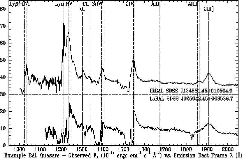
Figure 1: Rest-frame spectra of two illustrative BAL quasars from the SDSS Early Data Release quasar sample (Schneider et al. 2002). The units of $F_{\lambda}$ are $10^{-17}$ ergs cm^-2 s^-1 Å^-1 in this and all following Figures. The top spectrum is the HiBAL SDSS J124551.45+010504.9 (LBQS 1243+0121), with absorption in C iv, O vi, N v, Si iv, and Ly$\alpha$. The bottom spectrum is the LoBAL SDSS J025042.45+003536.7. Its spectral coverage does not include O vi, but all other species seen in absorption in the HiBAL are present, as well as Al iii, C ii, and possibly very weak Al ii. (The spectral coverage does not include Mg ii.) These spectra help illustrate the range of properties seen in BAL outflows. The absorption does not go to zero in either object (partial covering), though it does come close. In the HiBAL, the C iv and Si iv trough profiles are similar but not identical: both appear somewhat detached from the emission line, but C iv is deeper at the lowest outflow velocities. The weak Ly$\alpha$ absorption shows that the BAL outflow is highly ionized. In the LoBAL, the Al iii and C ii troughs are narrower and weaker than the C iv and Si iv troughs. Usually they appear weaker due to lower partial covering, but without high-resolution spectra the possibility of unsaturated low-ionization troughs cannot be ruled out. There appear to be two systems in the outflow: a narrow low-velocity system which is highly ionized (weak C ii, strong N v) and a broad high-velocity system which includes the bulk of the low-ionization absorption, accompanied by strong Ly$\alpha$ absorption. This LoBAL is slightly unusual in that respect: low-ionization absorption is usually strongest at the lowest outflow velocities.

BAL quasars are divided into three observational subtypes depending on what type of transitions are seen in absorption. A list of relevant transitions with rest frame $\lambda_{vac}$$>$1215 Å is given in Table 1, and two of these three subtypes are illustrated and discussed in Figure 1. High-ionization BAL quasars (HiBALs) show absorption from C iv, N v, Si iv, and Ly$\alpha$ (in order of decreasing typical strength, for $\lambda_{vac}$$>$1215 Å). Low-ionization BAL quasars (LoBALs; Voit, Weymann, & Korista 1993) exhibit the above high-ionization absorption plus absorption in Mg ii, Al iii, Al ii and sometimes Fe ii, Fe iii and other low-ionization species, again roughly in order of decreasing strength. Note that the absorbing gas has a range of ionization states even in HiBALs. The observed range simply extends to lower ionization states in LoBALs. The rare Iron LoBALs (FeLoBALs; Hazard et al. 1987; Cowie et al. 1994; Becker et al. 1997, 2000; Menou et al. 2001) also show absorption from excited fine-structure levels or excited atomic terms of Fe ii or Fe iii.

A key feature of BAL outflows which has only recently been appreciated is that the absorption is saturated (optical depth $\tau$ of a few) in almost all cases where optical depths can be determined using line ratios and other saturation diagnostics (e.g., Arav et al. 2001b). This is true even though the absorption troughs rarely reach zero flux. This ‘nonblack saturation’ means that the BAL outflows typically exhibit partial covering of the continuum source (Arav et al. 1999a), possibly combined with infill of the troughs by host galaxy light or scattered light which bypasses the BAL outflow (Ogle et al. 1999). The BAL outflow is usually thought to lie outside the broad emission line region since both the continuum and the broad emission lines are absorbed in most objects (Turnshek et al. 1988). However, in some cases, only the continuum emission is absorbed (Arav et al. 1999a).

Species of a given ionization tend to have similar but not identical trough shapes in velocity space, due to similar but not identical partial coverings as a function of velocity for different ions (e.g., Arav et al. 2001b). When present, low-ionization troughs are always narrower than high-ionization troughs, are usually strongest at low outflow velocities (Voit et al. 1993; but see Arav et al. 2001a), and are often seen in relatively narrow features where the high-ionization absorption is strongest. This latter feature indicates that the low and high ionization regions are closely associated (e.g., de Kool et al. 2001). Large local density gradients are probably required for gas with ionization parameter $U$ ranging at least from 10^-2 to 1 (Arav et al. 2001b) to exist in such close proximity (Arav et al. 2001a).

BAL troughs have never been seen to vary in velocity at a significant level. Limits on the acceleration reach $<$0.03 cm s^-2 in one case (Wampler, Chugai, & Petitjean 1995), and the most significant variations claimed are only $\Delta v=55\pm 25$ km s^-1 over 5 rest-frame years ($dv/dt$=0.035 cm s^-2; Vilkoviskij & Irwin 2001) and $\Delta v=125\pm 63$ km s^-1 over 6.6 rest-frame years ($dv/dt$=0.06 cm s^-2; Rupke, Veilleux, & Sanders 2002). Thus the BAL gas must either be coasting or in a stable flow pattern with a significant transverse velocity component (Arav et al. 1999b). BAL troughs have been seen to vary in strength (§6.4.1), probably due mostly to variations in covering factor rather than ionization, since BAL troughs are typically saturated with optical depths $\tau$ of a few (e.g., Arav et al. 2001b).

2.2 BAL Quasar Fraction and Global Covering Factor

BAL quasars form 8% of the optically selected flux-limited Large Bright Quasar Survey, but 11% after accounting for the average differential optical/UV $k-$correction between BAL and non-BAL quasars caused by the absorption troughs (Weymann 1997). LoBALs comprise $\sim$15% of BAL quasars (W91), but the differential $k$-correction between LoBALs and HiBALs could be substantial (Sprayberry & Foltz 1992). If all quasars can be BAL quasars when viewed along certain lines of sight, then the $k$-corrected BAL quasar fraction should be equal to the average global covering factor (GCF) of those lines of sight (Morris 1988).

The $k$-corrections used to estimate the true BAL quasar fraction must also account for any differential attenuation between BAL and non-BAL quasars. It has been widely held that HiBALs as a population are not heavily reddened (e.g., W91) but that LoBALs are (Sprayberry & Foltz 1992), and thus that the true fraction of LoBALs is underestimated by flux-limited optical surveys. Other surveys can overcome this bias: $\sim 20_{-10}^{+15}$% of all IRAS-selected quasars are LoBALs (W91; Low et al. 1989; Boroson & Meyers 1992) and $18_{-9}^{+14}$% of BAL quasars are LoBALs in the optical and radio flux-limited FIRST Bright Quasar Survey (FBQS), which has an observed BAL quasar fraction of 14$\pm$4% (18$\pm$4% if the balnicity criterion is relaxed; Becker et al. 2000). The FBQS and the SDSS also find that HiBALs as well as LoBALs are reddened (Brotherton et al. 2001b; Menou et al. 2001). Thus all types of BAL quasars are underrepresented in optical flux-limited samples and the true average GCF must be $>$0.11. A GCF of $\sim$0.3 would help explain why BAL quasars are typically more polarized than non-BAL quasars (Schmidt & Hines 1999; Hutsemékers & Lamy 2000) and have generally weaker narrow [O iii] emission (Boroson & Meyers 1992).

An upper limit to the GCF can be estimated since broad absorption line troughs are really broad scattering troughs: absorption of these resonance line photons is followed by emission of an identical photon. If the GCF was unity, then the ‘absorbed’ flux would be redistributed to a red wing in each line, and the emission and absorption equivalent widths (EW) would be identical (Hamann, Korista, & Morris 1993). Since the absorption EW is typically much greater than the emission EW, the BAL gas must have GCF$\lesssim$0.3. However, this inference ignores the very real possibility of preferential destruction of line photons by dust, particularly in LoBALs (Voit et al. 1993). At least some LoBALs meet every test for being recently (re)fueled quasars “in the act of casting off their cocoons of dust and gas” (Voit et al. 1993). Such dust, combined with near-unity GCFs, helps explain many of their unusual properties (Canalizo & Stockton 2001).

2.3 Theoretical Models

The scattering of resonance line photons can provide the radiative acceleration which at least partially drives BAL outflows (Arav et al. 1995). The difficulty arises in accelerating the gas to sufficient velocities without completely stripping the resonance-line-absorbing ions of their electrons. The disk wind model of Murray & Chiang (1998, and references therein) has been very successful in explaining this and other properties of BAL quasars. In this model, a wind from an accretion disk is shielded from soft X-rays by a high column density ($N_{H}\gtrsim 10^{23}\,\rm cm^{-2}$) of highly ionized gas ($U\sim 10$). Being stripped of many outer electrons, the ions in this ‘hitchhiking’ gas transmit UV photons from resonance lines such as C iv. Thus the wind can be accelerated by scattering such photons without becoming too highly ionized by higher energy photons. The ‘hitchhiking’ gas successfully explains the strong soft X-ray absorption in BAL quasars ($N_{H}=10^{23-24}$ cm^-2; e.g., Green et al. 2001a) and absorption from very high ionization lines (up to Ne viii, Mg x, and Si xii in SBS 1542+541; Telfer et al. 1998). The quasar structure proposed by Elvis (2000) also posits a disk wind, but from a narrow range of radii, such that BAL quasars are only observed when the line of sight is directly aligned with the wind. A recent summary of theoretical and computational modeling of disk winds can be found in Proga, Stone, & Kallman (2000). Some BAL quasars, particularly LoBALs, may be quasars cocooned by dust and gas rather than quasars with disk winds (Becker et al. 2000), but the only serious modeling relevant to this alternative has been the work of Williams, Baker, & Perry (1999).

It is clear that broad absorption line quasars remain an active area of research. Disk wind models explain many properties of BAL quasars, but it is unclear if they can explain the full range of BAL trough profiles and column densities. The average global covering factor of BAL gas and the range of global covering factors remain uncertain. Thus it is an open question how many BAL quasars are normal quasars seen along special lines of sight, and how many are young quasars emerging from dusty ‘cocoons’. BAL quasars with unusual and extreme properties may be useful in answering some of these questions.

3 SDSS Observations and Data Processing

Whenever possible, the spectral and photometric data presented here are taken from the SDSS Early Data Release (EDR), since it was produced with essentially a single uniform version of the SDSS data processing pipeline. A detailed description of the EDR observations and reductions is given by Stoughton et al. (2002). Here we review only a few points relevant to our primarily spectroscopic analysis. SDSS spectra are obtained using plates holding 640 fibers, each of which subtends 3″ on the sky, and cover 3800–9200 Å with resolution of $1800<R<2100$ and sampling of $\simeq$2.4 pixels per resolution element. The relative spectrophometric calibration is good to $\sim$10%, but the absolute spectrophometric calibration to only $\sim$30%. Many objects have spectra from multiple plates for quality assurance purposes. All spectra presented here are coadditions of all available spectra using inverse variance weighting at each pixel. Unless otherwise indicated, all spectra are from the SDSS; the exceptions are from the Keck, CFHT, and ARC 3.5m telescopes.

All magnitudes in this paper are PSF magnitudes calculated by fitting a model PSF to the image of the object and correcting the resulting magnitude to a 7$\farcs$4 aperture (Lupton et al. 2001 and §4.4.5 of Stoughton et al. 2002). The SDSS uses asinh magnitudes (Lupton, Gunn, & Szalay 1999) which differ from traditional magnitudes by $<$1% for signal-to-noise ratios SNR$\gtrsim$10. Because the photometric calibration is still uncertain at the $\sim$5% level, all magnitudes are provisional and are denoted using asterisks. The astrometric calibration is good to 0$\farcs$1 RMS per coordinate. IAU designations for each object presented here (e.g., SDSS J172341.09+555340.6) are given in the Tables, but are shortened in the text for brevity (e.g., SDSS 1723+5553). Full IAU designations given in the text refer to quasars in the EDR quasar catalog (Schneider et al. 2002).

4 BAL Quasar and Unusual BAL Quasar Selection

Visual inspections were carried out to flag unusual spectra which were not immediately identifiable as normal quasars, HiBALs, LoBALs, or any other known type of object or spectral reduction problem. SFA and/or PBH inspected all 95 spectroscopic plates in the EDR, all 43 other plates with numbers less than 416 — the highest number in the EDR — completed on or before modified julian date (MJD) 52056, and a selection of 69 ‘post-EDR’ plates numbered 417 and up. Also, all EDR spectra not targeted and spectroscopically confirmed as galaxies were inspected by DEV and/or AEB, and all EDR objects spectroscopically classified as quasars were re-inspected by PBH. Many other workers also inspected varying quantities of plates so that each spectrum has likely been inspected three times.

Most of the unusual objects found were unusual BAL quasars. From $\sim$120,000 spectra on 207 spectroscopic plates, including $\sim$8,000 quasar spectra, we have identified eighteen unusual BAL quasars and two mysterious objects which might be unusual BAL quasars (§5.5). Three additional unusual BAL quasars were selected from SDSS images but were confirmed with spectra obtained with other telescopes. All these unusual BAL quasars can be divided into a handful of categories, as discussed in the next section. We are confident that there are no further examples of these categories of unusual BAL quasars on the inspected plates among spectra which have SNR$\geq$6 per pixel in at least one of the $g$, $r$ or $i$ bands. This is the only sense in which our unusual BAL quasar sample could be considered a complete sample. A quasar sample from all the plates we inspected has not yet been defined, and the EDR quasar sample (Schneider et al. 2002) is incomplete because not all quasar candidates in the EDR area have been observed spectroscopically and because the quasar candidate selection criteria were not the same for all spectroscopic observations in the EDR. Nonetheless, since it is of interest to know what fraction of the quasar population unusual BAL quasars comprise, in §6.6 we estimate this fraction for the EDR.

Table 2 gives general information on the unusual BAL quasars presented in this paper. In particular, the Target Code shows whether or not the object was targeted by the Quasar, FIRST, ROSAT, Serendipity and star selection algorithms (see the Note to the Table, and Stoughton et al. 2002). None of our objects were selected as galaxy targets, or as ROSAT targets. Only three objects were not selected as Quasar targets, and one of them (SDSS 1730+5850) was not selected only because of its faintness. Only one target (SDSS 0127+0114) was completely overlooked by color selection and was selected only as a FIRST target.

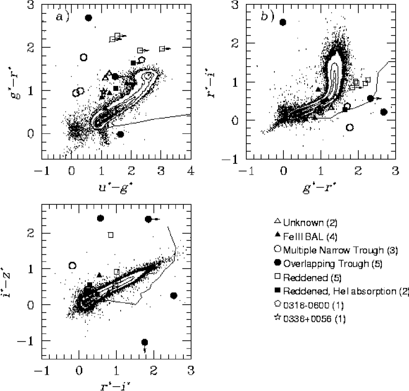
Figure 2: The distribution of unusual BAL quasars in SDSS color space. Each panel is a projection of SDSS color-color space with dots and contours showing the locus of unresolved objects (mostly stars). The line in each panel shows the mean color of simulated quasars as a function of redshift (Fan 1999), with lower redshifts to the left. Most of the change in color with redshift is due to the influence of the Ly$\alpha$ forest; for ordinary quasars with $z<2.5$, the colors are almost unchanging (see Richards et al. 2001). Thus most of the objects in the cloud with $-0.2<u^{*}-g^{*}<0.6$ and $-0.2<g^{*}-r^{*}<0.5$ are low redshift quasars. The unusual BAL quasars presented in this paper are shown with the large symbols, coded according to category as shown at the lower right, with the number of objects of each category in parentheses. Arrows denote detections at lower than 5$\sigma$ significance. Most of the quasars are at $z<2.5$, and thus most of the scatter in colors is due to the BAL troughs.

The efficiency of SDSS color selection in finding unusual BAL quasars is shown in Figure 2. The projections of the stellar locus in the three SDSS color-color diagrams are shown, along with the unusual BAL quasars presented in this paper, coded according to category. Most of the scatter in colors is due to the BAL troughs. Most of these objects have colors quite distinct from ordinary quasars as well as ordinary stars. The SDSS is sensitive to these unusual objects because the SDSS quasar target selection algorithm selects objects with unusual colors even if they lie far from the locus of ordinary quasars in color space.

All SDSS and followup spectra presented herein are available for download from the contributed data section of the SDSS Archive at http://archive.stsci.edu/sdss/. Flux densities $F_{\lambda}$ in these spectra, and in all our figures, are given in units of $10^{-17}$ ergs cm^-2 s^-1 Å^-1.

5 Categories of Unusual BAL Quasars

All of the unusual BAL quasars found in SDSS to date are LoBALs, and many are FeLoBALs. Most can be placed into one of five categories, which we now present and analyze separately. First we present three FeLoBALs with many narrow troughs (§5.1). Objects with similar numbers of troughs but higher terminal velocities could have their continua almost totally absorbed; we present five of these overlapping-trough FeLoBALs in §5.2. After that we present nine heavily reddened LoBALs (§5.3) and one slightly less reddened LoBAL with stronger Fe iii than Fe ii absorption (§5.4), along with several possibly similar objects with lower SNR. Lastly, we present two mysterious objects which may be very unusual BAL quasars (§5.5). The implications of all these objects are discussed in §6.

Absorption from many different ions is present in these objects. To identify most lines, we used the wavelengths tabulated in Moore (1962), Morton, York, & Jenkins (1988), Morton (1991) and Vanden Berk et al. (2001). Absorption and occasionally emission from many multiplets of Fe ii, Fe iii, and possibly Fe i is present in many of these objects as well. (Recall that a multiplet is the set of all transitions between two atomic terms.) To identify these lines we also used wavelengths tabulated in Moore (1950), Grandi (1981), Hazard et al. (1987) and Graham, Clowes, & Campusano (1996). These wavelengths are generally accurate enough for use with the low-resolution spectra presented here, but more accurate wavelengths are available in the Fe ii and Fe iii literature referenced by Vestergaard & Wilkes (2001).

A short word about multiplet notation is in order. The standard notation of Moore (1950) designates Fe ii multiplets either as ultraviolet (UV; $\lambda\lesssim 3000\,$Å) or optical (Opt; $\lambda\gtrsim 3000\,$Å). Both lists are ordered separately, first by increasing energy of the lower term and then by increasing energy of the upper term. Thus UV2 multiplet transitions are to a more energetic upper term than UV1, though they arise from the same lower term. The higher the multiplet number, the higher the excitation potential (EP) of its lower term (this applies to all ions, not just Fe ii). For example, Fe ii multiplets UV1 to UV9 arise from the ground term. When identifying which Fe ii multiplets are responsible for any observed absorption, we always begin with the lowest-numbered multiplet present in that wavelength range. Absorption from higher-numbered multiplets (i.e., more highly excited terms) may be present as well (or instead, if selective pumping is at work), but we prefer to be conservative in estimating the Fe ii excitation.

Where useful, BAL troughs are plotted in velocity space using

$$\beta\equiv v/c=(R^{2}-1)/(R^{2}+1){\rm~{}~{}where~{}~{}}R\equiv(1+z_{em})/(1+z_{abs})$$ (1)

(Foltz et al. 1986). The uncertainty on $\beta$ is given by

$$\sigma_{\beta}=\frac{4R^{2}}{(R^{2}+1)^{2}}\sqrt{\left(\frac{\sigma_{z_{em}}}{1+z_{em}}\right)^{2}+\left(\frac{\sigma_{z_{abs}}}{1+z_{abs}}\right)^{2}}$$ (2)

We define the zero velocity for each line using its laboratory vacuum rest wavelength.

5.1 BAL Quasars with Many Narrow Troughs

Our inspection revealed three FeLoBALs with many narrow absorption troughs, similar to FIRST 0840+3633 (Becker et al. 1997). We discuss the spectra of the high-redshift and low-redshift objects separately, and then in comparison, but defer discussion of the implications of all these objects to §6.5.

5.1.1 High Redshift Example: SDSS 1723+5553

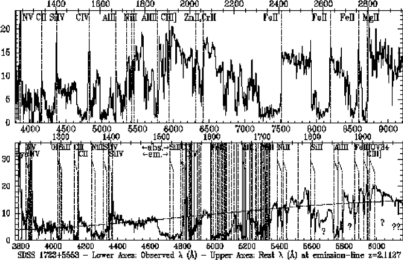
Figure 3: SDSS 1723+5553 at our adopted $z=2.1127\pm 0.0006$. The top panel shows the full spectrum and the bottom panel the spectrum shortward of 1980 Å in the rest frame. In both panels the observed wavelength is given along the bottom axis and the rest wavelength along the top axis. The units of $F_{\lambda}$ are $10^{-17}$ ergs cm^-2 s^-1 Å^-1 in this and all following Figures. In the top panel, wavelengths of notable emission and absorption features are marked with dotted lines in the adopted rest frame. In the bottom panel, dashed lines show the wavelengths of emission lines and dotted lines the wavelengths of absorption lines in the BAL outflow. Bifurcated dotted lines show absorption from the same transition in two different redshift systems. Transitions are labelled at the top of the panel; most of the transitions from 1550 Å to 1720 Å are due to Fe ii multiplets. Question marks denote absorption features of unknown origin. The smooth dot-dashed line shows the continuum fit used to calculate the BI and AI from the C iv trough. See §5.1.1 for further discussion.

This object (Figure 3) may have the most absorption troughs ever observed at this resolution in a single quasar. We identify absorption from 15 ions of 10 elements: Al ii, Al iii, C ii, C iv, Cr ii, Fe i, Fe ii, Fe iii, Mg ii, Ni ii, N v, O i, Si ii, Si iv, and Zn ii. Fe ii absorption is seen from multiplets up to at least UV79, whose lower and upper terms are 1.66 eV and 7.37 eV above ground, respectively. Only a small amount of neutral gas is probably present, since the only neutral absorption we detect is O i $\lambda$1302 (intrinsically one of the strongest neutral-atom transitions in the ultraviolet longward of Ly$\alpha$) and weak Fe i $\lambda$2484.

We adopt an emission-line redshift of $z=2.1127\pm 0.0006$ by fitting Gaussians to the apparent narrow emission lines of Si iv $\lambda$1402.77 and Mg ii $\lambda$2803.53. Both lines used to derive the redshift are the longer-wavelength lines of doublets, but the apparent emission is narrower than the doublet separations, allowing a single line to be fitted. The systematic uncertainty on our adopted redshift dwarfs the statistical uncertainty.

The bottom panel of Figure 3 shows the object’s spectrum at $\lambda<1980$ Å in the rest frame at the emission-line redshift; the spectrum at $\lambda>1980$ Å is discussed in §5.1.3. There are at least three different redshift systems in the absorbing region. The lowest redshift system has $z=2.0942\pm 0.0003$ as measured by Fe iii UV34, which is much stronger in this system than in either of the other two. The intermediate redshift system, the weakest, has $z=2.100\pm 0.001$ from Ni ii and Si ii. The highest redshift system has $z=2.1082\pm 0.0002$ from Ni ii, Si ii, Zn ii, and Cr ii; it also has weak Fe i $\lambda$2484 and probably O i $\lambda$1302. Absorption from transitions seen in both the lowest and highest redshift systems is indicated by the bifurcated dotted lines in Figure 3b. The high-ionization Si iv and C iv troughs show some features corresponding to the low-ionization redshift systems, but overall extend smoothly to outflow velocities of 11300 km s^-1.

The narrow troughs in this object enabled the identification of the absorption just longward of C iv as Fe ii UV44,45,46 absorption from terms with EP=0.15$-$0.25 eV. Such absorption has been seen before in the original FeLoBAL Q 0059$-$2735 (Wampler et al. 1995), but is much stronger here.

5.1.2 Low Redshift Examples: SDSS 1125+0029 and SDSS 1128+0113

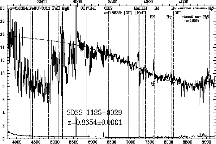
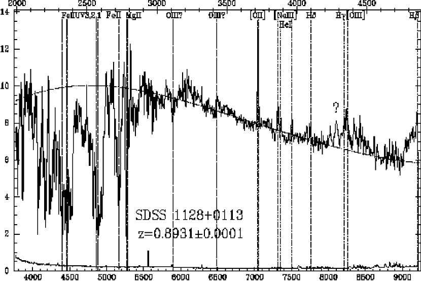
Figure 4: SDSS spectra and error arrays of a) SDSS 1125+0029 and b) SDSS 1128+0113 (Observed $F_{\lambda}$ vs. rest frame $\lambda$ in Å at the top and observed frame $\lambda$ at the bottom). All spectra and error arrays (lower curves) have been smoothed by a 5-pixel boxcar filter. The dot-dashed lines show the continuum fits used to calculate the BI and AI (Appendix A). Dotted vertical lines show the wavelengths of emission lines and dashed vertical lines show the wavelengths of absorption lines. Between 2300$-$2600 Å rest frame, the strongest lines of Fe ii multiplets UV1, UV2, and UV3 have been marked, but each is surrounded by many unmarked Fe ii lines. Most of the absorption at $\lambda_{rest}<3500$ Å can be identified with Fe ii, but the only other Fe ii absorption specifically marked is from UV62,63 at 2750 Å. In both objects Mg ii absorption is plotted at the systemic redshift, but the Mg ii trough extends longward of this redshift. See §5.1.2 for further discussion.

Figure 4 shows the full SDSS spectra of both low redshift BAL quasars with many narrow troughs.

SDSS 1125+0029

This object has narrow [O ii] $\lambda\lambda$3727,3729 emission at $z=0.8635\pm 0.0008$, in excellent agreement with the peak of the broader [Ne iii] $\lambda$3869 emission. Broad emission is visible in H$\gamma$ and H$\beta$, at $z=0.859\pm 0.002$ (possibly affected by superimposed absorption); the apparent broad emission at 7600$-$7640 Å (marked $\earth$ in Figure 4a) is just poorly removed telluric absorption. Visible in the red half of the spectrum are relatively narrow absorption lines from He i $\lambda$3889+H8, Ca ii $\lambda$3934 (K), H$\epsilon$+Ca ii $\lambda$3969 (H) blended with [Ne iii] $\lambda$3969 emission, H$\delta$, H$\gamma$, and H$\beta$. All of these lines except Ca ii K show reversed profiles: narrow emission in the center of a broader absorption trough. These narrow Balmer emission lines give $z=0.8654\pm 0.0001$, which we adopt as the systemic redshift. This is in excellent agreement with the Ca ii K redshift and agrees with the Ca ii H redshift within the errors due to blending with He i. Thus the [O ii] and [Ne iii] emission lines are blueshifted by 310$\pm$130 km s^-1 and the broad Balmer lines by 1030$\pm$320 km s^-1. The BAL outflow might contribute to the Ca ii absorption (cf. §5.2), but if the Ca ii is due to starlight it implies a host galaxy with $M_{i^{*}}\sim-24.5$, which is extremely luminous.

This object has broad emission in H$\beta$ but not in Mg ii. This could be due to preferential destruction of Mg ii line photons by dust, since resonant scattering can greatly increase the path length for line photons (Voit et al. 1993). BAL troughs present in this object include Mg ii and possibly O iii $\lambda$3133 and He i $\lambda$3188. The vast majority of the remaining absorption at $2050<\lambda_{rest}<3500$ Å is from Fe ii.

SDSS 1128+0113

This object has $z=0.8931\pm 0.0001$ as measured by narrow [O ii] $\lambda\lambda$3727,3729 emission and somewhat broader [Ne iii] $\lambda$3869, He i $\lambda$3889.74 and [Ne iii] $\lambda$3969. H$\gamma$ is present and may be slightly redshifted, but the SNR is low and it may be blended with [O iii] $\lambda$4363. H$\beta$ is also present, but we cannot determine its peak observed wavelength with any certainty since it is at the extreme red end of our spectrum. We cannot identify the apparent moderately broad emission line just shortward of H$\gamma$, at 4295 Å (marked ? in Figure 4b); there should be other lines present if it is Fe ii emission. The BAL troughs in this object are not quite as omnipresent as those in SDSS 1125+0029.

5.1.3 Comparison of Many-Narrow-Trough BAL Quasars

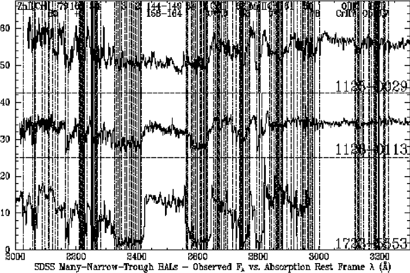
Figure 5: The spectral region near Mg ii in the three BAL quasars with many narrow troughs discussed in §5.1.3. SDSS 1125+0029 has been smoothed by a 3-pixel boxcar filter, while unsmoothed spectra are displayed for the other two objects. Horizontal dashed lines show the zero flux levels for the top two spectra. Each spectrum is plotted in the rest frame of its deepest absorption trough, and dotted vertical lines show the wavelengths of selected absorption lines in this frame. Dashed vertical lines show the wavelengths of Mg ii $\lambda\lambda$2796,2803, O iii $\lambda$3133 and He i $\lambda$3188 in the adopted systemic rest frame of each object (see text). This shows that in the top two (lower-$z$) objects, the Mg ii trough extends longward of the systemic redshift. Absorption complexes are labelled just to the left of the longest wavelength transition in the complex whenever possible. Optical Fe ii multiplets are labelled Opt#, while UV Fe ii multiplets are labelled just by number; for clarity, lines for multiplets 144$-$149 and 158$-$164 near 2500 Å are not plotted. Not every absorption line matches an obvious feature because the lines are not all equally strong. Finally, in SDSS 1723+5553 (bottom), there is a second absorption system at a redshift between that used for the plot and the slightly higher emission redshift (best seen in Zn ii 2026 Å, at the far left). Fe ii UV2 and UV1 multiplets from this system explain the long-wavelength ends of the absorption troughs near 2400 Å and 2600 Å.

The similarity of our many-narrow-trough BAL quasars to each other is shown in Figure 5, where we plot the wavelength range 2000—3300 Å in the rest frame of the deepest absorption trough for each object. Dotted vertical lines show the wavelengths of the labelled absorption lines or numbered Fe ii multiplets in this frame. There is no sign of Mg i $\lambda$2852 absorption in any of the objects. Dashed vertical lines show the wavelengths of Mg ii $\lambda\lambda$2796,2803, He i $\lambda$3188, and two O iii transitions (see next paragraph) in the adopted systemic rest frame of each object. Note that if they are present, He i $\lambda$3188 is blended with Fe ii Opt6 and Opt7 and the weaker He i $\lambda$2945 line, is blended with Fe ii UV60 and UV78. No absorption trough reaches zero flux in any object, indicating partial coverage of the continuum source by the absorbing region, and possibly a contribution from scattered light which bypasses the absorbing region. SDSS 1125+0029 (top) has the lowest partial covering but the highest Fe ii excitation, since it shows absorption which arises only from highly excited Fe ii, seen longward of Mg ii and between the more common lower excitation Fe ii absorption troughs at 2400 Å and 2600 Å (Moore 1950).

Most troughs can be identified with Fe ii multiplets, but some have uncertain identifications, notably:
$\bullet$ We initially identified the $\sim$3100-3135 Å trough with O iii $\lambda$3133, which was first identified as a BAL in CNOC2 J022509.6+001904 (Hall et al. 2000). This transition has a lower state 36.9 eV above ground, but can be indirectly populated via Bowen resonance-fluorescence with He ii Ly$\alpha$ (section 4.7 of Osterbrock 1989). However, in this case we should see O iii $\lambda$3445 with $\sim$30% the strength of O iii $\lambda$3133. Such absorption is not present in either object in Figure 4, so O iii $\lambda$3133 absorption can at best explain only part of their $\sim$3100-3135 Å troughs. The lowest-numbered Fe ii multiplet which matches this trough is Opt82 (EP 3.87 eV), but if that identification were correct we should also see absorption near 2150 Å from multiplet UV213 (EP 3.14-3.22 eV). Another possibility is Cr ii absorption from terms $\sim$2.45 eV above ground (de Kool et al. 2002), but in SDSS 1125+0029 such absorption would be improbably strong relative to the ground-term Cr ii trough at $\sim$2060 Å. Thus the origin of the $\sim$3100-3135 Å trough remains unclear.
$\bullet$ Explaining the $\sim$2220 Å trough as Fe ii requires absorption from at least UV168 (lower term EP 2.62$-$2.68 eV). The 2400$-$2550 Å absorption can then be attributed to UV144$-$149,158$-$164. Such absorption is weak in SDSS 1128+0113 and absent in SDSS 1723+5553, however, so their 2220 Å troughs are unlikely to be due solely to Fe ii UV168. A contribution from Ni ii (Table 1) is a poor fit, and Si i and Mn i can be ruled out because many other lines from neutral atoms would also be seen and are not.
$\bullet$ The strong absorption near $\sim$2665 Å may require more than just Cr ii UV7,8 to explain it.
The first two cases above might be explained by selective pumping of the lower terms of multiplets Opt82 and UV168, respectively, a possibility which can only be tested via detailed modeling of Fe ii.

5.1.4 Redshifted Absorption Troughs

The most interesting feature of both low-redshift objects presented in §5.1.2 is that the broad Mg ii doublet absorption trough extends longward of the systemic redshift (dashed vertical lines in Figure 5). In SDSS 1128+0113, the Mg ii absorption appears split into two components, but this structure may be some combination of narrow Mg ii emission and partial covering which varies with velocity.

The presence of longward-of-systemic broad absorption is quite surprising, since the absorption in BAL quasars has always previously been seen in outflow. A search for BAL troughs longward of the systemic redshift in all BAL quasars in the EDR (§6.6) turned up several additional candidates, but none stood up to scrutiny. SDSS J115852.87$-$004302.0 has $z=0.9833\pm 0.0010$ from narrow [O ii] $\lambda\lambda$3727,3729 emission. Mg ii absorption extending slightly longward of this $z$ cannot be ruled out due to noise from the 5577 Å night sky line, but there is no evidence of longward-of-systemic absorption from other lines. SDSS J131637.27$-$003636.0 has $z=0.930\pm 0.001$ from narrow [O ii] emission. There is weak Mg ii emission in the middle of what appears to be an absorption trough but is actually just a gap between emission from Fe ii multiplets. SDSS J235238.09+010552.4 has C iv absorption longward of the peak of C iv emission, but only because the C iv peak is blueshifted $\sim$4000 km s^-1 from the C iii] and Mg ii redshift of $z=2.156$.

We discuss the implications of longward-of-systemic absorption in §6.5.

5.2 BAL Quasars with Overlapping Troughs

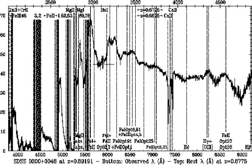
Figure 6: SDSS 0300+0048, an overlapping-trough FeLoBAL at $z=0.89191\pm 0.00005$. This assumed systemic redshift is taken from the associated Mg ii system, but accurately predicts the wavelengths of broad emission features longward of Mg ii (dashed lines are features at this redshift, labelled along the bottom of the plot). The onset of broad Mg ii absorption is at $z=0.8775$, coincident with the highest redshift Ca ii system (dot-dashed lines show absorption at this redshift, labelled along the top of the plot). However, the onset of Fe ii absorption from various UV multiplets is at $z=0.8675$, coincident with the lowest redshift Ca ii system (features at this redshift are denoted by dotted lines and the second row of labels across the top). The horizontal dot-dashed line segment shows the continuum level adopted for calculation of the AI and BI.

Several FeLoBALs have been discovered from the SDSS with abrupt drops in flux near Mg ii $\lambda\lambda$2796,2803 caused by overlapping absorption troughs. That is, the troughs remain deep at velocities comparable to the spacing of absorption troughs from different transitions, so that there are no continuum windows between the troughs (Figures 6$-$9). Troughs 19000 km s^-1 wide may be required, so that Mg ii overlaps Fe ii UV1 at $\lambda$$\leq$2632 Å; however, a width of only 13000 km s^-1 is needed if Fe ii UV62,63 absorption is present. These ‘overlapping-trough’ BAL quasars resemble Mrk 231 (Smith et al. 1995), FIRST 1556+3517 (Becker et al. 1997) and especially FBQS 1408+3054 (White et al. 2000; Becker et al. 2000), including the complex emission and absorption near Mg ii and the strong Mg i $\lambda$2852 absorption. However, the BAL region in our overlapping-trough objects covers the emission region almost totally, instead of only partially as in FBQS 1408+3054 or Mrk 231. (The spectrum of FBQS 1408+3054 can be seen in §6.1.2).

We first discuss the rest frame features common to all these objects (Figures 6$-$9), and then present them individually, in order of increasing redshift.

The apparent emission lines shortward of Mg ii are identified as regions near the high-velocity (blue) ends of various absorption troughs. At high outflow velocities, the partial covering of the absorption, or possibly its optical depth, typically decreases so that the observed flux begins to recover to the continuum level. The troughs are broad enough, however, that before this recovery is complete, another absorption trough is encountered and the observed flux drops abruptly. These abortive recoveries toward the continuum level can mimic the appearance of broad emission lines.

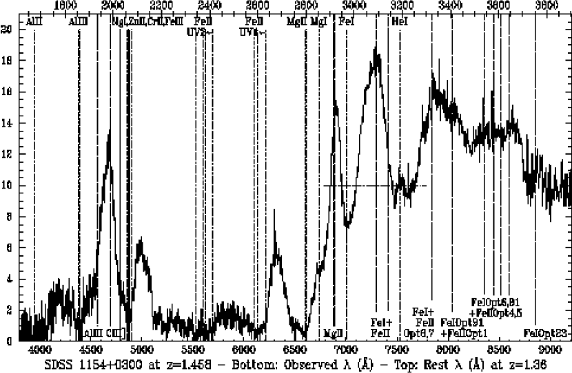
Figure 7: SDSS 1154+0300, an overlapping-trough FeLoBAL at $z=1.458\pm 0.008$. Dashed lines labelled along the bottom of the plot show emission features at this redshift, while absorption features at the redshift of peak absorption ($z=1.36$) are labelled along the top of the plot. Only the ground level lines and longest-wavelength excited level lines are plotted for Fe ii multiplets UV1 and UV2. The horizontal dot-dashed line segment shows the continuum level adopted for calculation of the AI and BI.

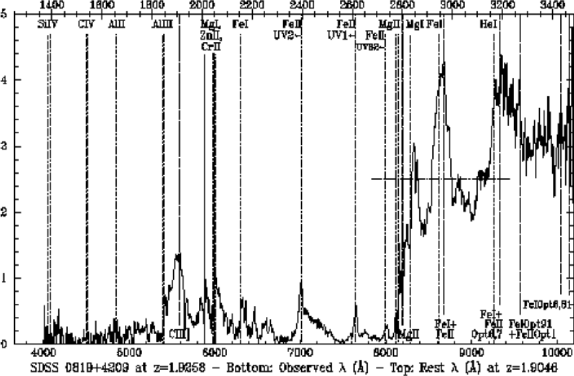
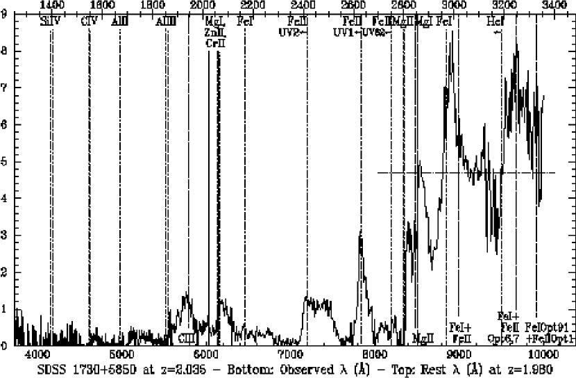
Figure 8: Two high redshift overlapping-trough FeLoBAL quasars. In each plot, dashed lines show emission features at the systemic redshift, labelled along the bottom of the plot. Dotted lines show absorption features at the redshift of the red edge of the Mg ii trough, labelled along the top of the plot. Only the longest-wavelength lines are plotted for Fe ii multiplets UV1, UV2, and UV62. In each plot, the horizontal dot-dashed line segment shows the continuum level adopted for calculation of the AI and BI. a) SDSS 0819+4209 at $z=1.9258\pm 0.0006$. This assumed systemic redshift is taken from associated Mg i and Mg ii, but accurately predicts the wavelengths of various broad emission features. The redshift of the long-wavelength edge of the Mg ii trough is $z=1.9046\pm 0.0005$. Only the longest-wavelength lines are plotted for Fe ii multiplets UV1, UV2, and UV62. b) SDSS 1730+5850 at $z=2.035\pm 0.005$. This assumed systemic redshift is taken from C iii] $\lambda$1908 and He i $\lambda$3188 emission. There may be extensive He i $\lambda$3188 absorption starting at a redshift just below $z=1.980\pm 0.005$ (the latter is the onset redshift of the Mg ii trough).

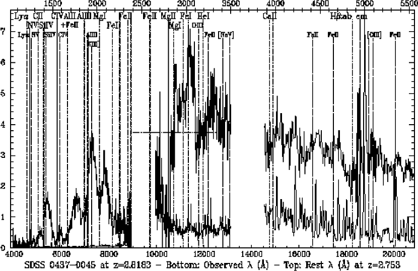
Figure 9: Optical (Keck) plus NIR (UKIRT) spectra and error arrays of SDSS 0437$-$0045 at $z=2.8183\pm 0.0009$. The top two rows of labels show the wavelengths of absorption lines at the redshift of peak absorption, $z=2.753$. Below that, emission lines are shown at the adopted systemic redshift. There is no evidence for [O iii] emission at $z=2.8183$, but we plot its wavelengths for reference. Note the nearly complete absorption from Fe ii near the expected wavelength of C iv, and the possible broad H$\beta$ absorption. (The apparent emission feature at 5000 Å in the $z=2.753$ frame is a sky line residual; note the peak in the error spectrum just below it.) The horizontal dot-dashed line shows the continuum level used in calculating the AI and BI.

Longward of Mg ii, the spectra are mostly free from absorption and we can identify emission features by comparison to the SDSS composite quasar spectrum (Vanden Berk et al. 2001), allowing for emission from strong Fe i and Fe ii multiplets whose lower terms are $\lesssim$3 eV above ground. In our object with the best coverage longward of Mg ii (Figure 6), we see H$\beta$ in emission, Fe ii Opt37,38 at 4570 Å, H$\gamma$+[O iii] at 4350 Å, Fe i Opt5,21 at 3735 Å, Fe i Opt23 emission at 3600 Å, a feature at 3350$-$3550 Å including Fe i Opt6,81 at 3465,3435 Å and possibly Fe ii Opt4,5 at 3500,3400 Å, a feature at 3150$-$3300 Å including Fe i Opt91+Fe ii Opt1 at 3280 Å and He i+Fe ii Opt6,7+Fe i Opt155-158 at 3200 Å, and a blend of Fe i Opt9,30 at 3015 Å with Fe ii UV60,78+Fe i UV1 at 2970 Å. Many of these features are also visible in Figures 7-9.

Near Mg ii the spectra are blends of emission and absorption. There may be He i, Fe i and/or Fe ii absorption shortward of the 3200 Å emission feature in some or all of the objects, most notably in SDSS 1730+5850 (Figure 8b). There is almost certainly Fe i and/or Fe ii absorption shortward of the 2970 Å emission feature, because the observed flux dips lower than essentially any point in the continuum longward of Mg ii. Dust may contribute to this drop in flux, but the effect is too sudden to be entirely due to dust. Also, in all objects except SDSS 0819+4209 (Figure 8a), the flux recovers to this level at least once shortward of Mg ii, which would not be the case if dust reddening were already affecting the spectrum strongly at 3000 Å. Mg ii $\lambda\lambda$2796,2803 emission must also contribute to the spectrum in this region, but Mg i $\lambda$2852 and Mg ii absorption are so strong and abrupt that only a narrow sliver of probable Mg ii emission remains, just longward of the onset of those troughs.

Shortward of Mg ii, the overlapping troughs make detailed line identifications quite difficult. However, we know that these objects are FeLoBALs because they show Fe ii UV62,63 absorption at 2750 Å (e.g., Figure 6) and because they show Fe ii* UV1 absorption. The latter can be identified because absorption from excited levels in the UV1 multiplet extends to 2632 Å, while ground level UV1 absorption extends only to 2600 Å. Given low-ionization troughs 13,000$-$19,000 km s^-1 wide or wider, Fe ii absorption can blanket the spectrum down to at least 2100 Å. A recovery of flux is detectable in all these objects around the C iii] $\lambda$1908 line, from 2100 Å down to the onset of Al iii absorption at 1860 Å. Al iii blended with Fe ii and other low-ionization lines (cf. Figure 3) can overlap with Al ii and still more Fe ii all the way down to C iv. Then, given that high ionization troughs are typically broader than low ionization troughs, it is not surprising that the C iv trough overlaps with Si iv and Si iv with N v, so that the entire spectrum down to Ly$\alpha$ is essentially extinguished.

We assume the continuum in these objects shortward of Mg ii is flat in $F_{\lambda}$ at the level of the 3100 Å window (indicated by a short dot-dashed line in each Figure). This window may be affected by absorption from He i $\lambda$3188, Fe ii or even O iii $\lambda$3133, as well as by reddening, but in the three objects with significant coverage longward of it, this window is not a bad match to the continuum. We use 19000 km s^-1 as the upper velocity limit when calculating the AI and BI from Mg ii in most of these objects (Appendix A). The maximum AI in that case is 19000 km s^-1, while the maximum BI depends on the detachment velocity of the BAL trough. For SDSS 0437$-$0045, we use C iv to measure the AI and BI (maximum values 25000 km s^-1 and 20000 km s^-1  respectively) since our spectra fully cover the C iv region in that object.

5.2.1 SDSS 0300+0048

In addition to an extremely broad Mg ii BAL trough, SDSS 0300+0048 (Figure 6) shows a strong Ca ii H&K BAL trough. This Ca ii absorption appears split into two relatively narrow systems, at $z=0.8675$ and $z=0.8775$ ($\Delta v$=1550 km s^-1), although there is also broad Ca ii absorption extending a further 2000 km s^-1 shortward. There is associated Mg ii and Mg i $\lambda$2852 absorption 2300 km s^-1 longward of the highest redshift Ca ii system, at $z=0.89191\pm 0.00005$. We have adopted this latter value as the systemic redshift. Associated narrow Mg ii systems with $z_{abs}>z_{em}$ do exist, but 2300 km s^-1 would be an extreme velocity for such a system (Foltz et al. 1986), whereas BAL troughs detached by 2300 km s^-1 shortward of $z_{em}$ are unremarkable. Ca ii H&K absorption in BAL outflows has been seen before only in the Seyfert 1/LoBAL Mrk 231 (Boksenberg et al. 1977) and the FeLoBALs FBQS 1044+3656 (White et al. 2000) and Q 2359$-$1241 (Arav et al. 2001a). SDSS 0300+0048 is also a FeLoBAL, with Fe ii absorption at 2750 Å and near 2400 and 2600 Å. However, the Fe ii BAL trough is associated only with the $z=0.8675$ Ca ii system ($v=3900$ km s^-1), while the Mg ii BAL trough begins at $z=0.8775$, the redshift of the other Ca ii system ($v=2300$ km s^-1).

Note that SDSS 0300+0048 is a binary quasar with SDSS J025959.69+004813.5, a non-BAL quasar located 19$\farcs$5 away at $z=0.894\pm 0.001$ ($\Delta v=330\pm 160$ km s^-1).

5.2.2 SDSS 1154+0300

The smooth troughs in SDSS 1154+0300 (Figure 7) make its redshift difficult to pin down. We adopt $z=1.458\pm 0.008$ from various emission features. The absorption probably begins at this redshift (e.g., in Al iii $\lambda\lambda$1854,1862), but does not reach its full depth until $z=1.36$. Rest wavelengths at the latter redshift are plotted along the top axis of Figure 7. The more rapid onset of absorption in Al iii compared to Mg ii suggests that the BAL region may cover the Al iii broad line region but not the Mg ii broad line region.

5.2.3 SDSS 0819+4209

SDSS 0819+4209 (Figure 8a) was discovered in a search for $z\gtrsim 5.8$ quasars among $i$-dropouts in SDSS images (Fan et al. 2001). The sharp drop due to Mg ii absorption mimicks the onset of the Ly$\alpha$ forest at high redshift. The spectrum was obtained with ESI (Epps & Miller 1998) at Keck II on UT 19 Mar 2001. We adopt $z=1.9258\pm 0.0006$ from unresolved Mg i absorption, accompanied by broader Mg ii absorption, located 2180$\pm$80 km s^-1 longward of the onset of the absorption troughs at $z=1.9046\pm 0.0005$.

5.2.4 SDSS 1730+5850

SDSS 1730+5850 (Figure 8b) has $z=2.035\pm 0.005$ and shows no flux, within the errors, below Al ii $\lambda$1670. It may have very extensive He i $\lambda$3188 absorption starting just shortward of $z=1.980\pm 0.005$, the onset redshift of the Mg ii and Mg i BAL troughs, though this needs confirmation given the strong telluric absorption at those observed wavelengths. This object was discovered using the Double Imaging Spectrograph (DIS) at the APO 3.5m on UT 27 May 2000 during exploratory spectroscopy of SDSS objects with odd colors. Spectra were later obtained twice by the SDSS, on UT 23 Aug 2000 and 18 Apr 2001. No significant variability was detected between those observations (not surprising given the low SNR of the spectra). The coadded SDSS spectrum is a factor of $\sim$2.25 fainter than the discovery spectrum. This discrepancy, while large, could be due to the uncertainties in the SDSS fluxing and in comparing slit and fiber spectra. The scaled SDSS spectrum shows good agreement with the discovery spectrum at $\lambda_{rest}>2600$ Å, but the ‘peaks’ at 1900 Å, 2100 Å and 2500 Å are stronger by a factor of 1.4–2. That is, the absorption at those wavelengths appears weaker than in the discovery spectrum. Nonetheless, the uncertainties are so large that we do not feel this is a firm detection of variability, though it does suggest that careful monitoring of this object might be worthwhile. In Figure 8 we have therefore summed the scaled discovery spectrum and the coadded, smoothed SDSS spectrum to achieve the best SNR and wavelength coverage.

5.2.5 SDSS 0437$-$0045

SDSS 0437$-$0045 was selected from early SDSS images by XF and MAS as having unusual colors (Fan et al. 1999). Optical spectra were obtained at the APO 3.5m using DIS on UT 22 Mar 1999, 29 Dec 1999, and 04 Jan 2000, at Keck II using the Low Resolution Imaging Spectrograph (LRIS; Oke et al. 1995) on UT 15 Oct 1999, and at the Canada-France-Hawaii Telescope (CFHT) using the Subarcsecond Imaging Spectrograph (SIS; Crampton et al. 1992) on UT 27 Jan 2001. Standard IRAF reduction procedures were used to obtain flux-calibrated spectra. Near infrared spectra covering 1.45-2.09 $\mu$m at resolution 0.0025 $\mu$m and 1.0-1.32 $\mu$m at resolution 0.0050 $\mu$m were obtained using the Cooled Grating Spectrometer (CGS4; Mountain et al. 1990) at the United Kingdom Infrared Telescope (UKIRT) on UT 27 and 30 Sep 1999 respectively. The longer wavelength spectrum was obtained under non-photometric conditions. The data were reduced using the Starlink Figaro package. Near-IR (NIR) photometry obtained by HWR at Calar Alto in Nov. 1999 yields $J=17.2$, $H=16.7$ and $K=16.2$, making $J-K$ somewhat bluer than average for a quasar. The spectra at 1.1-1.312 µm and 1.5-1.75 µm were normalized to the fluxes expected from the $J$ and $H$ photometry, respectively. A further correction of 1.33 was applied to the longer-wavelength spectrum to make the spectral slope continuous between $J$ and $H$. The true slope is probably bluer than shown, since the more trustworthy photometry indicates the object is bluer than the the long-wavelength spectrum is.

Figure 9 shows the combined optical (Keck) and NIR (UKIRT) spectrum of SDSS 0437$-$0045, which finally enabled us to identify the object after being stumped by it for some time. It is a strongly absorbed quasar with troughs that reach peak depth at $z=2.753\pm 0.002$. There is evidence for Al iii absorption at $z=2.8183\pm 0.0009$. Since the lack of abrupt long-wavelength edges to the absorption troughs in the optical suggests that the systemic $z$ is higher than the peak absorption $z$, we adopt $z=2.8183\pm 0.0009$ as our systemic redshift. In Figure 9 we plot emission lines at this redshift and absorption lines at the peak absorption redshift. There seems to be considerable absorption from neutral gas, namely several Fe i lines, Mg i $\lambda$2852, and Mg i $\lambda$2026, the latter possibly blended with Zn ii. There is no evidence for Ca ii absorption, but we plot its wavelengths for reference. As for emission, C iv appears absent because it is completely eaten away by Fe ii multiplets UV44,45,46. Note that the lines we identified as [O iii] at $z=2.74389$ in Hall et al. (2001) are at the wavelengths of night sky lines, and are almost certainly not real.

This object may have H$\beta$ absorption nearly 10⁴ km s^-1 wide, with rest-frame EW$\sim$100 Å. H$\beta$ absorption in AGN has previously been seen only in NGC 4151 (Anderson & Kraft 1969; Sergeev et al. 1999), and there with $\leq$1000 km s^-1 width and $\leq$3 Å rest-frame EW. However, the SNR is not high enough to be sure this dip in the continuum is real. Even if so, it may just be a gap between H$\beta$ and Fe ii Opt37,38 emission (e.g., Figure 4 of Lipari 1994; see also the spectrum of FBQS 1408+3054 in §6.1.2). The expected wavelengths of emission from this and three other strong Fe ii emission multiplets are plotted in Figure 9. The features $\sim$75 Å to the red of each of them argue that SDSS 0437$-$0045 has strong Fe ii emission at a slightly higher systemic redshift than we have assumed, and not an H$\beta$ BAL trough. A better spectrum is needed.

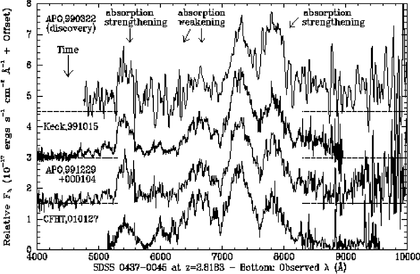
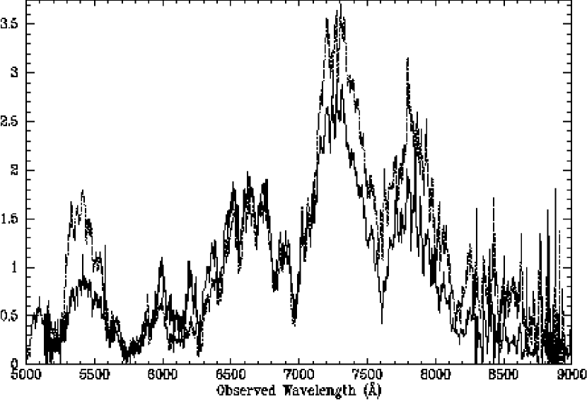
Figure 10: a) Optical spectra of SDSS 0437$-$0045 at four epochs, with time increasing downwards. All spectra have been normalized relative to the flux in the CFHT spectrum at 7000$-$7600 Å. The upper 3 spectra have been offset by +1.5 units in $F_{\lambda}$ from each other; the dashed lines show the zero flux levels. The APO discovery spectrum has been smoothed by a 5-pixel boxcar and the CFHT spectrum by a 3-pixel boxcar. The labels note the behavior of the absorption with time in the regions of the spectrum indicated, relative to the absorption in the 7000$-$7600 Å region. b) The Keck spectrum (dotted line) compared to the 3-pixel-smoothed CFHT spectrum (solid line), with no mutual normalization applied. This demonstrates the typical absolute flux calibration uncertainties among our spectra, which prevent us from determining at exactly which wavelengths the absorption has varied. However, it is still clear that relative to the absorption at 7000$-$7600 Å, the absorption at 5400 Å strengthened and that at 5900$-$7000 Å weakened between the epochs of the Keck and CFHT spectra. Only $\sim$90 rest-frame days separate the two epochs.

The absorption shortward of 2500 Å in this object has varied with an unusually high amplitude and rate of change for BAL quasars. Figure 10a shows the optical spectrum of SDSS 0437$-$0045 at four different epochs. The spectra have been normalized at 7000$-$7590 Å, where the SNR is highest, to match the CFHT spectrum. For reference, Figure 10b compares the CFHT and Keck spectra without normalization, illustrating the typical variation in absolute flux among our spectra. Our normalization accounts for the uncertainty in the absolute flux calibration of these narrow slit observations. The relative wavelength-dependent flux calibrations are trustworthy; for example, the normalized Keck and second-epoch APO spectra, taken within 20 rest-frame days of each other, agree completely within the errors across the wavelength range 4500$-$9000 Å. This also reassures us that the variability is not due to fluctuations in system sensitivities or flatfields.

To calculate the variation of the absorption strength in SDSS 0437$-$0045, we assume the true continuum is flat in $F_{\lambda}$ at $5\times 10^{-17}$ ergs cm^-2 s^-1 Å^-1. Then, relative to the 7000$-$7590 Å region, in the 90 rest-frame days between the Keck and CFHT spectra epochs the absorption weakened by 5$\pm$1% at 5200$-$5600 Å (high-velocity C iv) and strengthened by 8$\pm$1% at 5900$-$7000 Å (where narrow troughs of Fe ii, Al ii and Al iii are visible) and 5$\pm$2.5% at 7590$-$8150 Å (Mg i and Fe ii, plus Zn ii, Cr ii and Fe iii?). This last spectral region contains the strong telluric O₂ absorption band at 7590$-$7700 Å, but the increase in absorption is larger than the telluric correction applied and the region of apparently increased absorption is wider than the absorption band. This increase in the relative absorption at 7590$-$8150 Å is somewhat less than the 15$\pm$3% increase in this region in the 54 rest-frame days between the discovery and Keck spectra (Figure 10a).

The variable absorption in SDSS 0437$-$0045 is discussed further in §6.4.1.

5.3 Heavily Reddened BAL Quasars

SDSS has discovered a number of heavily reddened BAL quasars. After a short discussion of how we determine the reddening in these objects, we present two reddened mini-BALs with strong Fe ii emission, then several extremely reddened objects with no strong emission, and finally a bright reddened FeLoBAL. The implications of all these objects are discussed in §6.3.

5.3.1 Estimating the Reddening

Since the ‘typical’ quasar has a very blue spectrum, reddened quasars are easy to identify. Determining the amount of reddening is more difficult. We assume all reddening occurs at the quasar redshift with a Small Magellanic Cloud (SMC) extinction curve (Prevot et al. 1984) and $R_{V}=3.1$ (see below). We deredden the spectrum until the continuum slope matches that of the composite SDSS quasar of Vanden Berk et al. (2001). The value of the color excess $E(B-V)$ needed to achieve this match is our estimated reddening. The uncertainties on $E(B-V)$ for each object denote the range for which an acceptable match can be found.

We use the SMC extinction curve because the 2200 Å bump present in the LMC and Milky Way extinction curves has never been detected from dust around quasars (e.g., Pitman, Clayton, & Gordon 2000), although it has been detected from dust in intervening Mg ii systems (Malhotra 1997; Cohen et al. 1999). The SMC curve was also used by Sprayberry & Foltz (1992) and Brotherton et al. (2001b), both of whom found $E(B-V)$=0.1 for a ‘typical’ LoBAL spectrum. The other commonly used extinction curve is the Calzetti formula (Calzetti, Kinney, & Storchi-Bergmann 1994). This formula was derived for active star formation regions and empirically incorporates the ‘selective attenuation’ effects of dust, including extinction, scattering, and geometrical dust distribution effects. The Calzetti extinction curve does not have a 2200 Å bump, but like the LMC and MW curves it is much greyer (less steep) than the SMC extinction curve. Our use of the SMC curve instead of the Calzetti curve is conservative in the sense that it requires a lower $E(B-V)$ (and thus lower extinction) for a given observed ultraviolet slope.

Two more caveats to our dereddening procedure are needed. First, we assume a single value of $E(B-V)$ over all sightlines to the emission regions. A range of $E(B-V)$ (e.g., Hines & Wills 1995) or a wavelength-dependent contribution from scattered light (Brotherton et al. 2001a) will complicate the interpretation of our derived single $E(B-V)$. However, sometimes we can tell when these effects are important (e.g., SDSS 0342+0045; see below). Second, if an accretion disk is producing the observed emission and the amount of extinction is correlated with the inclination of the disk, then dereddening to match the SDSS composite will introduce a systematic error in the derived $E(B-V)$ since the intrinsic continuum of the disk is likely to be a function of viewing angle (e.g., Hubeny et al. 2000).

5.3.2 Two Reddened Strong Fe ii-emitting Mini-BAL Quasars

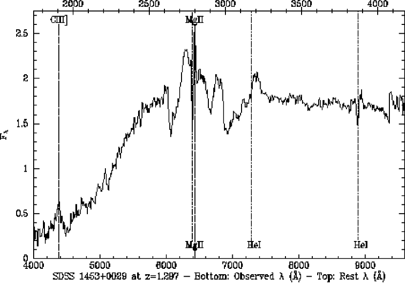
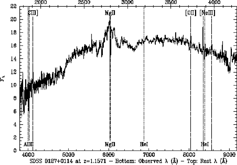
Figure 11: a) SDSS 1453+0029, a reddened extreme Fe ii-emitting mini-LoBAL quasar at $z=1.297$. b) SDSS 0127+0114, a reddened strong Fe ii-emitting mini-LoBAL quasar at $z=1.1571$. In both plots, dashed lines denote emission, and dotted lines absorption. The absorption lines are identified along the bottom of each plot and the emission lines along the top.

SDSS 1453$+$0029 was identified by XF and MAS as having unusual colors in early SDSS imaging (Fan et al. 1999). A discovery spectrum was obtained at the APO 3.5m, and a 1200s followup spectrum at Keck II on UT 05 Apr 2000 (Figure 11a). The object was observed numerous times as a quasar candidate in the SDSS spectroscopic survey. We adopt the redshift $z=1.297\pm 0.001$ determined by the pipeline from one of these observations (the other yielded no redshift), since it agrees well with the Keck spectrum.

The redshift comes from narrow Mg ii emission and weak C iii] emission. The object is similar to Q 2359$-$1241 (Brotherton et al. 2001a); both are reddened quasars with narrow Mg ii emission and absorption atop a complex broader structure. Both objects also show He i $\lambda$3188 and He i $\lambda$3889 in absorption (Arav et al. 2001a). SDSS 1453+0029 has BI=0, but AI(Mg ii)=253$-$477 km s^-1 (the lower value is from the Keck spectrum and the higher value from the coadded SDSS spectrum), with $v_{max}=1940-2210$ km s^-1.

A similar object is SDSS 0127+0114, which has Al iii, Mg ii, He i $\lambda$3188 and He i $\lambda$3889 absorption and narrow C iii], [O ii] and [Ne iii] emission, as well as broader Mg ii emission, at $z=1.1571\pm 0.0002$ (Figure 11b). SDSS 0127+0114 has zero balnicity, but the presence of He i argues that the absorption is a mini-BAL trough and not simply an associated narrow absorption line system.

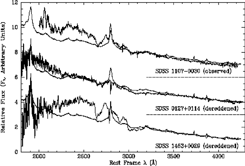
Figure 12: Bottom: the spectrum of SDSS 1453+0029 dereddened by $E(B-V)$=0.5 and plotted atop the composite SDSS quasar after normalizing the two spectra at $>$3350 Å in the rest frame. Middle: the spectrum of SDSS 0127+0114 dereddened by $E(B-V)$=0.36 and similarly plotted atop the composite SDSS quasar. The dotted lines indicate the zero flux levels for this spectrum and the top one. Top: the spectrum of the extreme Fe ii-emitting quasar SDSS J110747.45$-$003044.2 plotted atop the composite SDSS quasar to illustrate how much stronger the Fe ii emission complexes at 2200-2630 Å and 2700-3000 Å are in such objects. What looks like a detached Mg ii BAL trough at 2630-2700 Å in the observed spectrum of SDSS 1453+0029 is actually the gap between Mg ii+Fe ii UV62,63 emission and Fe ii UV1,64 emission shortward of $\sim$2630 Å. Similarly, gaps between Mg ii and Fe ii UV78 emission and Fe ii UV78 and Fe ii Opt6,7 produce apparent troughs at 2900 Å and 3000-3150 Å, respectively.

We estimate SMC reddenings of $E(B-V)$=$0.50\pm 0.05$ for SDSS 1453+0029 and $E(B-V)$=$0.36\pm 0.03$ for SDSS 0127+0114. These dereddened spectra are plotted atop the normalized composite SDSS spectrum in Figure 12, along with the observed spectrum of the extreme Fe ii-emitting quasar SDSS J110747.45$-$003044.2 (Schneider et al. 2002). SDSS 0127+0114 is clearly a normal-to-strong Fe ii emitter, while SDSS 1453+0029 is intrinsically an extreme Fe ii-emitting quasar similar to SDSS J110747.45$-$003044.2 or Q 2226$-$3905 (Graham et al. 1996). What looks like a detached Mg ii BAL trough at 2630-2700 Å in the observed spectrum of SDSS 1453+0029 is actually the gap between Mg ii+Fe ii UV62,63 emission and Fe ii UV1,64 emission shortward of $\sim$2630 Å. Similarly, gaps between Mg ii and Fe ii UV78 emission and Fe ii UV78 and Fe ii Opt6,7 produce apparent troughs at 2900 Å and 3000-3150 Å, respectively. Fe ii emission this strong remains a challenge for quasar models (e.g., Sigut & Pradhan 1998).

5.3.3 Extremely Reddened BAL Quasars

SDSS has discovered several extremely reddened BAL quasars whose emission lines in the observed optical are very weak or absent, somewhat reminiscent of Hawaii 167 (Cowie et al. 1994). For these objects we assume that the onset redshifts of the absorption troughs are the systemic redshifts; where present, the weak C iii] lines are consistent with these redshifts. We discuss the observed spectral slopes of these objects in terms of $\alpha_{\nu}$, where $F_{\nu}\propto\nu^{\alpha_{\nu}}$. For reference, the SDSS quasar composite has $\alpha_{\nu}=-0.44\pm 0.10$, and Gregg et al. (2002) adopted $\alpha_{\nu}\lesssim-1$ as their working definition of a red quasar.

SDSS 0947+6205

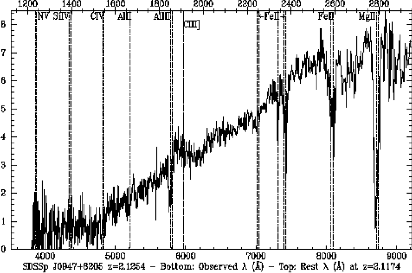
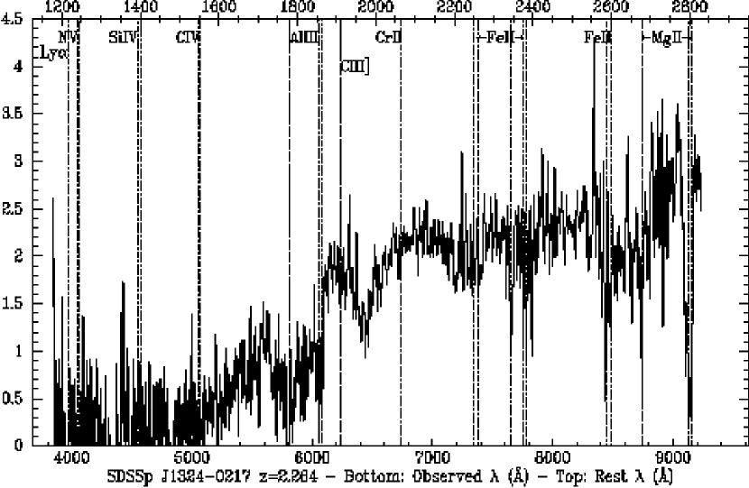
Figure 13: Extremely reddened BAL quasar spectra, smoothed by a 7-pixel boxcar. Observed wavelengths are shown on the bottom axes, and rest frame on the top. Dashed lines show emission, and dotted lines absorption. a) SDSS 0947+6205 at $z=2.1254$. The absorption lines are identified at $z=2.1174$, the redshift of peak absorption. b) SDSS 1324$-$0217 at $z=2.264$. The dot-dashed lines show Al iii and Mg ii in the broad absorption system at $z=2.123$. The absorption at $\sim$6400 Å observed, longward of the C iii] emission, may be due to Fe iii UV48 ($\sim$2070 Å) absorption in this system, and Fe iii UV34 absorption ($\sim$1910 Å) may be present as well, at $\sim$6000 Å observed.

SDSS 0947+6205 (Figure 13a) is at $z=2.1254\pm 0.0006$ from Fe ii and Mg ii absorption. The Mg ii absorption trough spans some 3700$\pm$200 km s^-1, but the BI=0 since C iv region is too noisy to measure and the Mg ii absorption begins at the systemic redshift. The top axis of Figure 13a gives the rest wavelength at the peak absorption redshift of $z=2.1174\pm 0.0007$ (detachment $v=770\pm 90$ km s^-1). Al ii, Al iii, and C iv absorption are also present, detached by 1500$\pm$70 km s^-1 and with a narrower velocity width of 3700$\pm$200 km s^-1. We measure a spectral slope of $\alpha_{\nu}=-4.7\pm 0.1$, and dereddening by $E(B-V)$=0.43$\pm$0.03 brings the spectrum into fair agreement with the SDSS composite. However, there is some suggestion that shortward of Al iii the object’s spectral slope may steepen and the required reddening may increase, or that the reddening curve is different from that assumed, as we discuss below.

SDSS 1324$-$0217

This object (Figure 13b) is at $z=2.264\pm 0.001$ from broad Mg ii, Fe ii, and Al ii absorption; it may also have Al ii and C iv absorption. There is also broad Al iii, Mg ii, and probably Fe iii UV34,48 and weak Fe ii absorption at $z=2.123\pm 0.001$, an outflow velocity of 13230$\pm$130 km s^-1; nonetheless, the object has BI=0. We measure a spectral slope of $\alpha_{\nu}=-2.6\pm 0.1$, but the slope appears to steepen shortward of Al iii. Dereddening the spectrum to match the SDSS composite confirms this steepening, which could be intrinsic or due to an extinction curve different from that of the SMC. We discuss this in detail in §6.3, but here we simply quote the values of $E(B-V)$ needed to bring the object spectrum into agreement with the composite at different wavelengths, using the SMC extinction curve. A reddening of $E(B-V)$=0.2$\pm$0.05 is required at 2000$-$2800 Å, but $E(B-V)$=0.5$\pm$0.05 is required at 1500$-$2000 Å.

SDSS 1456+0114

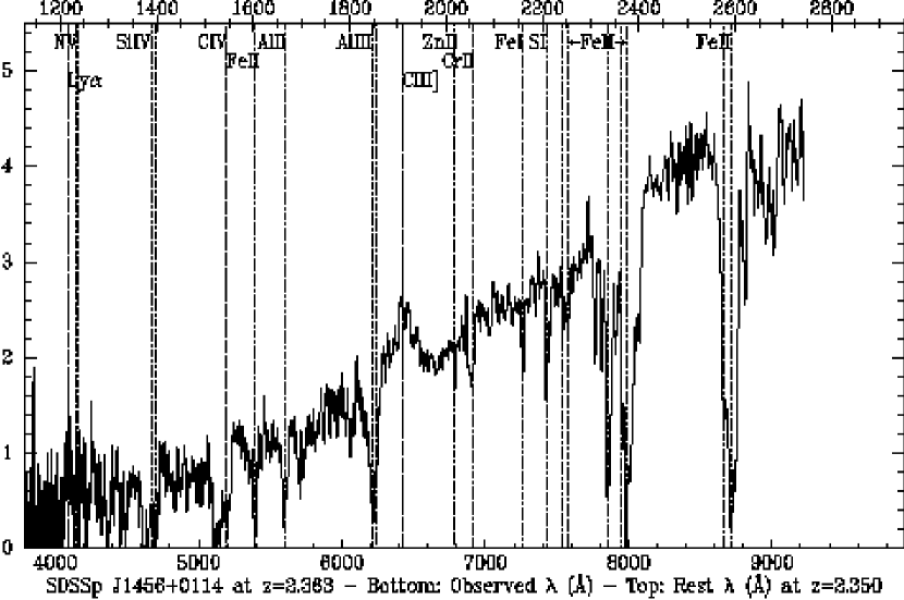
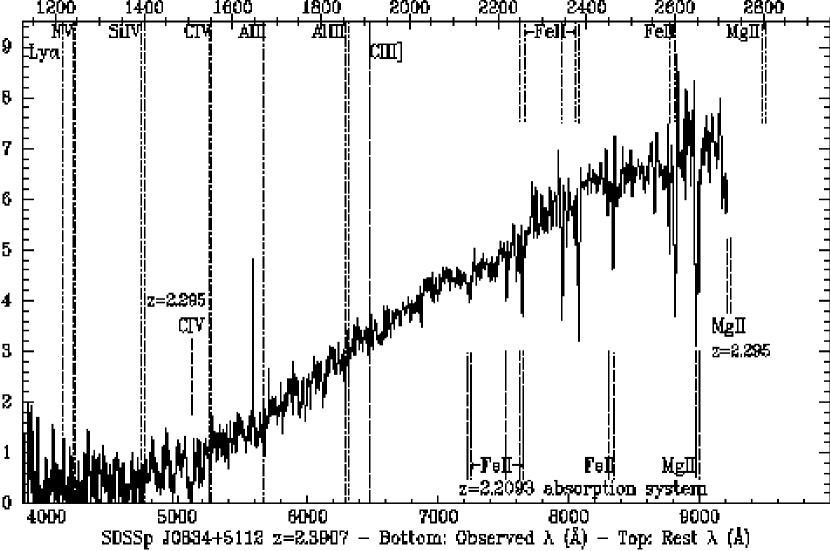
Figure 14: Extremely reddened BAL quasar spectra, smoothed by a 7-pixel boxcar. Observed wavelengths are shown on the bottom axes, and rest frame on the top. Dashed lines show emission, and dotted lines absorption. a) SDSS 1456+0114 at $z=2.363$. The absorption lines are identified at $z=2.350$, the redshift of peak absorption. b) SDSS 0834+5112 at $z=2.3907$. Absorption lines at this redshift are identified above the spectrum, while absorption lines from the $z=2.295$ and $z=2.2093$ systems are identified by dot-dashed lines in the bottom half of the figure.

For this extremely reddened FIRST-detected BAL quasar (Figure 14a) we adopt $z=2.363\pm 0.008$. It shows broad C iii] emission, weak narrow Ly$\alpha$ emission, and broad C iv, Al iii and Fe ii absorption along with narrow Si i, Zn ii, Cr ii, Fe i and S i absorption at the deepest part of the trough, $z=2.350\pm 0.001$ (the top axis of Figure 14a gives rest wavelengths at this redshift). We measure a spectral slope of $\alpha_{\nu}=-4.6\pm 0.1$, and there is no evidence for any deviation from that slope. Dereddening by $E(B-V)$=0.40$\pm$0.05 is required to match the SDSS composite.

SDSS 0834+5112

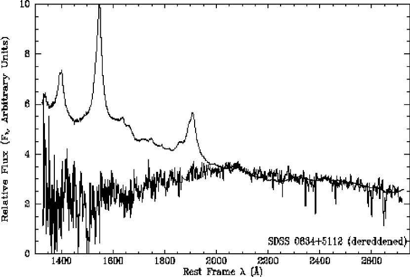
Figure 15: Spectrum of SDSS 0834+5112 smoothed by a 7-pixel boxcar and dereddened by $E(B-V)$=0.3 with the SMC extinction curve to match the SDSS composite quasar from 2000-2800 Å. To reproduce the composite spectrum from 1500-2000 Å as well would require a steeper extinction curve. SDSS 1324$-$0217 and possibly SDSS 0947+6205 also show evidence for a break in their dereddened spectra, but SDSS 0834+5112 is the only one of our extremely reddened objects with sufficient SNR to robustly detect it.

This object (Figure 14b) is a FIRST source at $z=2.3907\pm 0.0002$ from Mg ii, Fe ii, Al iii, and weak C iv absorption. The object has two detached absorption troughs: one at $z=2.295\pm 0.005$ in broad C iv and Mg ii, and one at $z=2.2093\pm 0.0003$ in narrow Mg ii, Fe ii, Al iii, C iv and Si iv. This latter system could be intervening; the SNR is not high enough to tell if its C iv absorption is broad. This object cannot be adequately fit by a single power law. The spectrum steepens from $\alpha_{\nu}=-2.6\pm 0.1$ at 2450$-$2725 Å to $\alpha_{\nu}=-4.4\pm 0.1$ at 2000$-$2450 Å and again to $\alpha_{\nu}=-6.9\pm 0.3$ at 1550$-$2000 Å. Because of this steepening of the continuum, dereddening by $E(B-V)$=0.3$\pm$0.05 is required to match the SDSS composite at 2000$-$2800 Å, but $E(B-V)$=0.65$\pm$0.05 is required at 1500$-$2000 Å (Figure 15).

SDSS 0342+0045

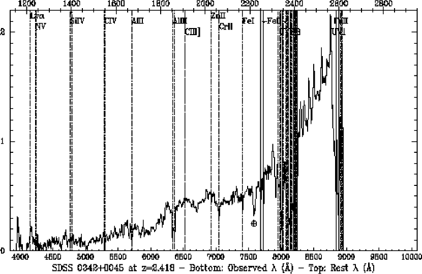
Figure 16: Keck spectrum of SDSS 0342+0045 (smoothed by a 7-pixel boxcar), another extremely reddened BAL quasar, at $z=2.418$. Observed wavelengths are shown on the bottom axes, and rest frame on the top. Dashed lines show emission, and dotted lines absorption. Wavelengths of Fe ii absorption from multiplets UV1, UV2, and UV3 are indicated with lighter dotted lines.

We adopt $z=2.418\pm 0.001$ for this FeLoBAL (Figure 16) from numerous absorption lines. The spectrum shown was obtained at Keck II using LRIS on UT 15 Oct 1999. There is weak C iv absorption and maybe weak Ly$\alpha$+N v emission, but the spectrum is dominated by strong Fe ii absorption (multiplets UV1,2,3 at least). It is obvious from comparison to Figures 13 and 14 that this is a somewhat different sort of extremely reddened BAL quasar. Instead of the spectrum steepening at shorter wavelengths, it flattens out. This is what is expected for a range of reddenings along the sightlines to the emission regions: the heavily reddened sightlines contribute only at longer wavelengths, while less reddened sightlines dominate at shorter wavelengths. We find that dereddening by $E(B-V)$=0.7$\pm$0.1 is required to match the SDSS composite between 2050$-$2550 Å, while only $E(B-V)$=0.42$\pm$0.02 is required between 1250$-$1850 Å.

5.3.4 SDSS 0318$-$0600: A Bright, Reddened FeLoBAL

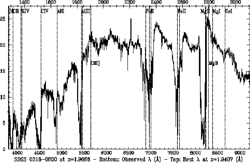
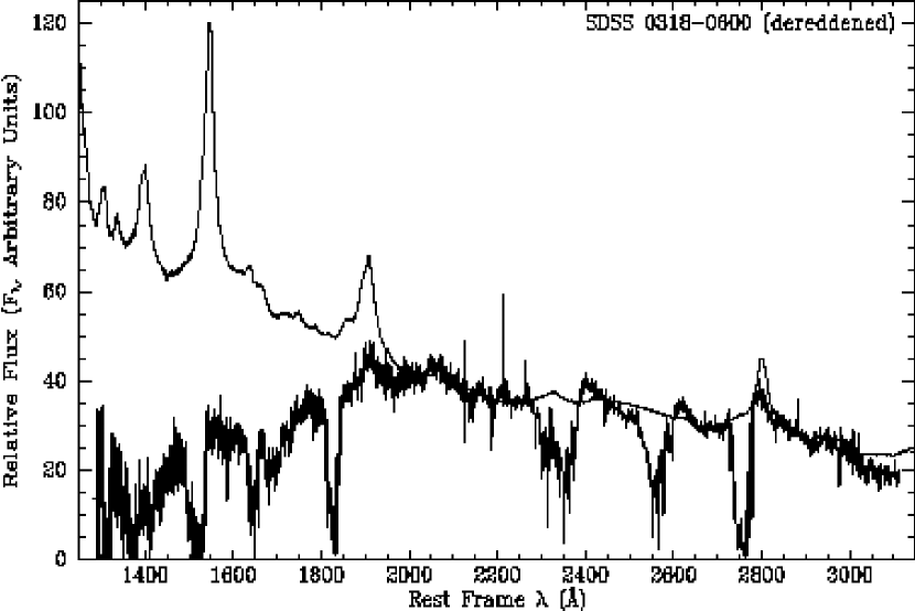
Figure 17: a) SDSS 0318$-$0600 at $z=1.9668$, smoothed by a 3-pixel boxcar. C iii] and Mg ii emission lines at this redshift are indicated by dashed lines and labels beneath the object’s spectrum. Dotted lines indicate absorption at $z=1.9407$ from the highest-redshift absorption system present; the absorption just longward of Al ii is probably due to a combination of Ni ii and Fe ii UV38. Broad Fe ii emission is also visible at 2400 Å and 2600 Å. Note the poorly subtracted telluric H$\alpha$ emission line from auroral activity the night of this observation. b) SDSS 0318$-$0600 dereddened by $E(B-V)$$\sim$0.1 with the SMC extinction curve to match the SDSS composite at rest wavelength $>$2000 Å. To match at $<$2000 Å as well requires an extinction curve steeper even than that of the SMC.

The evidence in several objects in the previous section for a reddening curve steeper than that of the SMC is confirmed in dramatic fashion by this object. SDSS 0318$-$0600 (Figure 17a) has $z=1.9668\pm 0.0015$ from cross-correlation with the SDSS composite quasar of Vanden Berk et al. (2001). It has flux down to at least 1300 Å rest frame and shows absorption from a large number of transitions, few of which appear to reach zero flux. It is similar to FBQS 1044+3656 (de Kool et al. 2001), except that Mg i $\lambda$2852 absorption is only tentatively detected, along with He i $\lambda$2945.

The long wavelength edges of the BAL troughs are at $z=1.9407\pm 0.0006$ (a detachment velocity of 2650$\pm$160 km s^-1), with the strongest absorption at $z=1.9265\pm 0.0006$. The C iv trough extends to an outflow velocity only 3000 km s^-1 higher than the Mg ii trough. The absorption just longward of Fe ii $\lambda$2600 from the highest-redshift system ($z=1.9407$) shows that excited-state Fe ii absorption is present. Multiplets UV1, UV2, and UV3 can be firmly identified, but more may be present. The absorption just longward of Al ii, at $\sim$5000$-$5100 Å observed, is probably due to a combination of Ni ii and Fe ii UV38.

Dereddening the spectrum by $E(B-V)$$\sim$0.1 using the SMC extinction curve brings its slope into agreement with that of the SDSS composite quasar at 2000-3000 Å rest frame, but $E(B-V)$$\sim$0.4 is required to bring the slope at 1250-2000 Å into agreement with the composite (Figure 17b). Note that SDSS 0318$-$0600 is detected by 2MASS, with $J=16.00\pm 0.08$, $H=15.58\pm 0.10$ and $K_{s}=15.02\pm 0.14$. Its near-IR colors are bluer than those of most quasars, indicating that the above $E(B-V)$ may be somewhat underestimated.

The implications of our observations of SDSS 0318$-$0600 and all the other objects presented earlier in this section are discussed in §6.3. We end this section on heavily reddened BAL quasars with a discussion of an object possibly similar to SDSS 0318$-$0600.

5.3.5 SDSS 0338+0056: Reddened Emission or Reddened Absorption?

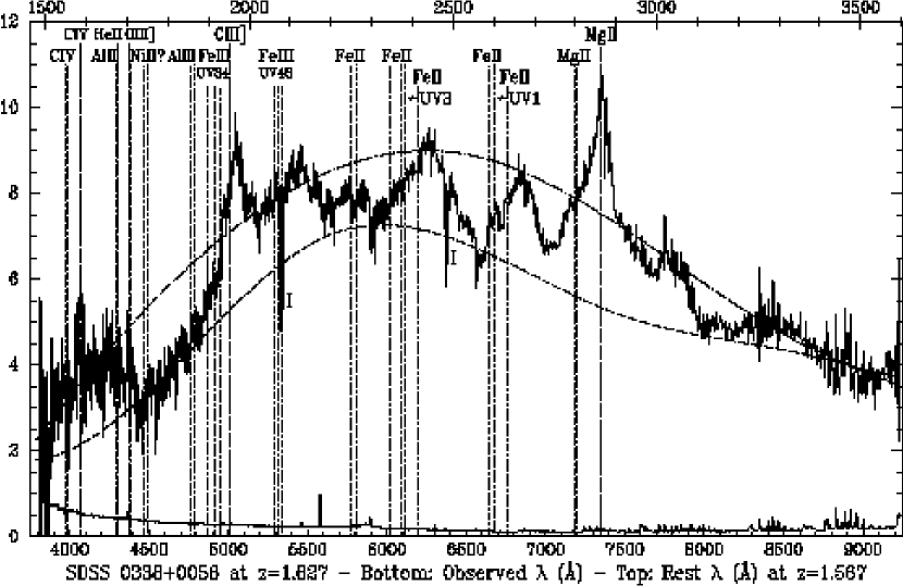
Figure 18: SDSS 0338+0056 at $z=1.627\pm 0.002$. Emission lines at this redshift are indicated with vertical dashed lines. Absorption lines at $z=1.567$, the assumed onset of the BAL troughs, are indicated with vertical dotted lines. Thin vertical dotted lines indicate absorption lines that are not definitely present. For Fe ii UV3 and UV1 multiplets, the wavelength of the longest-wavelength line is plotted and arrows are drawn to indicate the presence of other lines to the blue. There are two intervening Mg ii systems marked ‘I’ beneath the spectrum. The dot-dashed line shows the continuum fit used to calculate the BI and AI. The dashed line shows a possible continuum fit if this object is a reddened strong Fe ii-emitting quasar instead of a BAL quasar.

In SDSS 0338+0056 at $z=1.627\pm 0.002$, the spectrum declines precipitously shortward of C iii] (Figure 18). This decline is confirmed by the object’s $u-g$ color. The spectrum between C iii] and Mg ii seems to be a blend of Fe ii emission and Mg ii and Fe ii absorption, but the object is not yet definitively understood. We outline two possible interpretations here.

The object may be a strong Fe ii-emitting quasar which is reddened with an extinction curve steeper than that of the SMC. In this interpretation, the approximate continuum is given by the dashed line in Figure 18 and the apparent BAL troughs are in fact just gaps between strong Fe ii emission multiplets. The smoothness of the spectrum from 1750$-$1900 Å is hard to explain in this model, since there are Fe ii multiplets in that wavelength range. However, the object does resemble SDSS 0318$-$0600 (§5.3.4) without the BAL troughs, so we consider this interpretation is plausible.

Alternatively, the object may be a reddened BAL quasar with strong Al iii+Fe iii UV34 absorption. In this interpretation, the continuum shortward of Mg ii is given by the dot-dashed line in Figure 18. There is a good match between the putative troughs of Fe iii UV34, Fe ii UV1, Fe ii UV3 and Mg ii. Also, Fe iii UV34 absorption would be stronger than Fe iii UV48 absorption, which is normal. However, Al ii absorption is weak at best and the start of a C iv trough is not clearly detected. If better SNR in the blue confirms the lack of a C iv BAL, then this BAL quasar hypothesis would be ruled out. Even if the BAL hypothesis is correct, the apparently wider trough in Al iii than in Mg ii would require explanation. It could be due to unusually strong Ni ii absorption at the high-velocity end of the apparent Al iii trough, high-velocity Mg ii absorption masked by Fe ii emission, or an overestimated continuum level at $<$1750 Å due to strong He ii+O iii emission. In the latter case, the BAL quasar model continuum should match the reddened strong-Fe ii-emitter model continuum at $<$1750 Å. The resulting very steep drop in the continuum at $<$1900 Å would require either an extinction curve steeper than that of the SMC or a red continuum with the same origin as the red continua of the mystery objects of §5.5, whatever that origin is.

5.4 BAL Quasars with Strong Fe iii Absorption

5.4.1 SDSS 2215$-$0045

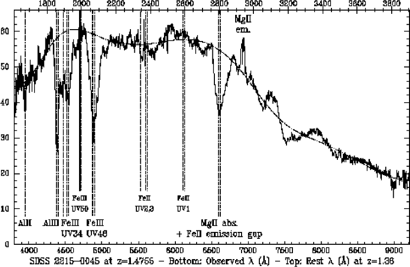
Figure 19: SDSS 2215$-$0045 at $z=1.4755$. The top axis plots rest wavelengths at the peak absorption trough $z=1.36$, rather than this emission-line $z$, to demonstrate the absence of Fe ii absorption at 2200$-$2600 Å. The thick dotted lines show detected absorption troughs, while the thin dotted lines show the expected positions of troughs that are not detected. The dot-dashed line shows the continuum fit used to normalize the spectrum for calculation of the BI and AI, and for plotting the following Figure.

SDSS 2215$-$0045 (Figure 19) is a reddened LoBAL with detached Mg ii $\lambda\lambda$2796,2803, Al iii $\lambda\lambda$1854,1862, Al ii $\lambda$1670, and Fe iii absorption. Our redshift $z=1.4755\pm 0.0002$ is set by narrow associated Mg ii absorption seen atop a weak broad Mg ii line. SDSS 2215$-$0045 is detected by 2MASS, with $J=15.68\pm 0.08$, $H=14.89\pm 0.07$ and $K_{s}=14.71\pm 0.10$. Its near-IR colors are bluer than most quasars. This is consistent with the spectrum longward of 3000 Å, which is as blue as the SDSS composite. The spectrum shortward of 3000 Å, however, appears to be reddened by $E(B-V)$ $\simeq 0.15\pm 0.05$ compared to the SDSS composite. This will be a lower limit to the reddening if SDSS 2215$-$0045 is indeed bluer than the average quasar.

By comparison to SDSS 1723+5553 (Figure 5, bottom left corner), we initially identified the strong trough at $\lambda_{obs}$$\sim$4900 Å as Cr ii $\lambda$$\lambda$$\lambda$2056,2062,2066. However, the implied relative abundance of Cr is implausible, and the expected corresponding Zn ii is missing. This absorption is in fact due to Fe iii UV48 $\lambda$$\lambda$$\lambda$2062.21,2068.90,2079.65 (EP=5.08 eV). There is also Fe iii UV34 $\lambda$$\lambda$$\lambda$1895.46,1914.06,1926.30 (EP=3.73 eV) absorption longward of Al iii, at $\lambda_{obs}$$\sim$4500 Å. However, Fe ii absorption is weak at best. No Fe ii absorption troughs are detectable to a limit of 10% of the strength of the Fe iii troughs. In addition, Mg ii absorption is probably much weaker than it appears. There are gaps between Fe ii emission complexes at $\sim$2670 Å (rest-frame), the same wavelength as the detached Mg ii absorption, and at $\sim$3100 Å (e.g., Figure 12). Given the strength of the Fe ii emission around the 3100 Å gap, most of what appears to be detached Mg ii absorption in SDSS 2215$-$0045 could be due to the 2670 Å gap. However, the presence of other absorption troughs at this redshift argues that some Mg ii absorption is present. Both Fe ii emission modeling and spectropolarimetry would be useful in untangling this object’s absorption troughs from its Fe ii emission.

In Figure 20 we plot the normalized spectrum of SDSS 2215$-$0045 around the troughs of Mg ii, Fe iii UV48, Fe iii UV34, Al iii, and Al ii. All troughs were normalized using the continuum fit shown as the dot-dashed line in Figure 19, though as discussed above, the Mg ii trough is confused with complex Fe ii emission. The strength of the Mg ii trough could well be less than shown, and its velocity structure is also untrustworthy. The troughs are plotted in terms of blueshifted velocity from systemic; for multiplets, the velocity is for the longest wavelength line. The dot-dashed vertical lines show the wavelengths of every line of each multiplet at 14300 km s^-1, the central velocity of the Al ii absorption.

Within the uncertainties, the troughs appear to have the same velocities for their peak absorption, and all troughs except for Al ii are consistent with having the same starting and ending velocities (6000 and 18000 km s^-1, respectively). The absorption troughs are thus unusual for a LoBAL in that they are strongest near the high-velocity end rather than near the low-velocity end. At the velocity of peak absorption the normalized depths of the Fe iii UV48 and Al iii lines are the same, within the uncertainties. This suggests that they share the same partial covering factor. The Al ii and Fe iii UV34 troughs are not as deep; this is probably because they are not saturated, rather than the depth being a reflection of covering fraction, since Fe iii UV34 and Fe iii UV48 absorption should have the same covering factor.

Finally, the relative strengths of UV48 and UV34 absorption are reversed in this object compared to other BAL quasars with Fe iii (e.g., SDSS 1723+5553, §5.1.1). We discuss the implications of this in §6.2.

5.4.2 Other BAL Quasars With Possible Strong Fe iii Absorption

We have found several other candidate strong Fe iii absorbing BAL quasars besides SDSS 2215$-$0045, though none with Fe iii absorption as strong relative to Mg ii as in that object. The criteria we use for selecting such candidates is the presence of a trough at $\sim$2070 Å which is stronger than Fe ii UV1,2,3 troughs near 2400 Å and 2600 Å. When such Fe ii troughs are present with strength comparable to or greater than the 2070 Å trough, Cr ii is a more likely identification for the latter than Fe iii.

We note in passing that PC 0227+0057 (Schneider, Schmidt, & Gunn 1999) has been identified as a similar object at $z\simeq 1.52$. It has weak Fe ii absorption, but its 2070 Å trough probably includes a contribution from Fe iii. The trough is too strong relative to the Fe ii troughs to be due solely to Cr ii.

SDSS 1214$-$0001

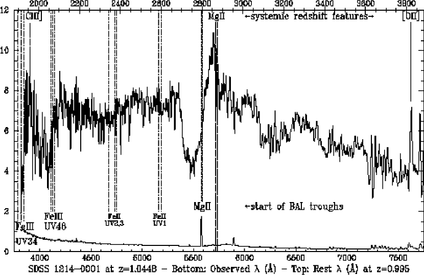
Figure 21: Partial spectrum and error array of SDSS 1214$-$0001 (data at $>$7750 Å are not plotted due to very poor night sky line subtraction). [O ii] emission and Mg ii absorption define the systemic redshift $z=1.0448$. There are broad Mg ii peaks just shortward of this $z$, and there is possible weak C iii] at this $z$ within the uncertainties (dashed lines show features at the systemic $z$). The top axis gives rest wavelengths at the redshift of the start of the BAL troughs, $z=0.995$. Given the absence of strong Fe ii absorption at this redshift (thin dotted lines), and the good match of Fe iii UV34 and Fe iii UV48 troughs to the well-defined Mg ii BAL trough (thick dotted lines), this object is likely similar to SDSS 2215$-$0045.

SDSS 1214$-$0001 (Figure 21) is at $z=1.0448\pm 0.0004$ from associated Mg ii absorption and [O ii] emission (the latter is real, despite being near a night sky line). The peak of the broad Mg ii emission is shortward of this redshift. There is a detached Mg ii trough, but no matching Fe ii troughs. Thus the 2070 Å trough is likely to be Fe iii UV48. This claim is bolstered by the apparent start of a Fe iii UV34 trough at the blue edge of the spectrum, at a redshift which matches the start of both the Fe iii UV48 and Mg ii troughs. Higher SNR data extended further to the blue are needed to study this object further.

SDSS 0149$-$0114

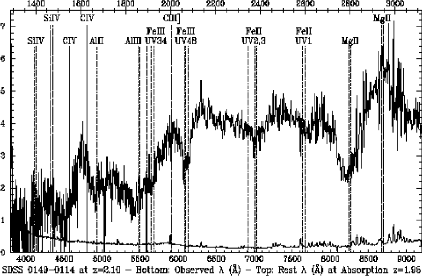
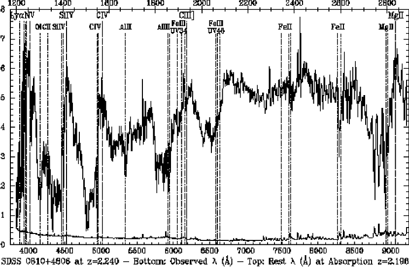
Figure 22: Other SDSS BAL quasars with possible Fe iii UV48 absorption: a) SDSS 0149$-$0114 at $z=2.10\pm 0.01$. b) SDSS 0810+4806 at $z=2.240\pm 0.005$. The error array for each object is plotted along the bottom of each graph.

SDSS 0149$-$0114 at $z=2.10\pm 0.01$ (Figure 22a) has low SNR but does appear to have a narrow Fe iii UV48 trough as well as a broader Mg ii trough and weak Fe ii UV1,2,3 absorption. Higher SNR data are needed to confirm the strong Fe iii UV48 line and to measure the strength of Fe iii UV34.

SDSS 0810+4806

SDSS 0810+4806 at $z=2.240\pm 0.005$ (Figure 22b) may have weak Fe ii UV1,2,3 absorption, but the 2070 Å trough is much stronger than any such absorption, meaning that it is almost certainly Fe iii instead of Cr ii. However, higher SNR data are needed to say anything beyond that.

5.5 The Mysterious Objects SDSS 0105$-$0033 and SDSS 2204+0031

The SDSS has discovered two objects to date with strange but very similar continuum shapes that include dropoffs shortward of Mg ii. Both are FIRST sources with fluxes of a few mJy.

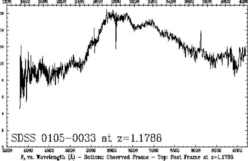
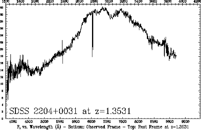
Figure 23: a) SDSS 0105$-$0033 at $z=1.1788$ from Mg ii absorption and [O ii] emission. b) SDSS 2204+0031 at $z=1.3531$ from cross-correlation with the spectrum of SDSS 0105$-$0033. Rest wavelengths are shown at the top and observed wavelengths at the bottom of each plot; both plots have the same rest frame wavelength limits. Both spectra have been smoothed by seven pixels everywhere except at the wavelengths of the associated Mg ii absorption, in order to reduce the noise while illustrating the depth of the Mg ii absorption at the original resolution of $R\sim 1950$.

SDSS 0105$-$0033 has [O ii] $\lambda\lambda$3727,3729 emission at $z=1.1787\pm 0.0007$ (Figure 23a). No other narrow emission lines are present between 1800 AA and 3900 Å (rest-frame), but there may be broad emission features near 4000 Å and 4200 Å, possibly due to Fe ii. There is also unresolved associated Mg ii absorption at $z=1.1788\pm 0.0001$. Given that the [O ii] redshift agrees with this within its errors, we adopt the more accurate Mg ii redshift as systemic. SDSS 0105$-$0033 is detected by 2MASS, with $J=16.31\pm 0.10$, $H=15.81\pm 0.15$ and $K_{s}=14.89\pm 0.13$. Its near-IR colors are typical for quasars.

SDSS 2204+0031 does not show any narrow emission, but it has associated Mg ii absorption at $z=1.3354\pm 0.0001$ (Figure 23b). However, comparison of its spectrum with that of SDSS 0105$-$0033 shows that the various continuum features do not match up if this Mg ii redshift is assumed to be the systemic redshift. Cross-correlation of the two spectra yields a redshift $z=1.3531\pm 0.0009$ for SDSS 2204+0031. The SNR of the cross-correlation peak is $R=2.21$, which is low. However, given the similarity of the continuum features in the two objects, we adopt the cross-correlation redshift for SDSS 2204+0031. This places the Mg ii absorption 2260$\pm$120 km s^-1 shortward of systemic.

Longward of about 3200 Å rest frame, the continuum in both objects is blue and mostly featureless. As seen in Figure 23, moving shortward in the rest frame, both observed (unreddened) spectra show a peak near 3200 Å, a local mininum near 3000 Å, a relatively flat (in $F_{\lambda}$) region with associated Mg ii absorption, a slight drop near 2600-2625 Å, another drop near 2500 Å (stronger in SDSS 0105$-$0033), and finally a continuum which decreases slowly to shorter wavelengths down to at least 1750 Å. The dropoffs shortward of the Mg ii absorption appear too steep to be due to reddening and are not due to obvious BAL troughs.

The only objects with similar spectra that we are aware of are FBQS 1503+2330 ($z=0.492$) and FBQS 1055+3124 ($z=0.404$) both of which have narrow Mg ii absorption and strong broad Fe ii and Balmer line emission at the same redshift (White et al. 2000). FBQS 1503+2330 has no obvious Mg ii emission, while FBQS 1055+3124 has a spectrum near Mg ii closely resembling that of SDSS 0105$-$0033. Just like our two SDSS objects, these objects have dropoffs shortward of Mg ii which are too abrupt to be caused by reddening and are not obviously due to BAL troughs. Since these features are at the blue ends of the spectra, however, they could be due to detached Mg ii BAL troughs or to flux calibration errors (cf. the difference between the spectra of FBQS 1044+3656 in White et al. 2000 and de Kool et al. 2001).

We consider possible explanations for the spectra of these objects in §6.1.

6 Discussion

Having presented five categories of unusual BAL quasars discovered to date in the SDSS, we now discuss their implications for models of BAL outflows and quasars in general. We do so in a somewhat unorthodox reverse order so that our lengthy discussion of quasars with longward-of-systemic absorption comes last.

6.1 Trying to Explain the Mysterious Objects SDSS 0105$-$0033 and SDSS 2204+0031

6.1.1 Reddening

SDSS 0105$-$0033 and SDSS 2204+0031 (§5.5) are not simply reddened normal quasars, since they lack obvious emission lines. However, reddened BAL quasars can have weak emission lines (§5.3.3), and these high-redshift radio sources must be AGN since they are more luminous than any galaxy. Since reddening seems to be present, we attempt to account for it and to see if reddening of unusual AGN can explain the spectra. To estimate the reddening in these objects, we followed the procedure outlined in §5.3.1, except that we interpolated over all strong emission lines in the composite SDSS quasar before comparing to it.

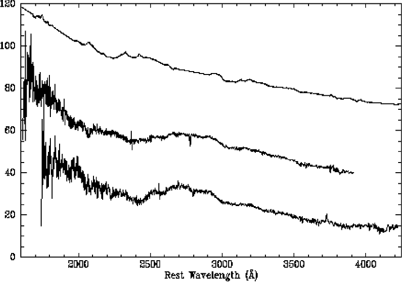
Figure 24: From top to bottom: the SDSS composite quasar, with emission lines interpolated over; the spectrum of SDSS 2204+0031, dereddened by $E(B-V)$=0.32; and the spectrum of SDSS 0105$-$0033, dereddened by $E(B-V)$=0.25 (using the SMC extinction curve). The spectra have been scaled to a common mean and offset vertically in equal steps of 30 flux units. The object spectra have here been smoothed by seven pixels everywhere, including at the wavelengths of the associated Mg ii absorption systems.

Even before dereddening, both objects are roughly as blue as the composite when all three spectra are measured at rest wavelengths 3000$-$3900 Å. Therefore, if reddening is present, these objects must be intrinsically bluer than the average quasar. By considering the entire 1800-3900 Å region, we estimate minimum reddenings of $E(B-V)$ $=0.25\pm 0.05$ for SDSS 0105$-$0033 and $E(B-V)$ $=0.32\pm 0.03$ for SDSS 2204+0031 using the SMC extinction curve at the quasar redshift. The dereddened spectra are compared to the composite spectrum in Figure 24.

Some quasars have very weak Mg ii emission but normal Fe ii emission, and some have very strong Fe ii emission (e.g., §5.3.2). Are the strange continua of SDSS 0105$-$0033 and SDSS 2204+0031 consistent with reddened versions of such quasars? Some Fe ii emission may be present in these two objects — the peak near 3200 Å seen in many quasar spectra is usually ascribed to Fe ii Opt6,7 and the local minimum near 3000 Å to a gap between Fe ii multiplets UV78 and Opt6,7+[O iii] (Vanden Berk et al. 2001) — but their spectra shortward of Mg ii do not show emission at the wavelengths of Fe ii multiplets seen in normal and strong Fe ii emitters (compare Figure 24 to Figure 11b).

Thus, while reddening may be present in these objects, it cannot fully explain their unusual spectra.

6.1.2 BAL Troughs with Spatially Distinct Partial Covering?

The two FBQS objects similar to these two SDSS objects (§5.5) have strong Fe ii emission. Since strong Fe ii emission and the presence of BAL troughs are correlated (Boroson & Meyers 1992), this suggests that all four objects are indeed BAL quasars. If so, shorter wavelength spectra of the two FBQS objects should reveal detached but otherwise normal BAL troughs. For the two SDSS objects a more unusual type of BAL trough is required, as follows, but even that does not provide a very satisfactory explanation.

We can achieve barely plausible fits for the two SDSS objects as BAL quasars with Mg ii, Fe ii $\lambda$2750, and Fe ii $\lambda$2600 troughs $\gtrsim$20,000 km s^-1 wide and detached by $\sim$12300 km s^-1. However, Fe ii$\lambda$2400 seems weaker than expected. Moreover, most BAL quasars have troughs which are saturated in most transitions even if there is only partially covering of the continuum source (Arav et al. 2001b). Thus the absorption does not appear twice as strong when two troughs overlap (i.e., when two species have different outflow velocities such that they produce absorption at the same observed wavelength). In contrast, explaining these objects as BAL quasars requires absorption that increases in strength when troughs overlap. Unsaturated absorption would do this, but the putative Fe ii $\lambda$2600 absorption here is much too strong relative to Mg ii for the troughs to be unsaturated.

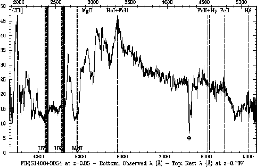
Figure 25: Spatially distinct velocity-dependent partial covering in FBQS 1408+3054 (White et al. 2000). Emission lines are listed along the top, and absorption lines along the bottom. Where high velocity Fe ii UV1 absorption overlaps with low velocity Fe ii UV2 absorption, the absorption increases in strength. For saturated BAL troughs arising from the same terms of the same ion, that cannot happen unless the flow partially covers different source regions as a function of velocity.

The only other way to produce absorption which increases in strength when troughs overlap is to have partial covering of different regions of the continuum source as a function of velocity. Partial covering of the same region of the source with velocity is what is seen or assumed in most BAL quasars (e.g., §3.3 of de Kool et al. 2001). The only object known to definitely exhibit spatially distinct velocity-dependent partial covering is FBQS 1408+3054 (Figure 25; spectrum from White et al. 2000). The Fe ii UV1 trough in this object has smaller partial covering than the Mg ii trough. However, where the high velocity end of the Fe ii UV1 trough overlaps with the low velocity end of the Fe ii UV2,3 trough, at 4300 Å observed, the absorption increases in depth. (Contrast this with the top panel of Figure 5, where all Fe ii troughs have the same apparent partial covering even when they overlap.) Different partial covering of the same source region cannot explain this, since Fe ii UV1, UV2, and UV3 absorption arise from the same term of Fe ii. Nor can the gas be optically thin since Fe ii absorption would not be nearly as strong relative to Mg ii in that case. The Fe ii gas must partially cover different regions of the continuum source as a function of velocity.

Spatially distinct velocity-dependent partial covering may not be all that rare, just difficult to recognize. Unless the spatial regions covered change rapidly with velocity, such partial covering would be obvious only when two troughs overlap at substantially different velocities. Troughs that wide are uncommon and not very well studied. Nonetheless, given that even with this type of partial covering the fits for these objects as BAL quasars are barely plausible, we consider other possible explanations for these objects.

6.1.3 BAL Troughs Plus Double-Shouldered Mg ii Emission?

The region from 2500–3200 Å in these objects could be a region of continuum emission plus extremely broad ‘double-peaked’ or ‘double-shouldered’ Mg ii emission produced by an accretion disk (e.g., Arp 102B, cf. Figure 1 of Halpern et al. 1996). If so, the full width at zero intensity (FWZI) in both objects would be about 40,000 km s^-1, twice the FWZI of the double-shouldered lines in Arp 102B. Halpern et al. (1996) model Arp 102B as an accretion disk inclined by 32° to the line of sight. The same disk viewed edge-on would have a FWZI 1.9 times larger, so a FWZI of 40,000 km s^-1 is possible. The observed reddening is probably consistent with an edge-on line of sight.

However, as seen in Figure 24, to explain the dereddened continuum shape shortward of Mg ii, the double-shouldered emission line hypothesis may require shallow, smooth absorption troughs from $\sim$2050-2500 Å rest frame in SDSS 0105$-$0033 and $\sim$1900-2500 Å rest frame in SDSS 2204+0031. There are Fe ii transitions in this wavelength range, but they should be accompanied by Mg ii absorption. We therefore must identify the start of the trough at 2500 Å with Mg ii absorption detached by 35,000 km s^-1. The absorption must also reach an outflow velocity of $\geq$53,000 km s^-1 so that the Mg ii and Fe ii UV1,2,3 troughs all overlap to produce a single smooth trough. Both the detachment and peak outflow velocities are very large for low-ionization BAL troughs, but not unprecedented (§5.2). Alternatively, the difference between the dereddened continuum shapes and the composite may be due to the absence of Fe ii emission in these two objects. Similarly, adding a small 2200 Å bump to the SMC extinction curve might eliminate the need for these broad, shallow absorption troughs, and the drop near 2500 Å could be explained as a moderately broad detached Mg ii trough (cf. SDSS 2215$-$0045; §5.4.1) with little or no accompanying Fe ii absorption.

6.1.4 Other Possible Explanations

Our two SDSS objects are FIRST sources, but radio-quiet. Thus the peaks in the spectra near Mg ii in these objects cannot be due to the turnover of a red synchrotron component (e.g., Francis, Whiting, & Webster 2000). These objects are not supernovae, as supernovae have redder colors at these rest wavelengths. They are not galaxies at the redshifts of the Mg ii absorption which are gravitationally lensing higher-redshift quasars, since there are no signs of emission lines or Ly$\alpha$ forest absorption from such quasars. Neither object shows any sign in its images or spectrum of being a superimposition of two quasars or a quasar and a star or galaxy. One very speculative possible explanation is emission from an accretion disk with a gap in the regions hot enough to produce significant emission at $\lambda_{rest}<2800$ Å. Such a gap is unlikely to be long-lived, so future observations of these objects could test this hypothesis.

One last possibility is a reddened version of PG 1407+265 (McDowell et al. 1995), which has very weak emission lines shortward of Mg ii, and emission lines increasingly blueshifted with ionization potential, up to a maximum of 10,000 km s^-1 in C iv relative to H$\alpha$. Reddened quasars with weak Mg ii and weak, blueshifted C iii] might explain these objects, though their detailed continuum structure would still be puzzling.

6.1.5 Summary

None of the three viable explanations for these objects — BAL quasars with spatially distinct partial covering, double-shouldered emission line objects, or reddened PG 1407+265 analogs — are particularly satisfactory. The spatially distinct partial covering hypothesis predicts these objects should have other properties similar to BAL quasars: e.g., weak X-ray emission, strong Fe ii and weak [O iii] emission, and high polarization, especially in the BAL troughs. The double-shouldered hypothesis can be tested by studying the line profiles of H$\beta$ or H$\alpha$ in the near-IR or of C iv in the atmospheric UV; our spectra are unfortunately too noisy to determine if there is double-shouldered H$\delta$ emission in either object. The reddened PG 1407+265 hypothesis can be tested with high-SNR spectra of C iii] and C iv, as well as H$\beta$ and H$\alpha$.

Finally, note that it is possible that both the [O ii] emission and Mg ii absorption in SDSS 0105$-$0033 are from an intervening galaxy. If this is the case then the redshifts of both objects are unknown, since our redshift for SDSS 0105$-$0033 comes from the [O ii] emission in its spectrum and our adopted redshift for SDSS 2204+0031 comes from cross-correlation with SDSS 0105$-$0033. The only remaining constraint for both objects is that $z\lesssim 2.15$ since we do not see Ly$\alpha$ or the Ly$\alpha$ forest.

6.2 Implications of BAL Quasars with Strong Fe iii Absorption

SDSS 2215$-$0045 (§5.4.1) has a nearly unique spectrum, in which Fe iii absorption is much stronger than Fe ii absorption. There are several other possibly similar objects with lower SNR (§5.4.2), but until better data on them are available we discuss only SDSS 2215$-$0045 in detail. A full photoionization calculation of the conditions in the BAL gas in this object is beyond the scope of the present work, so we merely speculate on what conditions might be needed to produce such a strange spectrum.

In SDSS 2215$-$0045, Fe iii absorption is present from terms with different excitation potentials (EP), and absorption in Fe iii UV48 (EP 5.08 eV) is as strong or stronger than in Fe iii UV34 (EP 3.73 eV) or in Fe iii UV50 (EP 7.86 eV). Using line strengths from Nahar & Pradhan (1996), it is easy to show that this can never happen in conditions of local thermodynamic equilibrium (LTE). Nor can it happen if the particle densities are too low for LTE to apply, since then the population of the lower term of Fe iii UV48 would be reduced even further. The lower term of the Fe iii UV48 multiplet must be overpopulated in SDSS 2215$-$0045. This is a rare occurrence; in most BAL quasars where Fe iii is detected, absorption from Fe iii UV34 is stronger than from Fe iii UV48. For example, in SDSS 1723+5553 (Figure 3, top panel), UV34 at $\sim$1910 Å is strong but UV48 at $\sim$2070 Å must be much weaker since the 2070 Å feature can be explained entirely by Cr ii. SDSS J132139.86$-$004152.0 (Menou et al. 2001) also shows Fe iii UV34 but not UV48.

According to Zhang (1996), there are no resonances in the collision strengths to the lower terms of these multiplets strong enough to explain why the lower term of the UV48 multiplet ($a^{5}S$) is overpopulated relative to that of the UV34 multiplet ($a^{7}S$) and the UV50 multiplet ($a^{5}G$). Thus we conclude that in this object the population of the lower term of the Fe iii UV48 multiplet is governed by a fluorescence resonance due to absorption of an emission line (or possibly by recombination from Fe iv to excited Fe iii). In either case the lower term of UV48 could be populated directly or indirectly. The latter would be via population of an even more excited term followed by a cascade of emission down to the lower term of UV48, though the lack of UV50 absorption means that any cascade does not involve the lower term of that multiplet. Johansson et al. (2000) show that there is a direct resonance with Ly$\alpha$ from the ground term of Fe iii ($a^{5}D$) to the lower term of Fe iii UV34, but that the transitions from the ground term to the lower term of Fe iii UV48 are weak and forbidden. Thus, if a fluorescence resonance is at work, it is probably a indirect one.

The other unusual aspect of the absorption in this quasar is that Fe iii is much stronger than Fe ii, and probably stronger than Mg ii as well. In most BAL regions, where the ionization parameter is large and the densities may not be high enough for LTE to apply, the ratio Fe iii/Fe ii (as well as Mg iii/Mg ii and Al iii/Al ii) will be determined by photoionization equilibrium rather than by the Saha equation. Thus, without detailed modeling, we can only conclude that the gas producing the observed BAL trough in SDSS 2215$-$0045 must be of moderately high ionization, and with a high enough column density to produce appreciable Fe iii absorption. Given this requirement, and the observed strength of its absorption relative to Fe ii, Fe iii is probably the dominant Fe ion. Note that such a highly ionized BAL region should also have a high temperature; if so, the observed reddening must be produced by dust outside the BAL region.

In the Murray & Chiang (1998) and Elvis (2000) disk wind models for BAL quasars, detached troughs such as those in SDSS 2215$-$0045 are seen along lines of sight which skim the upper surface of the outflow, which is more highly ionized than the rest of the flow. The unique highly ionized HiBAL SBS 1542+541 (Telfer et al. 1998) might be seen along such a line of sight. Similarly, the uniqueness of SDSS 2215$-$0045 might stem from its being unusual in three ways: a FeLoBAL quasar seen along a line of sight through the highly ionized upper surface of a disk wind, and with a column density through the wind high enough so that considerable Fe iii absorption is seen. Alternatively, since at least some quasars experience a phase of high-covering-factor LoBAL absorption in their youth (Canalizo & Stockton 2001), SDSS 2215$-$0045 might be a ‘teenage’ quasar captured in the act of ionizing away its youthful BAL cocoon. Lastly, the unusual absorption might be due to an unusual spectral energy distribution for this quasar. Photoionization modeling of the BAL gas in SDSS 2215$-$0045 and other strong-Fe iii-absorption BAL quasars, especially ones with narrower troughs, is needed to understand what is special about such objects, and why they are so rare.

6.3 Implications of Heavily Reddened BAL Quasars

We are aware of only three BAL quasars with extinctions greater than those seen in our extremely reddened BAL quasars (§5.3.3). Hawaii 167 has $E(B-V)$$\simeq$0.54–0.7 (Egami et al. 1996) and FIRST 0738+2750 has $E(B-V)$$\simeq$0.7 (Gregg et al. 2002). FIRST 1556+3517 has $E(B-V)$$\simeq$0.6 along the direct line of sight to its central engine, but its observed UV flux is dominated by a scattered component with $E(B-V)$$\simeq$0.1 (Najita, Dey, & Brotherton 2000). Its UV spectrum therefore does not resemble the extremely reddened BAL quasars of §5.3.3; in fact, it is very similar to the overlapping-trough BAL quasars of §5.2.

The detection of numerous heavily reddened quasars in the SDSS lends weight to the growing consensus that a population of red quasars does exist (e.g., Gregg et al. 2002). Quasars do not have to have BAL troughs to be reddened (Richards et al. 2001), but BAL quasars are more often reddened than normal QSOs are (Richards 2001), and there is evidence for dust in the absorbing region of at least one BAL quasar (de Kool et al. 2001). In this section we note a few constraints our reddened BAL quasars (§5.3) place on reddening of quasars by dust.

Dust reddening does not affect equivalent widths, yet many of these objects lack broad emission lines. This may indicate that the broad line region is more heavily reddened than the continuum, which could happen if there is a range of extinctions among the sightlines to the emission regions (Hines & Wills 1995). Alternatively, the majority of the observed flux could be scattered continuum light, a hypothesis which can easily be tested via polarization measurements.

The five extremely reddened BAL quasars we have presented (§5.3.3) all have $2<z<2.5$. Similar objects at $z>2.5$ will usually be too faint for the SDSS to detect or target, but it should be able to find lower-redshift analogs. However, to date we have found no reddened $z<2$ BAL quasars which have emission lines as weak as these objects. Simulating such objects’ colors would help determine if this absence is real or due to their being overlooked by the quasar target selection algorithm.

6.3.1 Extinction Curves in Reddened BAL Quasars

We have seen evidence in several reddened BAL quasars for spectral breaks which might require an extinction curve steeper than that of the SMC. The spectra of hot stars on the spectroscopic plates on which these objects were discovered are unremarkable, so the spectral breaks are not reduction artifacts. We now examine alternative explanations for the spectral breaks as well as possible origins for such extinction curves.

We have not considered the contaminating effects of host galaxy emission, but it could be important only for objects which are very low luminosity. SDSS 0342+0045 is the lowest luminosity object, but the presence of Fe ii absorption indicates it is a BAL quasar. The troughs in it and the other objects are also very deep. This limits the contribution of host galaxy light to typically $\lesssim$20%, even assuming that the troughs are resolved and host galaxy light is entirely responsible for the remaining emission in the troughs.

The apparently different reddenings shortward and longward of 2000 Å in the quasar rest frame are not more easily explained by extinction in a galaxy between us and the quasar instead of by extinction at the quasar redshift. In the ultraviolet through the optical, plausible extinction curves have greater extinctions at shorter wavelengths (except near the 2200 Å bump, for which there is no evidence in the spectra), and the slope of the extinction curve is also greater at shorter wavelengths. Thus the intervening reddening needed to match the composite spectrum at $>$2000 Å would be larger than the intrinsic reddening needed, and even then, the discrepancy at $<$2000 Å would be worse.

BAL quasars may be preferentially viewed edge-on (e.g., Glenn, Schmidt, & Foltz 1994). Limb darkening and relativistic effects should make edge-on accretion disk spectra look different (Czerny & Elvis 1987; Laor & Netzer 1989; Sun & Malkan 1989; Hubeny et al. 2000). However, in all these models, at $\lambda$$\gtrsim$912 Å the dominant effect is limb darkening with a smooth wavelength dependence which does not change the spectra appreciably. Only for one choice of parameters considered by Czerny & Elvis (1987, model 1.5 in their Figure 4) does a change in viewing angle produce a break in the spectrum similar to those observed here. Thus viewing angle effects are unlikely to be the explanation for our spectra.

Turnshek et al. (1994) show that PG 0043+039 appears to have a continuum break at 2400 Å (their Figure 4), but is actually a reddened extreme Fe ii emitter (their Figure 5). Among our objects, however, only SDSS 1453+0029 shows the extreme Fe ii emission required to mimic such a continuum break.

The objects might be intrinsically much bluer than the typical quasar and even more heavily reddened than we estimate, as small differences in the apparent slopes in different spectral regions are exaggerated by very large reddenings. However, the distribution of spectral slopes of unreddened quasars limits the reddening which can reasonably be inferred. For example, if SDSS 0318$-$0600 is reddened by $E(B-V)$$\sim$0.5, it would have an intrinsic $\alpha_{\nu}=1.75$, bluer than essentially all known quasars.

Most of these objects do not match the composites exactly even when dereddened. This is probably just because quasar continuum and emission line properties vary from object to object. However, if strong luminosity or redshift dependencies in quasar spectra exist (e.g., Green, Forster, & Kuraszkiewicz 2001b) then the SDSS composite quasar spectrum might be an incorrect representation of quasars at $z\sim 2$ because the objects that contribute to the composite spectrum at $<$2000 Å are of higher average redshift and luminosity than those that contribute at 2000-3000 Å. Any such dependencies would have to be improbably strong to bias the SDSS composite significantly, as the sample of quasars used to construct the template has a mean $M_{r^{*}}\simeq-24$ at $z=1$ and $M_{r^{*}}\simeq-25$ at $z=2.3$, with only a small number of objects contributing at $z>2.3$.

It is also conceivable that the apparent spectral break in the dereddened spectra of these objects is an intrinsic property, rather than an artifact of dereddening with an inappropriate extinction curve. However, we can think of only two ways to produce such a break, both of which are rather ad hoc. An accretion disk with a gap at radii where $\lambda$$<$2000 Å emission is produced (cf. §6.1.4) might produce a continuum shape with the broad peak required ($\Delta\lambda/\lambda\sim 0.5$). Such a gap would be unstable, and so this idea can be ruled out if no variability is seen. A spectral break could also conceivably arise if the continuum source has a spatial temperature gradient and its hotter regions are seen through more dust than its cooler regions. An accretion disk viewed nearly edge on through a dusty coplanar torus is one example. If the inclination angle is such that the line of sight to the black hole has $\tau\sim 1$, and thus lines of sight to the near side $\tau>1$, then the emission from the far side of the disk will dominate, with decreasing optical depth for lower temperature regions farther out in the disk.

None of the explanations discussed above seem particularly likely, so we conclude that the extinction curve in these objects are steeper than the SMC extinction curve at $<$2000 Å. The SMC extinction curve is itself steeper than those of the LMC, the MW, and the starburst extinction curve of Calzetti et al. (1994). Smaller average grain sizes are needed to produce steeper extinction curves, since small particles do not scatter efficiently at long wavelengths. The theoretical extinction curve of 0.01 µm grains of ‘astronomical silicate’ constructed by Sprayberry & Foltz (1992) from the work of Draine (1985) is steeper than the SMC curve. Spherical Si or Si/SiO₂ grains of $\sim$10 Å radius can also produce steep extinction at 1400 Å$<$$\lambda$$<$2000 Å (Li & Draine 2002). Observations of our objects at higher SNR should be able to better constrain the shape of the observed extinction curve for comparison to theoretical models.

Observationally, Crenshaw et al. (2001a) find that the Seyfert 1 NGC 3227 has the same extinction at $\lambda\gtrsim 3500$ Å as in the SMC but greater extinction at $\lambda\lesssim 3000$ Å. However, the slope of its extinction curve at $\lambda\lesssim 3000$ Å is very similar to that of the SMC, so it cannot explain our objects. The heavily reddened gravitationally lensed quasar MG 0414+0534 may also show evidence for a very steep UV extinction curve (Lawrence et al. 1995; Falco et al. 1999). However, Angonin-Willaime et al. (1999) find substantial differential reddening between the different components of MG 0414+0534, which makes very uncertain any conclusions about extinction curves reached from study of its combined spectrum.

Our result is not necessarily in conflict with Maiolino et al. (2001b), who found evidence for flat extinction curves in the circumnuclear regions of Seyferts, which Maiolino, Marconi, & Oliva (2001a) interpret as being produced by dust dominated by very large grains. The circumnuclear environments of quasars span a wide range of conditions, and it is possible that dust might exist in different dominant forms at different locations, especially if dust can actually be created in quasar outflows (Elvis, Marengo, & Karovska 2002).

On a related note, the presence of substantial reddening with detected narrow Mg ii but not Fe ii absorption, as seen in SDSS 1453+0029 and SDSS 0127+0114 (Figure 12), is anomalous compared to the SMC (e.g., Welty et al. 2001). In the SMC, for reddenings as large as those inferred here, Fe ii as well as Mg ii absorption from gas associated with the dust is consistently detected. This anomaly is also seen in SDSS 2204+0031 and SDSS 0105$-$0033 (Figure 24). It may be that the dust causing the reddening and the gas causing the absorption lines are not located in the same region. But if they are, we may be seeing gas which is ionized such that Fe ii and Mg ii are not the dominant ions of Fe and Mg (and so only the strong Mg ii absorption line is seen) but which is not so hot or dense that all the dust has not been destroyed (cf. SDSS 2215$-$0045, §6.2). This idea can be tested with photoionization modeling and by looking for narrow Al iii, C iv or O vi absorption.

To determine how common very steep UV extinction curves are around quasars will require large samples. For example, using photometry of 104 reddened SDSS quasars, not just BAL quasars, Richards (2001) estimate a typical UV extinction curve at least as steep as that of the SMC (Prevot et al. 1984).

6.4 Implications of BAL Quasars with Overlapping Troughs

Despite their impressively absorbed spectra, overlapping-trough BAL quasars (§5.2) do not necessarily have absorbing gas with column densities much larger than other FeLoBALs, just gas with a larger velocity range. The low-ionization gas must have optical depth $\tau>1$ over a velocity range of at least 5000 km s^-1, and possibly $>$19000 km s^-1, with typical covering factor $\sim$90%. Whether or not a given model can produce absorption meeting these requirements is a question for detailed modeling beyond the scope of this paper.

6.4.1 BAL Trough Variability

How unusual is the variable absorption in SDSS 0437$-$0045 (§5.2.5)? The only systematic work on variability in BAL trough strengths is that of Barlow (1994), who monitored 23 BAL quasars on rest frame timescales of one to several years. He found that four showed large BAL trough changes (20-40% in normalized intensity). Results for three of these have been published: UM 232 (Barlow, Junkkarinen, & Burbidge 1989), H 0846+1540 (Barlow, Junkkarinen, & Burbidge 1992a) and CSO 203 (Barlow et al. 1992b). Five other objects showed smaller but still significant BAL trough changes, and a further six showed marginal changes. Thus the best available estimate is that on a rest frame timescale of 1-3 years, 17${}_{-8}^{+12}$% of BAL quasars show trough intensity variations of 20-40% and at least 21${}_{-9}^{+12}$% more show $<$20% variations.

Given our sample of $\sim$20 unusual BAL quasars, for about half of which we have multiple spectra, finding one strongly variable object (up to $\sim$15% in two months) is broadly consistent with the results of Barlow (1994). However, SDSS 0437$-$0045 is still very unusual because of both the rapidity with which it has varied and the fact that at least three wide regions have varied, not just one trough.

Creating even a few lines of sight with the high optical depth, high covering factor absorption extending over the large velocity range seen in these LoBALs might require a large global covering factor for the BAL gas. Such covering factors are expected if these LoBALs are recently (re)fueled quasars seen expelling a dense shroud of dust and gas (§2.2). It is unclear if variability in trough amplitude and velocity in such LoBALs would be stronger and more common than if the outflow arises from a disk wind. Stable disk winds are often invoked to explain the observed lack of velocity variability in BAL outflows, but disk winds may not be particularly stable (e.g., Proga et al. 2000). Observational monitoring of all varieties of BAL quasars is needed to establish the range of velocity and trough strength variability seen in each. Theoretical modeling of ‘quasar breakout’ from a dense shield of dust and gas is needed to determine whether that model can reproduce the detailed properties of LoBAL troughs (variability, partial covering, velocity structure, etc.) and LoBALs in general (e.g., strong Fe ii and weak [O iii] emission). The work of Williams et al. (1999) is an important start in this respect.

6.5 Implications of BAL Quasars with Many Narrow Troughs

The two low-redshift BAL quasars with many narrow troughs (SDSS 1125+0029 and SDSS 1128+0113; §5.1) were identified as unusual because of those troughs, but the most interesting thing about them is that they seem to show Mg ii absorption longward of the systemic redshift. SDSS 1125+0029 has Mg ii absorption ranging from 800 km s^-1 shortward of the host galaxy absorption-line redshift to $-$1400 km s^-1 longward, while SDSS 1128+0113 has Mg ii absorption ranging from 1400 km s^-1 shortward to $-$1700 km s^-1 longward of the narrow-line redshift (all velocities are accurate to $\pm$100 km s^-1). In both objects the absorption is deepest near the high-velocity ends of the troughs, which is the opposite of what is usually seen for low-ionization lines (Voit et al. 1993). The Fe ii trough shapes in both these objects look similar to the Mg ii trough shapes (best seen at the red end of the UV1 multiplet near 2630 Å).

For SDSS 1128+0113, it is remotely possible that the longward-of-systemic absorption could be spurious, but only if the narrow [O ii] emission line is blueshifted by $\sim$1400 km s^-1 from the true systemic redshift. In nearby AGN, the narrow forbidden line redshifts are within $\pm$100 km s^-1 of the host galaxy stellar absorption and H i 21 cm emission redshifts (see discussions in Tytler & Fan 1992 and McIntosh et al. 1999). However, outflow velocities of up to $\sim$1000 km s^-1 have been seen in the narrow-line regions in the central $\sim$1 kpc around even low-luminosity AGN (Veilleux et al. 1994), so more luminous objects could in principle have somewhat higher outflow velocities in their narrow line regions. A combination of disk obscuration and patchy line-emitting gas in the outflow could then explain why only blueshifted line emission is seen (e.g., NGC 3079; Veilleux, Shopbell, & Miller 2001; Cecil et al. 2001). However, for SDSS 1125+0029 we know that the [O ii] is blueshifted from the host galaxy absorption lines by only 310$\pm$130 km s^-1. Thus blueshifted narrow lines cannot explain the longward-of-systemic absorption in that object.

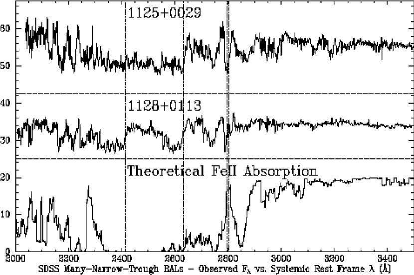
Figure 26: Comparison of SDSS 1125+0029 and SDSS 1128+0113 (each smoothed by a 3-pixel boxcar) to a theoretical Fe ii absorption spectrum constructed using data from Verner et al. (1999). Note that a covering factor of unity has been assumed for the theoretical spectrum but that the objects have partial covering, so that even saturated troughs do not reach zero flux. The dotted vertical lines show the positions of the red ends of the strong Fe ii multiplets at 2414 (UV2) and 2632 Å (UV1) plus the Mg ii doublet. There is no strong narrow Fe ii trough near 2820 Å in the theoretical spectrum which could explain the apparent longward-of-systemic Mg ii absorption.

Could the longward-of-systemic troughs be due to Fe ii absorption? This could be the case if Fe ii transitions exist between 2820 Å to 2800 Å. To test this possibility, we have used the Fe ii line lists of Verner et al. (1999) to construct a toy model of expected Fe ii absorption at the systemic redshift. We use only the Einstein A coefficients to estimate the strength of each line, thus assuming that all levels are equally populated. In reality, the higher levels which might give rise to absorption near Mg ii will be less populated than we assume, and thus the strength of such absorption lower. We created a toy absorption spectrum equal to exp($-S$), where $S$ is the arbitrarily normalized line strength ‘spectrum’, smoothed by the spectral resolution. Figure 26 compares this theoretical spectrum to the two objects in question. There is no strong narrow Fe ii trough near 2820 Å which could explain the apparent longward-of-systemic Mg ii absorption. Blueshifted absorption from Fe ii UV195,196 at 2855 Å cannot explain it either: there is no corresponding blueshifted Fe ii $\lambda$2750 Å absorption at $\sim$2695$-$2715 Å in SDSS 1125+0029, and no corresponding strong blueshifted Mg ii absorption at $\sim$2745$-$2765 Å in SDSS 1128+0113.

The only previously recognized case of a possible longward-of-systemic BAL trough, UN J1053$-$0058 (Brotherton et al. 1998a), has C iv, Al iii and Mg ii troughs extending $\sim$1500 km s^-1 longward of the C iii] redshift. However, this redshift could be biased because C iii] $\lambda$1908 can be blended with emission from Al iii $\lambda\lambda$1854,1862, Si iii] $\lambda$1892 and Fe iii UV34,61,68. It is also possible that C iii] is shifted shortward of the systemic redshift in this object: two of eighteen quasars studied by McIntosh et al. (1999) have C iii] shifted $>$1000 km s^-1 shortward of [O iii]. A literature search uncovered one previously unrecognized possible longward-of-systemic trough: the mini-BAL in 3C 288.1 (Hamann, Netzer, & Shields 2000), which lies within $\pm$1000 km s^-1 of the broad emission line $z\simeq 0.961$. A narrow-line $z$ is clearly needed for both these objects.

An indisputable host galaxy redshift for SDSS 1128+0113 and detailed Fe ii absorption line modeling for it and SDSS 1125+0029 are needed to firmly rule out other possibilities, but the simplest explanation seems to be that the BAL troughs in these objects extend longward of the systemic host galaxy redshifts.

6.5.1 Some Possible Explanations for Longward-of-Systemic BAL Troughs

Infalling gas crossing our line of sight would produce absorption longward of the systemic redshift. If the gas is in individual clouds, high-resolution spectra should show that the apparently smooth troughs around the systemic redshifts in these objects break up into narrow absorption lines. If the gas is not in individual clouds, then both a low-ionization inflow and a low-ionization outflow are present. The inflow must be optically thick and have the same maximum local covering factor as the outflow, since the absorption at $z>z_{sys}$ joins up smoothly to that at $z<z_{sys}$ both in Mg ii and in Fe ii lines with much lower optical depths. Williams et al. (1999) show that inflows and outflows with velocities and possibly column densities comparable to those observed here can coexist in the central regions of AGN. The gas in the flows seen in their isothermal models is too highly ionized to produce the absorption seen here, but it remains to be seen if more refined models explicitly including the thermal balance of the gas can reproduce the observations.

The longward troughs might be due to a freely expanding outflow. The problem with this is that the maximum trough velocities shortward and longward of the systemic $z$ are roughly equal. The free expansion velocity is therefore much larger than the outflow velocity, leaving us with no explanation for what has accelerated the gas to such high velocities. A similar problem arises in the model of Scoville & Norman (1995). In that model BALs arise in debris trails from mass-losing stars in the nuclear star cluster, but the observed redshifted velocities in these objects are larger than the central velocity dispersions of any galaxy.

We might instead be viewing an outflow that arises from a distribution of clouds with a substantial virial velocity dispersion. In this picture, the extent of the absorption longward of the systemic redshift would be the same for troughs of different ionization, but the absorption shortward would depend on the ionization present at different velocities in the outflow, and so could be different for different ions. (Recall that high-ionization absorption typically extends to higher terminal velocities than low-ionization absorption.) To keep the velocity dispersion $\sigma$ from being too large in this case, the clouds must be located far away from the quasar. Assuming a $10^{8}M_{\odot}$ black hole and an isotropic velocity field, a distance of $5\times 10^{17}$ cm (7 light-months) is required to match the observed $\sigma_{LOS}=\sigma/\sqrt{3}\sim 1000$ km s^-1. An isotropic velocity dispersion for the cloud population seems most likely: the clouds cannot all be on plunging orbits as they would soon be destroyed after approaching too close to the central engine, and it is unlikely that they have a disklike distribution given the observed radial velocity dispersion. An isotropic velocity dispersion implies that the clouds have a global covering factor of essentially unity, which has been predicted for at least some LoBALs from other considerations (Canalizo & Stockton 2001). However, longward-of-systemic absorption should not be rare in this model. Its apparent rarity must be attributed to the difficulty of obtaining narrow-line redshifts given the weakness of [O iii] in LoBALs (Boroson & Meyers 1992). It is also not obvious if this model can explain why BAL troughs do not show variability in velocity as well as amplitude, or if it can explain the similar trough shapes in our two objects, which the next model we discuss might.

6.5.2 An Extended Continuum Source Seen Through a Rotation Dominated Disk Wind?

A possibly more promising explanation arises from geometry and rotation. A wind arising from a rotating accretion disk will share the rotation velocity of the disk, and in fact the tangential velocity may initially dominate the vertical and radial velocities. If we have a grazing line of sight to such an accretion disk which passes through a section of the wind where the velocity is predominantly rotational, and if the continuum source is no more than an order of magnitude smaller than the inner radius of the wind, the wind can have both approaching and receding velocities along our line of sight (cf. (Proga et al. 2002), where this possibility is mentioned for disk winds in cataclysmic variables).

This is demonstrated in Figure 27a, which shows a top view of such a disk. The inner edge of the wind is at radius $R$, and $\phi$ is the angular coordinate along the surface of the disk measured from our line of sight. The continuum at some absorption wavelength of interest is assumed to arise predominantly from radii $r<r_{max}$, since the disk beyond $r_{max}$ will be too cool to contribute significant emission at that wavelength. A wind element at ($R,\phi$) will have velocity $v_{LOS}$ and will absorb continuum emission from a region of length $L$ at that velocity. As seen in the Figure, $v_{LOS}$ can be redshifted if the rotational velocity dominates.

Figure 27b is a side view of one quadrant of the same disk. The disk has inclination angle $i$ measured from the line of sight toward the disk normal; i.e., $i=90$° for an edge-on disk and $i=67\arcdeg$ in Figure 27b. The wind opening angle is $\lambda$, measured in the $\theta$ direction from the plane of the disk. The disk, which is optically thick, is shown as the heavy line running diagonally across the entire plot. The wind arises at radius $R$ (and beyond), and fills at most the region outlined by the three thick lines. The wind may initially be dominated by its vertical velocity $v_{z}$, but at the terminal opening angle $\lambda$ the radial velocity $v_{rad}\gg v_{z}$ and the wind has essentially no vertical velocity component.

The wind can absorb flux from a continuum emitting region of size $r_{max}$ only if the wind rises far enough above the disk to be seen in projection against this region before becoming purely radial. Geometrically, $i$ must be large enough to satisfy the inequality

$$R\cos(i)-r_{max}\cos(i)\leq R\tan(\lambda)\sin(i)$$ (3)

which simplifies to

$$1-\tan(i)\tan(\lambda)\leq r_{max}/R$$ (4)

This constraint is a weak one which will be satisfied for any line of sight to the black hole which passes through the BAL wind. However, if the continuum source is extended enough, this constraint can also be satisfied for some inclination angles $i<90\arcdeg-\lambda$ where the line of sight to the black hole itself does not pass through the wind. (This complicates the conversion from wind covering factor to BAL covering factor, but provides an additional way to achieve partial covering of the continuum source.)

For disks with inclination angles $i$ large enough to satisfy Equation 4, the wind will be seen in absorption over a range of velocities given by

$$v_{LOS}=v_{rot}\sin(i)\sin(\phi)+v_{z}\cos(i)+[0,v_{rad}]\times[\cos(i),\sin(i+\lambda)]\times\cos(\phi)$$ (5)

for $-\Phi<\phi<\Phi$. Here $v_{rot}$ is the rotational velocity at $R$, $\Phi$ is the maximum tangential angle $\phi$ for which the wind shadows the continuum emission region ($\sin\Phi=r_{max}/R$), and $v_{z}$ refers only to the initial vertical velocity of the wind and not the component of the radial velocity $v_{rad}$ perpendicular to the disk. The terms in brackets indicate possible ranges. Acceleration will produce a range of radial velocities $v_{rad}(\theta)$ as wind elements move from $\theta=0$ to $\theta=\lambda$, with $v_{rad}(0)=0$ for an initially vertical wind. Geometry produces a range of line of sight projection factors for those radial velocities, from cos($i$) at $\theta=0$ to sin($i$$+$$\lambda$) at $\theta=\lambda$, passing through a maximum of unity if $i+\lambda>90\arcdeg$.

The $v_{rot}$ term in Equation 5 is the only one which can be negative. This equation demonstrates that longward-of-systemic absorption can occur for lines of sight where the wind velocity is dominantly rotational. The maximum longward-of-systemic velocity will occur if our line of sight passes through BAL gas which has not yet experienced significant radial acceleration.

6.5.3 Consistency with Literature Models

The quasar models of Murray et al. (Murray & Chiang 1998, and references therein) and Elvis (2000) both incorporate disk winds, and so longward-of-systemic absorption is possible in both scenarios. For both these models, we can estimate the maximum possible redshifted velocity and the maximum angle over which longward-of-systemic absorption might be seen by assuming a purely vertical flow with $v_{rad}=0$. We also assume Keplerian rotation ($v_{rot}=\sqrt{2GM_{BH}/R}$) and that the 2800 Å continuum arises from the accretion disk at radii out to $r_{max}=5.7\times 10^{15}$ cm (pp. 37 and 45 of Peterson 1997). This is a conservative assumption because we use the radius of peak emission at 2800 Å as $r_{max}$, rather than the largest radius at which significant 2800 Å emission is produced, and so we slightly underestimate $r_{max}/R$.

In the Elvis model, the wind begins vertically and slowly becomes radial, forming a funnel with a effective wind opening angle of $\lambda$=27°. Elvis (2000) gives $R=10^{16}$ cm for NGC 5548, which has $M_{BH}=5.9\pm 2.5~{}10^{7}M_{\odot}$ (Peterson & Wandel 2000). We take $R=1.5\times 10^{16}$ cm since we are primarily concerned with low-ionization absorption, which in this model arises from radii up to twice as large as that of the high-ionization absorption (Figure 5 of Elvis 2000). Thus $v_{rot}$=8800 km s^-1 and $\sin\Phi=(r_{max}/R)=0.285$. Equation 4 then requires $i>48$° for shadowing to occur; however, the wind is only visible for $i>63$° since the radial part of the flow is optically thick. Using $v_{z}$=6000 km s^-1 (§3.2 of Elvis 2000), Equation 5 gives $v_{LOS}=\pm 2500$sin($i$)+6000cos($i$) km s^-1. This yields possible line of sight velocity ranges from $500<v_{LOS}<5000$ km s^-1 for $i=63\arcdeg$ to $-2400<v_{LOS}<2600$ km s^-1 for $i=89\arcdeg$ (assuming a disk opening angle of 1°). The maximum negative velocity and the range of velocities for $i=89\arcdeg$ are only a factor of 1.3–2 higher than the observed velocities in the two SDSS quasars with longward-of-systemic absorption.

In the Murray et al. model, the wind streamlines rapidly become purely radial, resulting in a wind opening angle of only $\lambda$=6°. For $M_{BH}=10^{8}M_{\odot}$ the wind begins at $R=3.7\times 10^{16}$ cm. Thus, $\sin\Phi=r_{max}/R=0.154$, and shadowing occurs for $i>83$°. We adopt $v_{z}$=5000 km s^-1 since Murray et al. (1995) state that the wind streamlines are more vertical than radial at such outflow velocities. Equation 5 then yields $v_{LOS}=\pm$1300sin($i$)+5000cos($i$) km s^-1. With a disk opening angle of 1° (Murray et al. 1995), the ranges of possible velocities range from $-600<v_{LOS}<1900$ km s^-1 for $i=83\arcdeg$ to $-1200<v_{LOS}<1300$ km s^-1 for $i=89\arcdeg$. The $i=89\arcdeg$ numbers are in good agreement with the observations of the two SDSS quasars.

Thus, both these models produce estimated ranges of absorption velocities which are qualitatively consistent with those observed in the two SDSS quasars with longward-of-systemic absorption. However, are the $M_{BH}$ values used in those estimates ($5.9-10\times 10^{7}~{}M_{\odot}$) appropriate for those quasars? Converting the two quasars’ absolute $i^{*}$ magnitudes to $M_{B}$ using $M_{B}\simeq M_{i^{*}}+0.35$, adopting a bolometric correction of $-2.7\pm 0.4$ magnitudes and assuming a typical quasar value of $L/L_{edd}=0.1$ (McLeod, Rieke, & Storrie-Lombardi 1999), we estimate $M_{BH}$ values of 4.2 and 3.3 $\times 10^{7}~{}M_{\odot}$ for the two SDSS quasars. This is within a factor of two to three of the values used in the estimates, which is adequate given the uncertainties.

Finally, we note that the de Kool & Begelman (1995) magnetically confined disk wind model cannot explain longward-of-systemic absorption. Their wind arises so far from the continuum source that the source no longer appears appreciably extended. In that model $R\simeq 10^{18}$ cm, so $\sin\Phi=r_{max}/R<0.001$ and the potentially negative first term in Equation 5 is negligible.

6.5.4 Testing Our Explanation

We have shown that incorporating an extended continuum source in either the Murray et al. or Elvis disk wind models appears capable of explaining redshifted BAL absorption. Extended continuum sources are a generic result of accretion disk models, though such models are not without their problems (e.g., pp. 45-55 of Peterson 1997). Redshifted absorption requires a very nearly edge-on geometry so that the rotation-dominated base of the wind shadows much of the continuum source. Nearly edge-on geometries are of course intrinsically rare, and many such objects will be hidden by dust if accretion disks are roughly coplanar with the torii of gas and dust thought to exist at larger radii (Schmidt & Hines 1999). Thus the observed rarity of redshifted absorption troughs is to be expected. Nonetheless, other longward-of-systemic BAL troughs may have gone unrecognized due to confusion with Mg ii emission and to the scarcity of narrow-line host galaxy redshifts for BAL quasars, let alone stellar absorption-line redshifts. In particular, some strong $z_{abs}>z_{em}$ associated absorption systems in radio-loud quasars (Anderson et al. 1987) could be redshifted mini-BALs.

There are several ways of testing our model. Shorter continuum wavelengths are produced at smaller $r_{max}$ in standard disk models. Since a smaller $r_{max}$ will decrease the maximum observable redshifted velocity, troughs at shorter wavelengths should have smaller longward extents if standard disk models are correct. In fact, near-simultaneous UV-optical variability suggests that at least part of the UV-optical continuum emission is reprocessed high-energy emission (Peterson 1997, p. 48), in which case all troughs might have the same longward extents. We cannot determine which is the case from existing data. In SDSS 1125+0029 and SDSS 1128+0113 the SNR and/or resolution are insufficient to study any trough besides Mg ii, given the huge number of Fe ii and other transitions in the wavelength range observed. High-resolution data for higher-ionization transitions in the two low-redshift objects would also help test the virial velocity dispersion model. The longward-of-systemic absorption should be the same for all lines in that model, while confirmation in both objects of O-star-like absorption profiles (deepest at high outflow velocities) would be difficult to understand because the absorption profiles in different objects should be uncorrelated since the gas is on random orbits.

More detailed comparisons with the spectra might be possible if some effects we have neglected are considered (e.g., disks so thick that the disk opening angle is comparable to or greater than the wind opening angle). Elliptical and/or warped disks might be needed to explain why the observed Mg ii troughs extend farther longward of systemic than shortward; in the model presented herein any such asymmetry should be to the blue. Also, the continuum emission region may be more of an annulus than a disk, since the inner disk will be very hot and may not contribute significant emission at the wavelength in question. For a narrow annulus, the path length $L$ shadowed by the BAL flow may be smaller at $\phi=0$ than near the maxima $\phi=\pm\Phi$. Similarly, the column density through the BAL flow will have a weak minimum at $\phi=0$ if its gas density is constant with $\phi$. This may explain the local minimum in the absorption at 2800 Å in SDSS 1128+0113. Finally, limb darkening (Hubeny et al. 2000) and other radiative transfer effects (e.g., Murray & Chiang 1997) will affect the disk emission source function $S_{\nu}(\theta,\phi)$ and thus the amount of emission available for absorption by a wind element at ($R,\phi$). For example, relativistic beaming will brighten the approaching side of the disk and dim the receding side (e.g., Hubeny et al. 2000). If this effect is the dominant one and the BAL region is optically thick, the absorption profiles will be deeper at shorter wavelengths. Such profiles are seen in both low-redshift objects and possibly in SDSS 1723+5553, though in that case the shape may be due to unabsorbed broad Mg ii emission (Arav et al. 1999a). Nonetheless, if the BAL regions in these objects are probing different regions of the quasar accretion disk as a function of velocity, then they have the potential to provide powerful constraints on accretion disk models.

6.6 How Common Are Unusual BAL Quasars?

Having selected different types of unusual BAL quasars from early SDSS data, we can ask what fraction of the quasar population they form. In the redshift range $1.485<z<3.9$ where selection of both HiBALs (via C iv) and LoBALs (via Mg ii or Al iii) is possible, there are 1807 quasars in the SDSS EDR quasar sample (Schneider et al. 2002). In this redshift range our sample of BAL quasars (Reichard et al. 2002) includes 284-306 BAL quasars (15.7%-16.9%) by the AI definition, or 181-219 (10.0%-12.1%) by the BI definition. The lower numbers are firm figures, while the higher numbers include borderline cases (low SNR, preliminary indices less than required by only 1$\sigma$, etc.) For comparison, at somewhat lower average redshifts the LBQS survey finds a BAL quasar fraction of 8-11% (Weymann 1997) and the FBQS survey 14-18% (Becker et al. 2000). The number of LoBALs at $1.485<z<3.9$ in the SDSS EDR is 28 by the AI definition or 24.5 (the 0.5 is a borderline case) by the BI definition. Thus LoBALs make up 1.5$\pm$0.4% of the SDSS EDR sample at $1.485<z<3.9$, in agreement with canonical numbers (§1).

There are four FeLoBALs in the EDR in this redshift range, and three or four more at lower $z$. There are two unusual FeLoBALs in the EDR in this redshift range: SDSS 1723+5553 (§5.1) and SDSS 1730+5850 (§5.2), and two or three more at lower $z$: SDSS 1125+0029 (§5.1), SDSS 0300+0048 (§5.2), and possibly SDSS 0105$-$0033 (§5.5). The other unusual BAL quasars in the EDR are all at $z<1.485$: SDSS 1214$-$0001 (§5.4), SDSS 1453+0029 and SDSS 0127+0114 (§5.3.2). Thus, preliminary numbers from the (incomplete) SDSS EDR quasar sample indicate that unusual LoBAL quasars are about equal in number to FeLoBALs and that 50% of all FeLoBALs fall into one of our categories of unusual objects. Since most of these unusual BAL quasars are considerably redder than the targets of most quasar surveys, and since FeLoBALs comprise $\sim$15% of LoBALs, most previous samples of LoBAL quasars are likely to be incomplete by $\gtrsim$15%. This incompleteness would have little effect on the overall numbers of quasars in any survey, since even a factor of two increase in the number of LoBALs would translate to only a few percent more quasars overall, but it has probably biased our view of the range of column densities and velocity widths spanned by BAL outflows.

Note that our numbers are in agreement with Meusinger & Brunzendorf (2001), who used an optical variability and zero proper motion survey to limit the fraction of ‘unusual’ quasars to $<5$% for $B\leq 19.7$.

7 Summary and Conclusions

We have presented over twenty unusual broad absorption line quasars selected from $\lesssim$15% of the eventual Sloan Digital Sky Survey database. These objects confirm that several populations of BAL quasars with unusual properties exist, and that the range of parameter space spanned by BAL outflows is larger than previously realized. Even so, these objects are all low-ionization BAL quasars (LoBALs). A corresponding population of HiBALs with extensive absorption from only high-ionization transitions could exist, but the rest-frame optical-UV region probed by SDSS spectra is not very sensitive to such absorption. The total population of unusual LoBAL quasars is at least as extensive as that of LoBAL quasars with absorption from excited-state Fe ii or Fe iii — about 15% of LoBALs — and about half of such FeLoBALs qualify as unusual (§6.6). Unusual BAL quasars are thus not an enormous population, but their properties may provide more stringent tests of BAL outflow models than do the more numerous ‘normal’ BAL quasars.

The unusual BAL quasars we have found to date can be divided into four or five categories.
$\bullet$ Two objects with many narrow troughs show Mg ii absorption extending longward of their systemic host galaxy redshifts by $\sim$1200 km s^-1. We favor an explanation where this is due to absorption of an extended continuum source by the rotation-dominated base of a disk wind, but other explanations are possible (§6.5).
$\bullet$ Five objects have absorption which removes an unprecedented $\sim$90% of all flux shortward of Mg ii (§5.2). The absorption in one of them has varied across the ultraviolet with an amplitude and rate of change among the greatest ever seen in BAL quasars (§6.4). This same object may also show broad H$\beta$ absorption (§5.2.5). These objects may not be fundamentally new, but they do show that low-ionization absorption can have outflow velocities as large as any ever seen in high-ionization lines.
$\bullet$ Numerous heavily reddened BAL quasars have been found, including two reddened mini-BALs with very strong Fe ii emission (§5.3.2). The five reddest objects are reddened by $E(B-V)$ $\simeq 0.5$ (§5.3.3), and in two of them we find strong evidence that the extinction curve is even steeper than that of the SMC (§6.3.1).
$\bullet$ We have found at least one object with absorption from Fe iii but not Fe ii, which may be due to an unusually high column density of moderately high-ionization BAL gas (§5.4). Also, the relative strengths of excited term Fe iii absorption in these objects is different than in most BALs with Fe iii absorption, and cannot be achieved in LTE, so some sort of resonance must be at work (§6.2).
$\bullet$ Lastly, we have found two luminous, probably reddened high-redshift objects which may be BAL quasars whose troughs partially cover different regions of the continuum source as a function of velocity (§6.1).

Many of these objects show absorption from neutral atoms such as Mg i and He i, which can be used to constrain the density and ionization in the BAL gas. Sometimes the distance of the BAL gas from the central ionizing source can also be constrained, assuming photoionization equilibrium with that source (Arav et al. 2001a). We have presented three new BAL quasars with He i absorption (Table 2), and possibly two more (SDSS 1730+5850 and SDSS 0318$-$0600). Also, all five of our overlapping-trough BAL quasars (including SDSS 1730+5850) have Mg i absorption, and SDSS 0318$-$0600 may have it as well. This substantially increases the number of objects known to exhibit absorption in these valuable transitions.

We close with a mention of some potentially fruitful avenues of research on these unusual LoBAL quasars. Near-IR spectroscopy and spectropolarimetry of all these objects would help determine if they fit into a geometrical ‘dusty torus’ picture of BAL quasars (Schmidt & Hines 1999) or whether they represent an early ‘cocoon’ phase in the evolution of individual quasars (Becker et al. 2000). High resolution spectroscopy of the longward-of-systemic absorption troughs in SDSS 1125+0029 and SDSS 1128+0113 could differentiate between several models for BAL outflows. Despite the broad and blended absorption in overlapping-trough BAL quasars, targeted high resolution spectroscopy of Ca ii in SDSS 0300+0048 and He i in SDSS 1730+5850 might determine if the column densities as well as the outflow velocities are very large in these objects. Photoionization modeling including detailed treatment of Fe ii and Fe iii may be needed to understand Fe iii-dominant BAL quasars, particularly the resonance at work in at least SDSS 2215$-$0045. Lastly, detailed modeling of disk winds and turbulent outflows is needed to determine if such models can explain the wide range of properties seen in these objects, and where such models need to be revised if they cannot.

Appendix A The Balnicity Index Reconsidered

A.1 The Standard Balnicity Index (BI)

Weymann et al. (1991) defined a ‘balnicity index’ or BI with the aim of providing a continuous measure of the strength of the broad absorption while excluding intervening and associated absorption systems. The most physically relevant quantity for gauging BAL strength is the column density in the BAL system(s), but this can be measured only in some objects, and even then requires high-resolution spectroscopy and detailed modeling. The BI is a useful substitute, being an observable quantity calculable from low-resolution data.

The BI is calculated from C iv (treating it as a single transition at 1549 Å) as follows. Define the quasar $z$ using Mg ii, C iii], or C iv (in order of preference), fit a continuum between Si iv/O iv] and C iv, and interpolate over non-C iv absorption in that wavelength region. Between 3000 km s^-1 and 25000 km s^-1 shortward of 1549 Å at the systemic redshift, measure the modified equivalent width (in km s^-1) of the portions of contiguous absorption troughs exceeding 2000 km s^-1 in velocity. The equivalent width is ‘modified’ because ‘absorption’ is defined as only those parts of the troughs which dip at least 10% below the adopted continuum level. Thus the maximum BI is 20000 km s^-1.

The criterion of a 10% dip for absorption was established to ensure that false BAL troughs are not identified by placing the continuum too high; the 2000 km s^-1 contiguity condition to avoid strong intervening narrow-line absorption complexes; the 3000 km s^-1 red integration limit to avoid strong associated narrow-line C iv $\lambda\lambda$1548,1550 complexes; and the 25000 km s^-1 blue integration limit to avoid confusion with Si iv/O iv] $\lambda$1400 emission and Si iv BAL troughs.

A.2 The Ideal Balnicity Index

It is worth considering exactly what the ‘ideal’ balnicity index is that we are trying to measure. The ideal BI would be found by measuring the standard equivalent width (in rest-frame km s^-1 at the quasar systemic redshift) of all confirmed C iv BAL troughs shortward of the systemic redshift.

The ideal BI would have the following advantages over the standard BI:
$\bullet$ It would not exclude BAL quasars with broad, shallow troughs such as UM 660 (Turnshek 1988).
$\bullet$ It would not exclude BAL troughs within 3000 km s^-1 of the systemic velocity.
$\bullet$ It would not exclude ‘mini-BAL’ troughs (Hamann 2000) which have contiguous width $<$2000 km s^-1 but otherwise share all the characteristics of BAL troughs.
$\bullet$ It can be calculated for high-velocity BAL quasars with troughs that extend to $>$25000 km s^-1 but are not confused with troughs from other transitions (e.g., PG 2302+029; Jannuzi et al. 1996),

The drawback of the ideal BI, of course, is that it requires exact knowledge of the quasar’s systemic velocity and continuum shape, and of which absorption troughs arise in BAL outflows as opposed to being intervening systems (of C iv or other species) or intrinsic systems unrelated to the BAL outflow.

A.3 A Suggested Compromise: The Intrinsic Absorption Line Strength Index (AI)

Weymann et al. (1991) note that “…better resolution data, coupled with a more refined definition of balnicity, are required to treat … borderline cases.” Since SDSS spectra have a wavelength resolution good enough to identify many intervening absorption systems, we have defined a provisional revised balnicity index that makes more optimal use of SDSS data. Since our goal is to measure the strength of all intrinsic absorption, not just broad intrinsic absorption, we refer to this revised balnicity index as the intrinsic absorption index or AI. The final values of some of the parameters used in the AI may change based on the results of ongoing detailed studies of SDSS BAL quasars, but the general framework for choosing those parameters is presented here. The specific issues addressed in the definition of the AI are as follows.

The systemic velocity:

In some objects the Mg ii emission line $z$ is uncertain, let alone that of C iii] or C iv. We adopt the host galaxy stellar absorption-line redshift whenever possible; otherwise, we follow Vanden Berk et al. (2001) and adopt as systemic the redshift of [O iii] $\lambda$5008 (vacuum $\lambda$), or [O ii] $\lambda\lambda$3727,3729 if [O iii] is unavailable. We correct the $z$ measured from other lines to this systemic $z$ using the velocity shift for that line as measured in the SDSS composite quasar (Vanden Berk et al. 2001). These velocity shifts may change slightly as more objects are added to this composite, but a greater concern to be addressed when more quasars are in hand is whether different quasar subtypes have different velocity shifts.

The continuum shape:

We begin with a fifth-order polynomial fit to the windows discussed in Weymann et al. (1991): 1575-1625 Å, 1800-1820 Å, 1975-2000 Å, 2140-2155 Å, 2190-2200 Å, 2240-2255 Å, 2665-2695 Å plus a window longward of Mg ii. The windows do not always sample the continuum, so they are adjusted where necessary to reach an acceptable final fit. Note that in most cases it is not possible to accurately include broad emission lines in the fit, and so the depth of the absorption will be underestimated where the absorption overlaps in wavelength with the broad emission. It may be possible to automate the continuum determination for even heavily absorbed BAL quasars by comparison with weaker BAL quasars as well as non-BAL quasars, perhaps along the lines of Connolly & Szalay (1999). It may also be worthwhile to use a 3$\sigma$ significance criterion for determining the starting and ending points of absorption troughs, which would also allow the minimum detectable AI for a given spectrum to be defined without requiring an arbitrary 10% dip below the continuum level. For now, we use the same modified equivalent width as the BI since empirically we find it reduces the identification of random fluctuations as BAL troughs. A 10% systematic uncertainty in continuum placement is reasonable in most cases, so we adopt that as a characteristic systematic error until a larger number of SDSS quasar spectra are available to study the issue statistically.

Intrinsic vs. Intervening Absorption:

Hamann (2000) points out that mini-BAL troughs and confirmed intrinsic narrow absorption line (NAL) troughs are found over a range of ejection velocities comparable to those of BAL troughs. We wish to measure the strength of such intrinsic, outflowing systems while ignoring intervening systems and associated systems from gas in or near the quasar host galaxy and its environs. Confirmation that a given system is intrinsic requires detection of nonblack saturation, time variability on timescales of years, well-resolved smooth profiles which are broad compared to thermal line widths, densities $>$100 cm^-3 inferred from excited-state absorption, or possibly very high metallicities (e.g., Hamann et al. 1997). Most of these measurements are beyond the capabilities of SDSS spectra, but with an instrumental resolution of $\simeq 150$ km s^-1 we can resolve individual narrow C iv and Mg ii systems (doublet separations 498 km s^-1 and 769 km s^-1, respectively). Thus in many cases we will be able to directly determine whether an absorption feature $<$2000 km s^-1 wide is a BAL trough or a complex of narrow absorption systems. For the AI we therefore adopt a 450 km s^-1 contiguity criterion instead of the 2000 km s^-1 criterion used for the BI. We also slightly revise the definition of contiguous to include all absorption from troughs $\geq 450$ km s^-1 wide, rather than only the absorption beyond the first 2000 km s^-1. We feel the odds of finding non-BAL systems in such close proximity to BAL systems are small enough to make an occasional overestimate of the AI acceptable. However, we do consider the 450 km s^-1 value of the contiguity criterion to be preliminary and subject to revision pending more detailed future studies of SDSS BAL quasars.

Which Transitions To Use:

The AI can be calculated for any transition, but for consistency with the BI we use C iv whenever possible. When another transition is used, it should be noted in parentheses: e.g., AI(Mg ii). For objects with no C iv data, Si iv is the best alternative for HiBALs, and Mg ii or Al iii for LoBALs. Mg ii or Al iii absorption can also be used for objects where the continuum around C iv is very difficult to estimate. Low-ionization troughs such as Mg ii and Al iii are typically narrower than high-ionization troughs, but eventually it may be possible to correct for this effect statistically.

Definition of the AI:

After defining the systemic redshift and the continuum level and interpolating over all absorption features besides the relevant trough, the AI and statistical uncertainty are calculated as

$${\rm AI}=\int_{0}^{(25,000)}[1-f(v)/0.9]~{}C^{\prime}~{}dv$$ (A1)

$$\sigma_{\rm AI}^{2}=\int_{0}^{(25,000)}(\sigma_{f(v)}/0.9)^{2}~{}C^{\prime}~{}dv$$ (A2)

where $f(v)$ and $\sigma_{f(v)}$ are the normalized flux and uncertainty (unsmoothed whenever possible) as a function of velocity in km s^-1 from the systemic $z$. Thus, like the BI, the AI has units of km s^-1. The integral begins at the systemic redshift ($v=0$) at the wavelength of the shortest-wavelength line of any multiplet involved (e.g., 1548.20 Å for C iv or 2796.35 Å for Mg ii). The integral extends beyond the highest velocity intrinsic C iv system, but in practice the maximum velocity will often be limited by confusion with Si iv troughs at 25000 km s^-1, so we have noted this in parentheses as a typical limit. The value of $C^{\prime}$ is unity in contiguous intervals of width 450 km s^-1 or greater where the quantity in brackets is everywhere positive; otherwise $C^{\prime}=0$. The AI is therefore linear from 450 km s^-1 to $>$25,000 km s^-1, the latter being a lower limit when the C iv absorption appears to extend beyond Si iv but is confused with the Si iv BAL troughs. The AI can also be extended to $<$450 km s^-1 using higher resolution spectra. Finally, the presence of BAL troughs longward of the systemic redshift (§6.5.2) can be indicated with a superscripted +, e.g., 3000⁺. If our explanation for this phenomenon is correct (§6.5), the AI in such cases should still be measured from the systemic redshift.

In practice the statistical uncertainty is dwarfed by the systematic uncertainty in the continuum placement. Nonetheless we quote errors for the AI since they are useful for marginal objects, and since detailed study of large BAL and non-BAL quasar samples may eventually reduce the systematic uncertainty to a level comparable to the statistical uncertainty.

IRAF and SM code for determining a continuum, normalizing a spectrum by it, and calculating its AI or BI value is available, along with all spectra of unusual BAL quasars presented in this paper (§4), from the contributed data section of the SDSS Archive at http://archive.stsci.edu/sdss/.

Table 1: Transitions with $\lambda\geq 1215$ Å Seen to Date in BAL Quasars

		Ionization Potentials for…		BAL	Frequency
Transition	Vacuum Wavelength (Multiplet)	Creation	Destruction	Subtype	in Subtype
Ly$\alpha$	1215.67	0.0	13.6	Hi	common
N v	1238.82,1242.80	77.5	97.9	Hi	common
Si ii	1260.42 (UV4)	8.1	16.3	Lo	unusual
Si ii*	1264.74,1265.00 (UV4)	(0.05)	16.3	Lo	rare
O i	1302.17	0.0	13.6	Lo	unusual
Si ii	1304.37 (UV3)	8.1	16.3	Lo	unusual
Si ii*	1309.28 (UV3)	(0.05)	16.3	Lo	rare
C ii	1334.53 (UV1)	11.3	24.4	Lo	unusual
C ii*	1335.66,1335.71 (UV1)	(0.01)	24.4	Lo	rare
Si iv	1393.76,1402.77	33.5	45.1	Hi	common
Si ii	1526.73 (UV2)	8.1	16.3	Lo	unusual
Si ii*	1533.43 (UV2)	(0.05)	16.3	Lo	rare
C iv	1548.20,1550.77	47.9	64.5	Hi	(defines)
Al ii	1670.79	6.0	18.8	Lo	unusual
Ni ii(*)	1709.6,1741.5,1751.9,1773.9 (UV5,4,3)	7.6	18.2	FeLo?	rare
P i	1774.95,1782.83,1787.65 (UV1)	0	10.5	FeLo?	rare
Si ii	1808.01 (UV1)	8.1	16.3	Lo	unusual
Al iii	1854.72,1862.79	18.8	28.4	Lo	common
Fe iii	1895.46,1914.06,1926.30 (UV34)	(3.7)	30.7	FeLo	common
Mg i	2026.48	0.0	7.6	FeLo?	rare
Zn ii	2026.14,2062.66	9.4	18.0	FeLo?	rare
Cr ii	2056.25,2062.23,2066.16	6.8	16.5	FeLo?	rare
Fe iii	2062.21,2068.90,2079.65 (UV48)	(5.1)	30.7	FeLo	unusual
Fe i	2167.45 (UV21)	0.0	7.9	FeLo?	rare
Ni ii	2225 (UV12,13)	7.6	18.2	FeLo?	rare
Co ii	2300 (UV9)	7.9	17.1	FeLo?	rare
Ni ii	2300 (UV11)	7.6	18.2	FeLo?	rare
Mn ii	2576.88,2594.50,2606.46	7.4	15.6	FeLo?	rare
Cr ii	2680 (UV7,8)	(1.48-1.55)	16.5	FeLo?	rare
Mg ii	2796.35,2803.53	7.6	15.0	Lo	(defines)
Mg i	2852.96	0.0	7.6	FeLo?	rare
Cr ii	2860 (UV5)	(1.48-1.55)	16.5	FeLo?	rare
He i	2945.97,3188.67,3889.74	(19.8)	24.6	Lo	rare
O iii	3133.70	(36.9)	54.9	Lo	rare
Ca ii	3934.78,3969.59	6.1	11.9	Lo	rare
Na i	5891.58,5897.56	0.0	5.1	Lo	rare
Fe ii Multiplets
Fe ii	1570 (UV44,45,46)	(0.15-0.25)	16.2	FeLo	rare
Fe ii(*)	1608.45 (UV8)	7.9	16.2	Lo	rare
Fe ii	1710 (UV38)	(0.23-0.38)	16.2	FeLo	rare
Fe ii]	1781.70 (UV67)	(1.07)	16.2	FeLo	rare
Fe ii	1785.27,1786.75,1787.996 (UV191)	(2.88)	16.2	FeLo	rare
Fe ii	2151.8,2153.0,2177.7 (UV106)	(2.27-2.33)	16.2	FeLo	rare
Fe ii	2164.34,2173.72 (UV79)	(1.66-1.69)	16.2	Lo	unusual
Fe ii(*)	2249.88 (UV5)	7.9	16.2	Lo	unusual
Fe ii(*)	2260.78 (UV4)	7.9	16.2	Lo	unusual
Fe ii	2298.93 (UV133)	(2.63)	16.2	FeLo	rare
Fe ii(*)	2344.21 (UV3)	7.9	16.2	Lo	unusual
Fe ii(*)	2374.46,2382.77 (UV2)	7.9	16.2	Lo	unusual
Fe ii	2382.90,2388.39 (UV117)	(2.51-2.57)	16.2	FeLo	rare
Fe ii*	2400,2600 (UV2,1)	(0.05-0.12)	16.2	FeLo	(defines)
Fe ii	2420 (UV35,36)	(0.23-0.39)	16.2	FeLo	rare
Fe ii	2460 (UV209)	(3.14-3.22)	16.2	FeLo	rare
Fe ii	2580 (UV64)	(0.98-1.09)	16.2	FeLo	rare
Fe ii(*)	2586.65,2600.17 (UV1)	7.9	16.2	Lo	unusual
Fe ii	2750 (UV62,UV63)	(0.98-1.09)	16.2	FeLo	common
Fe ii	2880 (UV61)	(0.98-1.07)	16.2	FeLo	rare
Fe ii	2950 (UV60)	(0.98-1.09)	16.2	FeLo	rare
Fe ii	2985 (UV78)	(1.66-1.72)	16.2	FeLo	rare
Fe ii	3180 (Opt7)	(1.66-1.72)	16.2	FeLo	rare
Fe ii	3200 (Opt6)	(1.66-1.72)	16.2	FeLo	rare

Note. — We list only firmly identified transitions seen in one or more BAL quasars (in papers up to, but not including, de Kool et al. 2002). Thus, for example, we do not list Cr ii UV6 or Fe ii UV144-149,158-165 absorption even though at least some of those multiplets are certainly present in SDSS 1125+0029 because we cannot verify any individual lines from those multiplets in our low-resolution spectra. Under Transitions, ‘*’ refers to excited level absorption from ground term multiplets, and ‘(*)’ denotes ground term multiplets where absorption from both ground and excited levels has been seen (however, the BAL Subtype refers only to the ground level lines). Ionization Potentials are given in eV. Wavelengths given only to the nearest Å refer to multiplet absorption. Under ‘BAL Subtype’, FeLo? means that the transitions have only been seen in FeLoBALs to date, but that there is no a priori reason they could not be seen in LoBALs. Transitions seen in HiBALs are also seen in the other two subtypes, and transitions seen in LoBALs are also seen in FeLoBALs. The ‘Frequency in Subtype’ entries (common, unusual, or rare) refer to the frequency within the listed BAL subtype. ‘Defines’ mean that the presence of that transition defines that BAL subtype: C iv for HiBALs, Mg ii for LoBALs, and Fe ii* (excited Fe ii) for FeLoBALs. Note that absorption from any excited level or term of Fe ii qualifies the object as a FeLoBAL; we explicitly list only the UV1 and UV2 multiplets as Fe ii* simply because they contain the strongest excited-level transitions.

Table 2: SDSS Unusual BAL Quasars

J2000	Redshift	BAL	$BI$,	$AI\pm\sigma_{AI}$,		Target	20cm,							Galactic
Coordinates	$z$$\pm$$\sigma_{z}$	Type	km s-1	km s-1	EDR	Code	mJy	$M_{i^{*}}$	$u^{*}\pm\sigma_{u^{*}}$	$g^{*}\pm\sigma_{g^{*}}$	$r^{*}\pm\sigma_{r^{*}}$	$i^{*}\pm\sigma_{i^{*}}$	$z^{*}\pm\sigma_{z^{*}}$	$E$$($$B$$-$$V$$)$
010540.75$-$003314.0	1.1788$\pm$0.0001	?	0	0	Y	11011	4.59	$-$26.59	20.42$\pm$0.06	19.29$\pm$0.02	18.01$\pm$0.02	17.69$\pm$0.01	17.41$\pm$0.03	0.034
012702.52$+$011412.5	1.1571$\pm$0.0002	red,He i	0	50$\pm$1	Y	01000	1.06	$-$26.84	20.40$\pm$0.07	18.92$\pm$0.02	17.87$\pm$0.02	17.38$\pm$0.02	17.08$\pm$0.03	0.027
014905.28$-$011404.9	2.10$\pm$0.01	Fe iii?	56	2930$\pm$5	Y	10000	$<$1.05	$-$25.76	23.14$\pm$0.96	21.29$\pm$0.05	20.13$\pm$0.03	19.59$\pm$0.02	18.78$\pm$0.04	0.038
030000.57$+$004828.0	0.89191$\pm$0.00005	ot	$>$11520	$>$15347$\pm$3	Y	10000	$<$0.93	$-$27.23	20.04$\pm$0.04	19.48$\pm$0.02	16.79$\pm$0.01	16.57$\pm$0.01	16.19$\pm$0.02	0.089
031856.62$-$060037.7	1.9668$\pm$0.0015	red,Fe	4017	6294$\pm$6	N	10000	$\cdots$	$-$28.15	21.66$\pm$0.18	19.31$\pm$0.02	17.60$\pm$0.02	17.23$\pm$0.01	16.81$\pm$0.02	0.050
033810.85$+$005617.6	1.627$\pm$0.002	red,Fe	360	476$\pm$6 (Mg ii)	Y	10000	$\cdots$	$-$26.74	20.72$\pm$0.08	19.65$\pm$0.02	18.68$\pm$0.01	18.36$\pm$0.01	18.43$\pm$0.03	0.104
034258.00$+$004539.1	2.418$\pm$0.001	red,Fe	0	437$\pm$4	N	$\cdots$	$\cdots$	$-$24.63	23.84$\pm$0.84	24.02$\pm$0.36	22.18$\pm$0.15	21.33$\pm$0.10	19.39$\pm$0.07	0.123
043742.81$-$004517.6	2.8183$\pm$0.0009	ot	16330	20767$\pm$3	N	$\cdots$	$<$0.071	$-$26.40	24.23$\pm$0.90	22.77$\pm$0.15	21.45$\pm$0.10	19.69$\pm$0.05	20.73$\pm$0.15	0.034
081024.75$+$480615.5	2.240$\pm$0.005	Fe iii?	5670	6699$\pm$5	N	10000	$<$1.45	$-$26.93	21.71$\pm$0.15	20.44$\pm$0.03	19.51$\pm$0.02	18.72$\pm$0.01	18.37$\pm$0.03	0.047
081948.91$+$420930.0	1.9258$\pm$0.0006	ot	$>$13050	$>$17151$\pm$1 (Mg ii)	N	$\cdots$	$<$0.95	$-$23.53	23.60$\pm$0.29	23.75$\pm$0.22	22.86$\pm$0.16	21.82$\pm$0.12	19.61$\pm$0.08	0.057
083413.91$+$511214.6	2.3907$\pm$0.0002	red	760	4084$\pm$12	N	11010	2.23	$-$27.01	23.61$\pm$1.03	22.07$\pm$0.12	19.80$\pm$0.03	18.75$\pm$0.02	18.08$\pm$0.04	0.035
094736.70$+$620504.6	2.1254$\pm$0.0006	red	0	1630$\pm$80 (Mg ii)	N	10010	$\cdots$	$-$26.70	24.77$\pm$0.88	21.74$\pm$0.05	19.77$\pm$0.02	18.80$\pm$0.01	18.27$\pm$0.03	0.028
112526.13$+$002901.3	0.8654$\pm$0.0001	mnt,He i	0	491+$\pm$1	Y	10011	$<$0.99	$-$25.54	19.43$\pm$0.03	19.29$\pm$0.05	18.35$\pm$0.03	18.07$\pm$0.03	17.75$\pm$0.03	0.031
112828.31$+$011337.9	0.8931$\pm$0.0001	mnt	0	696+$\pm$1	S	10010	$<$0.98	$-$25.30	19.89$\pm$0.03	19.60$\pm$0.02	18.61$\pm$0.03	18.38$\pm$0.02	17.95$\pm$0.04	0.034
115436.60$+$030006.4	1.458$\pm$0.008	ot	$>$13840	$>$13840$\pm$10 (Mg ii)	N	10010	$<$0.99	$-$26.97	21.90$\pm$0.14	20.26$\pm$0.10	20.28$\pm$0.07	17.74$\pm$0.06	17.48$\pm$0.04	0.027
121441.43$-$000137.9	1.0448$\pm$0.0004	Fe iii	2880	3149$\pm$4 (Mg ii)	Y	01011	1.79	$-$25.19	20.53$\pm$0.05	19.41$\pm$0.01	18.83$\pm$0.01	18.80$\pm$0.01	18.57$\pm$0.03	0.020
132444.11$-$021746.6	2.264$\pm$0.001	red	0	1360$\pm$280 (Mg ii)	N	10000	$<$1.01	$-$26.02	24.15$\pm$0.46	22.78$\pm$0.13	20.59$\pm$0.04	19.63$\pm$0.03	19.18$\pm$0.07	0.039
145333.01$+$002943.7	1.297$\pm$0.001	red,He i	0	253$-$477 (Mg ii)	Y	10000	$<$0.054	$-$24.95	23.53$\pm$0.42	21.46$\pm$0.03	19.82$\pm$0.02	19.54$\pm$0.01	18.99$\pm$0.03	0.042
145603.08$+$011445.5	2.363$\pm$0.008	red	1350	4525$\pm$10	S	11010	8.56	$-$26.21	24.77$\pm$1.00	22.48$\pm$0.09	20.55$\pm$0.04	19.54$\pm$0.03	18.62$\pm$0.04	0.045
172341.10$+$555340.5	2.1127$\pm$0.0006	mnt	4350	7120$\pm$20	Y	10010	$<$0.93	$-$26.96	20.53$\pm$0.05	20.13$\pm$0.02	18.36$\pm$0.02	18.54$\pm$0.02	17.45$\pm$0.02	0.035
173049.11$+$585059.5	2.035$\pm$0.005	ot,He i?	$>$10900	$>$15500$\pm$100 (Mg ii)	Y	00010	$\cdots$	$-$24.54	22.72$\pm$0.39	23.72$\pm$0.32	21.39$\pm$0.07	20.82$\pm$0.06	18.41$\pm$0.04	0.030
220445.26$+$003142.0	1.3531$\pm$0.0009	?	0	0	N	11010	2.94	$-$27.83	20.04$\pm$0.08	18.78$\pm$0.01	17.39$\pm$0.01	16.78$\pm$0.01	16.64$\pm$0.01	0.055
221511.94$-$004549.9	1.4755$\pm$0.0002	Fe iii	1160	1293$\pm$3 (Mg ii)	N	10001	$<$0.94	$-$28.42	18.38$\pm$0.02	17.36$\pm$0.04	16.53$\pm$0.03	16.47$\pm$0.03	16.58$\pm$0.10	0.102

Note. — Redshift determinations are discussed in the text for each object. Under BAL Type, Fe iii? or Fe iii means it is a candidate or confirmed Fe iii$>$Fe ii FeLoBAL, respectively (§5.4); He i means it shows neutral helium absorption; mnt means a many-narrow-trough FeLoBAL (§5.1); ot means an overlapping-trough FeLoBAL, all of which also show Mg i $\lambda$2852 absorption (§5.2); ? means it is a mystery object which may be a BAL quasar (§5.5); and red or red,Fe means a heavily reddened LoBAL or FeLoBAL, respectively (§5.3). See Appendix A for details on the balnicity index (BI) and intrinsic absorption index (AI). Note that their typical systematic error is at least 10%. Under the column heading EDR (Early Data Release), Y means both the spectrum and photometric data are in the primary EDR area, S means the spectrum was released in the EDR but the object is in the secondary rather than the primary EDR area (Stoughton et al. 2002), and N means neither the spectrum nor the photometry are available in the EDR. All Y objects except SDSS 1453+0029 are included in the EDR quasar sample (Schneider et al. 2002). The Target Code is a 5-digit number that shows whether the object was targeted by Quasar, FIRST, ROSAT, Serendipity, and star selection, in that order: a digit of 0 means not targeted by that method, while 1 means targeted. The 20 cm column gives the 20 cm flux density in millijanskies (mJy) from the FIRST survey (Becker et al. 1995). In that column, ‘ $\cdots$ ’ means that the object lies outside the current FIRST survey area; none of those objects are detected by the NVSS (Condon et al. 1998). The $M_{i^{*}}$ are computed using $H_{0}$=50, $\Omega_{M}$=1, $\Omega_{\Lambda}$=0 for comparison with the quasar literature. Galactic $E(B-V)$ values are from Schlegel, Finkbeiner, & Davis (1998) and are accurate to $\pm$15%.

Figure 20: Normalized spectrum of SDSS 2215$-$0045 around the troughs of Mg ii, Fe iii UV48 $\lambda$$\lambda$$\lambda$2062.21,2068.90,2079.65, Fe iii UV34 $\lambda$$\lambda$$\lambda$1895.46,1914.06,1926.30, Al iii (those last two being blended together) and Al ii. Each subpanel shows the normalized intensity from 0 to 1.25, with a dotted line drawn at a value of 1. All troughs are plotted in terms of blueshifted outflow velocity from the adopted systemic $z=1.4755$ (for the longest-wavelength line of the doublets and triplets). The dashed vertical lines show the wavelengths of the blue members of doublets or triplets at zero velocity. The dot-dashed vertical lines show the wavelengths of each member of each singlet, doublet, or triplet at 14300 km s^-1, the central velocity of the Al ii absorption.

Figure 27: How an extended continuum source seen through a rotating disk wind can give rise to redshifted BAL troughs. See §6.5 for a detailed discussion. a. Top view of an accretion disk. The black hole is the black dot at (0,0). The y axis is the line of sight to the observer; the x and z axes are in the plane of the sky. The units on all axes are relative to the innermost wind radius $R$. The continuum emission at a given wavelength arises at $r<r_{max}$. For an edge-on disk, a wind element at ($R,\phi$) can have a redshifted line of sight velocity $v_{LOS}$ if the tangential velocity dominates the radial velocity. b. Side view of one quadrant of the same disk, shown as the thick diagonal line crossing the figure. The disk shown has inclination angle $i=67\arcdeg$, wind opening angle $\lambda=33\arcdeg$, and $r_{max}/R$=0.57, closer to the Elvis (2000) model than the Murray et al. (1995) model. The wind will occupy at most the region outlined by the three thick lines on the right-hand side; in reality the transition from vertical flow ($v_{z}$) to radial flow ($v_{rad}$) will not be as abrupt as shown. The vertical velocity $v_{z}$ will also contribute to the line of sight outflow velocity. The wind will shadow at least part of the continuum emitting region if $R\cos(i)-r_{max}\cos(i)\leq R\tan(\lambda)\sin(i)$.

References

- Aldcroft, Bechtold, & Foltz (1997) Aldcroft, T., Bechtold, J., & Foltz, C. 1997, in Mass Ejection from Active Galactic Nuclei, ed. N. Arav, I. Shlosman, and R. J. Weymann (San Francisco: ASP), 25
- Anderson (1974) Anderson, K. S. 1974, ApJ, 189, 195
- Anderson & Kraft (1969) Anderson, K. S. & Kraft, R. P. 1969, ApJ, 158, 859
- Anderson, Weymann, Foltz, & Chaffee (1987) Anderson, S. F., Weymann, R. J., Foltz, C. B., & Chaffee, F. H. 1987, AJ, 94, 278
- Angonin-Willaime, Vanderriest, Courbin, Burud, Magain, & Rigaut (1999) Angonin-Willaime, M.-C., Vanderriest, C., Courbin, F., Burud, I., Magain, P., & Rigaut, F. 1999, A&A, 347, 434
- (6) Arav, N., Becker, R. H., Laurent-Muehleisen, S. A., Gregg, M. D., White, R. L., Brotherton, M. S., & de Kool, M. 1999a, ApJ, 524, 566
- (7) Arav, N., Brotherton, M. S., Becker, R. H., Gregg, M. D., White, R. L., Price, T., & Hack, W. 2001a, ApJ, 546, 140
- (8) Arav, N., de Kool, M., Korista, K. T., Crenshaw, D. M., van Breugel, W., Brotherton, M., Green, R. F., Pettini, M., et al., 2001b, ApJ, 561, 118
- Arav, Korista, Barlow, & Begelman (1995) Arav, N., Korista, K. T., Barlow, T. A., & Begelman, M. C. 1995, Nature, 376, 576
- (10) Arav, N., Korista, K. T., de Kool, M., Junkkarinen, V. T., & Begelman, M. C. 1999b, ApJ, 516, 27
- Arav, Shlosman, & Weymann (1997) Arav, N., Shlosman, I., & Weymann, R. J. 1997, Mass Ejection from Active Galactic Nuclei (San Francisco: ASP)
- Barlow (1994) Barlow, T. A. 1994, PASP, 106, 548
- Barlow, Junkkarinen, & Burbidge (1989) Barlow, T. A., Junkkarinen, V. T., & Burbidge, E. M. 1989, ApJ, 347, 674
- (14) Barlow, T. A., Junkkarinen, V. T., & Burbidge, E. M. 1992a, in American Astronomical Society Meeting, Vol. 181, 1106
- (15) Barlow, T. A., Junkkarinen, V. T., Burbidge, E. M., Weymann, R. J., Morris, S. L., & Korista, K. T. 1992b, ApJ, 397, 81
- Becker, Gregg, Hook, McMahon, White, & Helfand (1997) Becker, R. H., Gregg, M. D., Hook, I. M., McMahon, R. G., White, R. L., & Helfand, D. J. 1997, ApJ, 479, L93
- Becker, White, Gregg, Brotherton, Laurent-Muehleisen, & Arav (2000) Becker, R. H., White, R. L., Gregg, M. D., Brotherton, M. S., Laurent-Muehleisen, S. A., & Arav, N. 2000, ApJ, 538, 72
- Becker, White, & Helfand (1995) Becker, R. H., White, R. L., & Helfand, D. J. 1995, ApJ, 450, 559
- Boksenberg, Carswell, Allen, Fosbury, Penston, & Sargent (1977) Boksenberg, A., Carswell, R. F., Allen, D. A., Fosbury, R. A. E., Penston, M. V., & Sargent, W. L. W. 1977, MNRAS, 178, 451
- Boroson & Meyers (1992) Boroson, T. A. & Meyers, K. A. 1992, ApJ, 397, 442
- Boroson, Meyers, Morris, & Persson (1991) Boroson, T. A., Meyers, K. A., Morris, S. L., & Persson, S. E. 1991, ApJ, 370, L19
- (22) Brotherton, M. S., Arav, N., Becker, R. H., Tran, H. D., Gregg, M. D., White, R. L., Laurent-Muehleisen, S. A., & Hack, W. 2001a, ApJ, 546, 134
- (23) Brotherton, M. S., Tran, H. D., Becker, R. H., Gregg, M. D., Laurent-Muehleisen, S. A., & White, R. L. 2001b, ApJ, 546, 775
- (24) Brotherton, M. S., van Breugel, W., Smith, R. J., Boyle, B. J., Shanks, T., Croom, S. M., Miller, L., & Becker, R. H. 1998a, ApJ, 505, L7
- (25) Brotherton, M. S., Wills, B. J., Dey, A., van Breugel, W., & Antonucci, R. 1998b, ApJ, 501, 110
- Calzetti, Kinney, & Storchi-Bergmann (1994) Calzetti, D., Kinney, A. L., & Storchi-Bergmann, T. 1994, ApJ, 429, 582
- Canalizo & Stockton (2001) Canalizo, G. & Stockton, A. 2001, ApJ, 555, 719
- Cecil, Bland-Hawthorn, Veilleux, & Filippenko (2001) Cecil, G., Bland-Hawthorn, J., Veilleux, S., & Filippenko, A. V. 2001, ApJ, 555, 338
- Cohen, Burbidge, Junkkarinen, Lyons, & Madejski (1999) Cohen, R. D., Burbidge, E. M., Junkkarinen, V. T., Lyons, R. W., & Madejski, G. 1999, in American Astronomical Society Meeting, Vol. 194, 7101
- Condon, Cotton, Greisen, Yin, Perley, Taylor, & Broderick (1998) Condon, J. J., Cotton, W. D., Greisen, E. W., Yin, Q. F., Perley, R. A., Taylor, G. B., & Broderick, J. J. 1998, AJ, 115, 1693
- Connolly & Szalay (1999) Connolly, A. J. & Szalay, A. S. 1999, AJ, 117, 2052
- Cowie, Songaila, Hu, Egami, Huang, Pickles, Ridgway, Wainscoat, & Weymann (1994) Cowie, L. L., Songaila, A., Hu, E. M., Egami, E., Huang, J. ., Pickles, A. J., Ridgway, S. E., Wainscoat, R. J., et al., 1994, ApJ, 432, L83
- Crampton, Grundmann, Leckie, Morbey, Lemonnier, Felenbok, Marteaud, Vola, Georgelin, Le Fèvre, Grundseth, Monnet, & Salmon (1992) Crampton, D., Grundmann, W. A., Leckie, B., Morbey, C. L., Lemonnier, J. P., Felenbok, P., Marteaud, M., Vola, P., et al., 1992, in Progress in Telescope and Instrumentation Technologies, 609
- (34) Crenshaw, D. M., Kraemer, S. B., Bruhweiler, F. C., & Ruiz, J. R. 2001a, ApJ, 555, 633
- (35) Crenshaw, D. M., Kraemer, S. B., & George, I. M. 2001b, Mass Outflow in Active Galactic Nuclei: New Perspectives (San Francisco: ASP)
- Czerny & Elvis (1987) Czerny, B. & Elvis, M. 1987, ApJ, 321, 305
- de Kool, Arav, Becker, Gregg, White, Laurent-Muehleisen, Price, & Korista (2001) de Kool, M., Arav, N., Becker, R. H., Gregg, M. D., White, R. L., Laurent-Muehleisen, S. A., Price, T., & Korista, K. T. 2001, ApJ, 548, 609
- de Kool, Becker, Gregg, White, & Arav (2002) de Kool, M., Becker, R. H., Gregg, M. D., White, R. L., & Arav, N. 2002, ApJ, 567, 58
- de Kool & Begelman (1995) de Kool, M. & Begelman, M. C. 1995, ApJ, 455, 448
- Djorgovski, Brunner, Mahabal, Odewahn, de Carvalho, Gal, Stolorz, Granat, Curkendall, Jacob, & Castro (2001) Djorgovski, S. G., Brunner, R. J., Mahabal, A. A., Odewahn, S. C., de Carvalho, R. R., Gal, R. R., Stolorz, P., Granat, R., et al., 2001, in to appear in Mining the Sky, eds. A. Banday et al. (Berlin: Springer-Verlag), in press (astro–ph/0012489)
- Draine (1985) Draine, B. T. 1985, ApJS, 57, 587
- Egami, Iwamuro, Maihara, Oya, & Cowie (1996) Egami, E., Iwamuro, F., Maihara, T., Oya, S., & Cowie, L. L. 1996, AJ, 112, 73
- Elvis (2000) Elvis, M. 2000, ApJ, 545, 63
- Elvis, Marengo, & Karovska (2002) Elvis, M., Marengo, M., & Karovska, M. 2002, ApJ, in press (astro-ph/0202002)
- Epps & Miller (1998) Epps, H. W. & Miller, J. S. 1998, Proc. SPIE, 3355, 48
- Falco, Impey, Kochanek, Lehár, McLeod, Rix, Keeton, Muñoz, & Peng (1999) Falco, E. E., Impey, C. D., Kochanek, C. S., Lehár, J., McLeod, B. A., Rix, H.-W., Keeton, C. R., Muñoz, J. A., et al., 1999, ApJ, 523, 617
- Fan (1999) Fan, X. 1999, AJ, 117, 2528
- Fan, Narayanan, Lupton, Strauss, Knapp, Becker, White, Pentericci, & Leggett (2001) Fan, X., Narayanan, V. K., Lupton, R. H., Strauss, M. A., Knapp, G. R., Becker, R. H., White, R. L., Pentericci, L., et al., 2001, AJ, 122, 2833
- Fan, Strauss, Schneider, Gunn, Lupton, Knapp, & Yanny (1999) Fan, X., Strauss, M. A., Schneider, D. P., Gunn, J. E., Lupton, R. H., Knapp, G. R., & Yanny, B. 1999, in American Astronomical Society Meeting, Vol. 194, 7315
- Foltz, Weymann, Morris, & Turnshek (1987) Foltz, C. B., Weymann, R. J., Morris, S. L., & Turnshek, D. A. 1987, ApJ, 317, 450
- Foltz, Weymann, Peterson, Sun, Malkan, & Chaffee (1986) Foltz, C. B., Weymann, R. J., Peterson, B. M., Sun, L., Malkan, M. A., & Chaffee, Frederic H., J. 1986, ApJ, 307, 504
- Foltz, Wilkes, Weymann, & Turnshek (1983) Foltz, C. B., Wilkes, B., Weymann, R., & Turnshek, D. 1983, PASP, 95, 341
- Francis, Whiting, & Webster (2000) Francis, P., Whiting, M., & Webster, R. 2000, PASA, 17, 56
- Fukugita, Ichikawa, Gunn, Doi, Shimasaku, & Schneider (1996) Fukugita, M., Ichikawa, T., Gunn, J. E., Doi, M., Shimasaku, K., & Schneider, D. P. 1996, AJ, 111, 1748
- Glenn, Schmidt, & Foltz (1994) Glenn, J., Schmidt, G. D., & Foltz, C. B. 1994, ApJ, 434, L47
- Graham, Clowes, & Campusano (1996) Graham, M. J., Clowes, R. G., & Campusano, L. E. 1996, MNRAS, 279, 1349
- Grandi (1981) Grandi, S. A. 1981, ApJ, 251, 451
- (58) Green, P. J., Aldcroft, T. L., Mathur, S., Wilkes, B. J., & Elvis, M. 2001a, ApJ, 558, 109
- (59) Green, P. J., Forster, K., & Kuraszkiewicz, J. 2001b, ApJ, 556, 727
- Gregg, Lacy, White, Gilkman, Helfand, Becker, & Brotherton (2002) Gregg, M. D., Lacy, M., White, R. L., Gilkman, E., Helfand, D., Becker, R. H., & Brotherton, M. S. 2002, ApJ, 564, 133
- Gunn, Carr, Rockosi, Sekiguchi, Berry, Elms, de Haas, Ivezić , Knapp, Lupton, Pauls, Simcoe, Hirsch, Sanford, Wang, York, Harris, Annis, Bartozek, Boroski, Bakken, Haldeman, Kent, Holm, Holmgren, Petravick, Prosapio, Rechenmacher, Doi, Fukugita, Shimasaku, Okada, Hull, Siegmund, Mannery, Blouke, Heidtman, Schneider, Lucinio, & Brinkman (1998) Gunn, J. E., Carr, M., Rockosi, C., Sekiguchi, M., Berry, K., Elms, B., de Haas, E., Ivezić , Ž., et al., 1998, AJ, 116, 3040
- Hall, Gunn, Knapp, Narayanan, Strauss, Anderson, Vanden Berk, Heckman, & Krolik (2001) Hall, P. B., Gunn, J. E., Knapp, G. R., Narayanan, V. K., Strauss, M. A., Anderson, S. F., Vanden Berk, D. E., Heckman, T. M., et al., 2001, to appear in Mass Outflow in Active Galactic Nuclei: New Perspectives, eds. D. M. Crenshaw, S. B. Kraemer, and I. M. George, in press (astro-ph/0107182)
- Hall, Yee, Carlberg, Lin, Morris, Patton, Sawicki, Shepherd, & Wirth (2000) Hall, P. B., Yee, H. K. C., Carlberg, R. G., Lin, H., Morris, S. L., Patton, D. R., Sawicki, M., Shepherd, C. W., et al., 2000, AJ, 120, 2220
- Halpern, Eracleous, Filippenko, & Chen (1996) Halpern, J. P., Eracleous, M., Filippenko, A. V., & Chen, K. 1996, ApJ, 464, 704
- Hamann (2000) Hamann, F. 2000, in Encyclopedia of Astronomy and Astrophysics (MacMillan and the Institute of Physics Publishing) (astro-ph/9911505)
- Hamann, Barlow, Chaffee, Foltz, & Weymann (2001) Hamann, F., Barlow, T. A., Chaffee, F. C., Foltz, C. B., & Weymann, R. J. 2001, ApJ, 550, 142
- Hamann, Beaver, Cohen, Junkkarinen, Lyons, & Burbidge (1997) Hamann, F., Beaver, E. A., Cohen, R. D., Junkkarinen, V., Lyons, R. W., & Burbidge, E. M. 1997, ApJ, 488, 155
- Hamann, Korista, & Morris (1993) Hamann, F., Korista, K. T., & Morris, S. L. 1993, ApJ, 415, 541
- Hamann, Netzer, & Shields (2000) Hamann, F., Netzer, H., & Shields, J. C. 2000, ApJ, 536, 101
- Hazard, McMahon, Webb, & Morton (1987) Hazard, C., McMahon, R. G., Webb, J. K., & Morton, D. C. 1987, ApJ, 323, 263
- Hines & Wills (1995) Hines, D. C. & Wills, B. J. 1995, ApJ, 448, L69
- Hubeny, Agol, Blaes, & Krolik (2000) Hubeny, I., Agol, E., Blaes, O., & Krolik, J. H. 2000, ApJ, 533, 710
- Hutsemékers & Lamy (2000) Hutsemékers, D. & Lamy, H. 2000, A&A, 358, 835
- Jannuzi, Hartig, Kirhakos, Sargent, Turnshek, Weymann, Bahcall, Bergeron, Boksenberg, Savage, Schneider, & Wolfe (1996) Jannuzi, B. T., Hartig, G. F., Kirhakos, S., Sargent, W. L. W., Turnshek, D. A., Weymann, R. J., Bahcall, J. N., Bergeron, J., et al., 1996, ApJ, 470, L11
- Johansson, Zethson, Hartman, Ekberg, Ishibashi, Davidson, & Gull (2000) Johansson, S., Zethson, T., Hartman, H., Ekberg, J. O., Ishibashi, K., Davidson, K., & Gull, T. 2000, A&A, 361, 977
- Junkkarinen, Shields, Beaver, Burbidge, Cohen, Hamann, & Lyons (2001) Junkkarinen, V., Shields, G. A., Beaver, E. A., Burbidge, E. M., Cohen, R. D., Hamann, F., & Lyons, R. W. 2001, ApJ, 549, L155
- Laor & Netzer (1989) Laor, A. & Netzer, H. 1989, MNRAS, 238, 897
- Lawrence, Elston, Januzzi, & Turner (1995) Lawrence, C. R., Elston, R., Januzzi, B. T., & Turner, E. L. 1995, AJ, 110, 2570
- Li & Draine (2002) Li, A. & Draine, B. T. 2002, ApJ, 564, 803
- Lipari (1994) Lipari, S. 1994, ApJ, 436, 102
- Low, Cutri, Kleinmann, & Huchra (1989) Low, F. J., Cutri, R. M., Kleinmann, S. G., & Huchra, J. P. 1989, ApJ, 340, L1
- Lupton, Gunn, Ivezić, Knapp, Kent, & Yasuda (2001) Lupton, R., Gunn, J. E., Ivezić, Ž., Knapp, G. R., Kent, S., & Yasuda, N. 2001, in ADASS X, eds. F.R. Harnden Jr., F.A. Primini, & H.E. Payne (San Francisco: ASP), 269
- Lupton, Gunn, & Szalay (1999) Lupton, R. H., Gunn, J. E., & Szalay, A. S. 1999, AJ, 118, 1406
- (84) Maiolino, R., Marconi, A., & Oliva, E. 2001a, A&A, 365, 37
- (85) Maiolino, R., Marconi, A., Salvati, M., Risaliti, G., Severgnini, P., Oliva, E., La Franca, F., & Vanzi, L. 2001b, A&A, 365, 28
- Malhotra (1997) Malhotra, S. 1997, ApJ, 488, L101
- McDowell, Canizares, Elvis, Lawrence, Markoff, Mathur, & Wilkes (1995) McDowell, J. C., Canizares, C., Elvis, M., Lawrence, A., Markoff, S., Mathur, S., & Wilkes, B. J. 1995, ApJ, 450, 585
- McIntosh, Rix, Rieke, & Foltz (1999) McIntosh, D. H., Rix, H. W., Rieke, M. J., & Foltz, C. B. 1999, ApJ, 517, L73
- McLeod, Rieke, & Storrie-Lombardi (1999) McLeod, K. K., Rieke, G. H., & Storrie-Lombardi, L. J. 1999, ApJ, 511, L67
- Menou, Vanden Berk, Ivezić, Kim, Knapp, Richards, Strateva, Fan, Gunn, & Hall (2001) Menou, K., Vanden Berk, D. E., Ivezić, Ž., Kim, R. S. J., Knapp, G. R., Richards, G. T., Strateva, I., Fan, X., et al., 2001, ApJ, 561, 645
- Meusinger & Brunzendorf (2001) Meusinger, H. & Brunzendorf, J. 2001, A&A, 374, 878
- Michalitsianos, Oliversen, & Nichols (1996) Michalitsianos, A. G., Oliversen, R. J., & Nichols, J. 1996, ApJ, 461, 593
- Moore (1950) Moore, C. E. 1950, An ultraviolet multiplet table, Sections 1-2 (NBS Circular 488, Washington: US Government Printing Office)
- Moore (1962) —. 1962, An ultraviolet multiplet table, Section 4 (NBS Circular 488, Washington: US Government Printing Office)
- Morris (1988) Morris, S. L. 1988, ApJ, 330, L83
- Morton (1975) Morton, D. C. 1975, ApJ, 197, 85
- Morton (1991) —. 1991, ApJS, 77, 119
- Morton, York, & Jenkins (1988) Morton, D. C., York, D. G., & Jenkins, E. B. 1988, ApJS, 68, 449
- Mountain, Robertson, Lee, & Wade (1990) Mountain, C. M., Robertson, D. J., Lee, T. J., & Wade, R. 1990, Proc. SPIE, 1235, 25
- Murray & Chiang (1997) Murray, N. & Chiang, J. 1997, ApJ, 474, 91
- Murray & Chiang (1998) —. 1998, ApJ, 494, 125
- Murray, Chiang, Grossman, & Voit (1995) Murray, N., Chiang, J., Grossman, S. A., & Voit, G. M. 1995, ApJ, 451, 498
- Nahar & Pradhan (1996) Nahar, S. N. & Pradhan, A. K. 1996, A&AS, 119, 509
- Najita, Dey, & Brotherton (2000) Najita, J., Dey, A., & Brotherton, M. 2000, AJ, 120, 2859
- Ogle, Cohen, Miller, Tran, Goodrich, & Martel (1999) Ogle, P. M., Cohen, M. H., Miller, J. S., Tran, H. D., Goodrich, R. W., & Martel, A. R. 1999, ApJS, 125, 1
- Oke, Cohen, Carr, Cromer, Dingizian, Harris, Labrecque, Lucinio, Schaal, Epps, & Miller (1995) Oke, J. B., Cohen, J. G., Carr, M., Cromer, J., Dingizian, A., Harris, F. H., Labrecque, S., Lucinio, R., et al., 1995, PASP, 107, 375
- Osterbrock (1989) Osterbrock, D. E. 1989, Astrophysics of Gaseous Nebulae and Active Galactic Nuclei (Mill Valley: University Science Books)
- Peterson (1997) Peterson, B. M. 1997, Active Galactic Nuclei (Cambridge: Cambridge University Press)
- Peterson & Wandel (2000) Peterson, B. M. & Wandel, A. 2000, ApJ, 540, L13
- Pitman, Clayton, & Gordon (2000) Pitman, K. M., Clayton, G. C., & Gordon, K. D. 2000, PASP, 112, 537
- Prevot, Lequeux, Prevot, Maurice, & Rocca-Volmerange (1984) Prevot, M. L., Lequeux, J., Prevot, L., Maurice, E., & Rocca-Volmerange, B. 1984, A&A, 132, 389
- Proga, Kallman, Drew, & Hartley (2002) Proga, D., Kallman, T. R., Drew, J. E., & Hartley, L. E. 2002, ApJ, in press (astro-ph/0202384)
- Proga, Stone, & Kallman (2000) Proga, D., Stone, J. M., & Kallman, T. R. 2000, ApJ, 543, 686
- Reichard et al. (2002) Reichard et al., T. A. 2002, AJ, in preparation
- Reynolds, Ward, Fabian, & Celotti (1997) Reynolds, C. S., Ward, M. J., Fabian, A. C., & Celotti, A. 1997, MNRAS, 291, 403
- Richards (2001) Richards, G. T. 2001, in BAAS, Vol. 198, #78.02
- Richards, Fan, Newberg, Strauss, Vanden Berk, Schneider, Yanny, Boucher, & Burles (2002) Richards, G. T., Fan, X., Newberg, H. J., Strauss, M. A., Vanden Berk, D. E., Schneider, D. P., Yanny, B., Boucher, A., et al., 2002, AJ, in press (astro-ph/0202251)
- Richards, Fan, Schneider, Vanden Berk, Strauss, York, Anderson, Anderson, Annis, Bahcall, Bernardi, Briggs, Brinkmann, Brunner, Burles, Carey, Castander, Connolly, Crocker, Csabai, Doi, Finkbeiner, Friedman, Frieman, Fukugita, Gunn, Hindsley, Ivezić, Kent, Knapp, Lamb, Leger, Long, Loveday, Lupton, McKay, Meiksin, Merrelli, Munn, Newberg, Newcomb, Nichol, Owen, Pier, Pope, Richmond, Rockosi, Schlegel, Siegmund, Smee, Snir, Stoughton, Stubbs, SubbaRao, Szalay, Szokoly, Tremonti, Uomoto, Waddell, Yanny, & Zheng (2001) Richards, G. T., Fan, X., Schneider, D. P., Vanden Berk, D. E., Strauss, M. A., York, D. G., Anderson, J. E., Anderson, S. F., et al., 2001, AJ, 121, 2308
- Rudy, Stocke, & Foltz (1985) Rudy, R. J., Stocke, J. T., & Foltz, C. B. 1985, ApJ, 288, 531
- Rupke, Veilleux, & Sanders (2002) Rupke, D. S., Veilleux, S., & Sanders, D. B. 2002, ApJ, in press (astro-ph/0201371)
- Schlegel, Finkbeiner, & Davis (1998) Schlegel, D. J., Finkbeiner, D. P., & Davis, M. 1998, ApJ, 500, 525
- Schmidt & Hines (1999) Schmidt, G. D. & Hines, D. C. 1999, ApJ, 512, 125
- Schneider, Richards, Fan, Hall, Strauss, Vanden Berk, Gunn, Newberg, & Reichard (2002) Schneider, D. P., Richards, G. T., Fan, X., Hall, P. B., Strauss, M. A., Vanden Berk, D. E., Gunn, J. E., Newberg, H. J., et al., 2002, AJ, in press (astro-ph/0110629)
- Schneider, Schmidt, & Gunn (1999) Schneider, D. P., Schmidt, M., & Gunn, J. E. 1999, AJ, 117, 40
- Scoville & Norman (1995) Scoville, N. & Norman, C. 1995, ApJ, 451, 510
- Sergeev, Pronik, Sergeeva, & Malkov (1999) Sergeev, S. G., Pronik, V. I., Sergeeva, E. A., & Malkov, Y. F. 1999, AJ, 118, 2658
- Sigut & Pradhan (1998) Sigut, T. A. A. & Pradhan, A. K. 1998, ApJ, 499, L139
- Smith & Penston (1988) Smith, L. J. & Penston, M. V. 1988, MNRAS, 235, 551
- Smith, Schmidt, Allen, & Angel (1995) Smith, P. S., Schmidt, G. D., Allen, R. G., & Angel, J. R. P. 1995, ApJ, 444, 146
- Sprayberry & Foltz (1992) Sprayberry, D. & Foltz, C. B. 1992, ApJ, 390, 39
- Srianand & Petitjean (2001) Srianand, R. & Petitjean, P. 2001, A&A, 373, 816
- Stoughton, Lupton, Bernardi, Blanton, Burles, Castander, Connolly, Eisenstein, & Frieman (2002) Stoughton, C., Lupton, R. H., Bernardi, M. B., Blanton, M. R., Burles, S., Castander, F. J., Connolly, A. J., Eisenstein, D. J., et al., 2002, AJ, 123, 485
- Sun & Malkan (1989) Sun, W. & Malkan, M. A. 1989, ApJ, 346, 68
- Telfer, Kriss, Zheng, Davidsen, & Green (1998) Telfer, R. C., Kriss, G. A., Zheng, W., Davidsen, A. F., & Green, R. F. 1998, ApJ, 509, 132
- Turnshek (1988) Turnshek, D. A. 1988, in QSO Absorption Lines: Probing the Universe, eds. Blades, J. C., Turnshek, D. A. & Norman, C. A. (Cambridge: Cambridge University Press), 17
- Turnshek, Espey, Kopko, Rauch, Weymann, Jannuzi, Boksenberg, Bergeron, Hartig, Sargent, Savage, Schneider, & Wolfe (1994) Turnshek, D. A., Espey, B. R., Kopko, M. J., Rauch, M., Weymann, R. J., Jannuzi, B. T., Boksenberg, A., Bergeron, J., et al., 1994, ApJ, 428, 93
- Turnshek, Grillmair, Foltz, & Weymann (1988) Turnshek, D. A., Grillmair, C. J., Foltz, C. B., & Weymann, R. J. 1988, ApJ, 325, 651
- Tytler & Fan (1992) Tytler, D. & Fan, X. M. 1992, ApJS, 79, 1
- Vanden Berk, Richards, Bauer, Strauss, Schneider, Heckman, York, Hall, Fan, Knapp, Anderson, Annis, Bahcall, Bernardi, Briggs, Brinkmann, Brunner, Burles, Carey, Castander, Connolly, Crocker, Csabai, Doi, Finkbeiner, Friedman, Frieman, Fukugita, Gunn, Hennessy, Ivezić, Kent, Kunszt, Lamb, Leger, Long, Loveday, Lupton, Meiksin, Merelli, Munn, Newberg, Newcomb, Nichol, Owen, Pier, Pope, Rockosi, Schlegel, Siegmund, Smee, Snir, Stoughton, Stubbs, SubbaRao, Szalay, Szokoly, Tremonti, Uomoto, Waddell, Yanny, & Zheng (2001) Vanden Berk, D. E., Richards, G. T., Bauer, A., Strauss, M. A., Schneider, D. P., Heckman, T. M., York, D. G., Hall, P. B., et al., 2001, AJ, 122, 549
- Veilleux, Cecil, Bland-Hawthorn, Tully, Filippenko, & Sargent (1994) Veilleux, S., Cecil, G., Bland-Hawthorn, J., Tully, R. B., Filippenko, A. V., & Sargent, W. L. W. 1994, ApJ, 433, 48
- Veilleux, Shopbell, & Miller (2001) Veilleux, S., Shopbell, P. L., & Miller, S. T. 2001, AJ, 121, 198
- Verner, Verner, Korista, Ferguson, Hamann, & Ferland (1999) Verner, E. M., Verner, D. A., Korista, K. T., Ferguson, J. W., Hamann, F., & Ferland, G. J. 1999, ApJS, 120, 101
- Vestergaard & Wilkes (2001) Vestergaard, M. & Wilkes, B. J. 2001, ApJS, 134, 1
- Vilkoviskij & Irwin (2001) Vilkoviskij, E. Y. & Irwin, M. J. 2001, MNRAS, 321, 4
- Voit, Weymann, & Korista (1993) Voit, G. M., Weymann, R. J., & Korista, K. T. 1993, ApJ, 413, 95
- Wampler, Chugai, & Petitjean (1995) Wampler, E. J., Chugai, N. N., & Petitjean, P. 1995, ApJ, 443, 586
- Welty, Lauroesch, Blades, Hobbs, & York (2001) Welty, D. E., Lauroesch, J. T., Blades, J. C., Hobbs, L. M., & York, D. G. 2001, ApJ, 554, L75
- Weymann (1997) Weymann, R. J. 1997, in Mass Ejection from Active Galactic Nuclei, ed. N. Arav, I. Shlosman, and R. J. Weymann (San Francisco: ASP), 3
- Weymann, Morris, Foltz, & Hewett (1991) Weymann, R. J., Morris, S. L., Foltz, C. B., & Hewett, P. C. 1991, ApJ, 373, 23 (W91)
- White, Becker, Gregg, Laurent-Muehleisen, Brotherton, Impey, Petry, Foltz, Chaffee, Richards, Oegerle, Helfand, McMahon, & Cabanela (2000) White, R. L., Becker, R. H., Gregg, M. D., Laurent-Muehleisen, S. A., Brotherton, M. S., Impey, C. D., Petry, C. E., Foltz, C. B., et al., 2000, ApJS, 126, 133
- Williams, Baker, & Perry (1999) Williams, R. J. R., Baker, A. C., & Perry, J. J. 1999, MNRAS, 310, 913
- York, Adelman, Anderson, Anderson, Annis, Bahcall, Bakken, Barkhouser, Bastian, Berman, Boroski, Bracker, Briegel, Briggs, Brinkmann, Brunner, Burles, Carey, Carr, Castander, Chen, Colestock, Connolly, Crocker, Csabai, Czarapata, Davis, Doi, Dombeck, Eisenstein, Ellman, Elms, Evans, Fan, Federwitz, Fiscelli, Friedman, Frieman, Fukugita, Gillespie, Gunn, Gurbani, de Haas, Haldeman, Harris, Hayes, Heckman, Hennessy, Hindsley, Holm, Holmgren, Huang, Hull, Husby, Ichikawa, Ichikawa, Ivezić, Kent, Kim, Kinney, Klaene, Kleinman, Kleinman, Knapp, Korienek, Kron, Kunszt, Lamb, Lee, Leger, Limmongkol, Lindenmeyer, Long, Loomis, Loveday, Lucinio, Lupton, MacKinnon, Mannery, Mantsch, Margon, McGehee, McKay, Meiksin, Merelli, Monet, Munn, Narayanan, Nash, Neilsen, Neswold, Newberg, Nichol, Nicinski, Nonino, Okada, Okamura, Ostriker, Owen, Pauls, Peoples, Peterson, Petravick, Pier, Pope, Pordes, Prosapio, Rechenmacher, Quinn, Richards, Richmond, Rivetta, Rockosi, Ruthmansdorfer, Sandford, Schlegel, Schneider, Sekiguchi, Sergey, Shimasaku, Siegmund, Smee, Smith, Snedden, Stone, Stoughton, Strauss, Stubbs, SubbaRao, Szalay, Szapudi, Szokoly, Thakar, Tremonti, Tucker, Uomoto, Vanden Berk, Vogeley, Waddell, Wang, Watanabe, Weinberg, Yanny, & Yasuda (2000) York, D. G., Adelman, J., Anderson, J. E., Anderson, S. F., Annis, J., Bahcall, N. A., Bakken, J. A., Barkhouser, R., et al., 2000, AJ, 120, 1579
- Zhang (1996) Zhang, H. 1996, A&AS, 119, 523