Initial conditions for quintessence after inflation

Abstract

We consider the behaviour of a quintessence field during an inflationary epoch, in order to learn how inflation influences the likely initial conditions for quintessence. We use the stochastic inflation formalism to study quantum fluctuations induced in the quintessence field during the early stages of inflation, and conclude that these drive its mean to large values ($\gtrsim 0.1m_{\mathrm{Pl}}$). Consequently we find that tracker behaviour typically starts at low redshift, long after nucleosynthesis and most likely also after decoupling.

I Introduction

In order to fit the impressive array of observational data now available, it is widely believed that a model of the Universe should feature a period of inflation in its early history, leading to the generation of density perturbations via quantum fluctuations, and that the present expansion rate should be accelerating. While the latter phenomenon is often considered due to a cosmological constant, it is at least as attractive to presume that the acceleration is driven by the same mechanism usually exploited to give early Universe inflation, namely domination by the potential energy of a scalar field. Such models are known as quintessence models.

An important class of quintessence models are known as tracking models track ; RP ; nucl2 ; scal ; equip , where the late-time evolution of the field has an attractor behaviour rendering it fairly independent of initial conditions. However, despite the existence of tracking behaviour the details of the initial conditions may yet be important. For example, in several models of quintessence the tracking solution cannot be achieved too early; big bang nucleosynthesis is spoiled if the quintessence field has too large a density at that time nucl2 ; nucleo . More obviously, a quintessence scenario will not work unless the initial energy density is at least as large as is required by the present. It is therefore useful to have further guidance as to the likely initial conditions for quintessence.

The simplest assumption concerning quintessence is that it is a fundamental scalar field (rather than a low-energy composite field), and as such was already present during the inflationary epoch in the early Universe. If the quintessence field is sufficiently weakly coupled that it is not affected by the inflaton decays ending inflation, its possible initial conditions are restricted by its dynamics during the inflationary period. Note that we are not considering the situation where the quintessence field and the inflaton are the same field quintinf .

In this paper we carry out a comprehensive study of the influence of inflationary dynamics on the quintessence field. We choose parameters so that the quintessence sector matches the observed acceleration of the Universe, and the inflaton sector generates suitable perturbations to initiate structure formation. We investigate both classical and quantum dynamics of the quintessence. We assume a flat Universe throughout.

II Models and observational constraints

II.1 Quintessence

The quintessence model is defined by a scalar field $Q$ evolving in a potential $V(Q)$. Constraints on such models from observation have recently been considered by various authors obscon ; BHM02 ; the precise details are not important for our considerations but for definiteness we use the results of Bean et al. BHM02 , who recently combined constraints on such models from type Ia supernovae, CMB peak positions and large-scale structure surveys. They found one-sigma constraints on the quintessence density parameter and its pressure–density ratio of

$$0.57\leq\Omega_{Q}\leq 0.72\quad\mathrm{and}\quad-1\leq w_{Q}\leq-0.85\,\mathrm{.}$$ (1)

With this, and assuming the Hubble constant to be given by $h=0.72\pm 0.08$ HKP , it is possible to find constraints on the parameters of the quintessence models. To locate viable regions of parameter space, we approximate these three constraints as Gaussian distributed (in the case of $w_{Q}$ a half-Gaussian centred at $w_{Q}=-1$) and independent. This defines a confidence region in the space of parameters, and using numerical simulations we can translate the confidence region into other variables such as the density of non-relativistic matter today and the parameters of the quintessence potential.

Our main discussion will focus on quintessence models with inverse power-law potentials, as originally introduced by Ratra and Peebles RP

$$V(Q)=V_{0}\left(\frac{Q}{m_{\mathrm{Pl}}}\right)^{-\beta}\,\mathrm{.}$$ (2)

In order to simplify some later expressions we define the notation $\tilde{X}=X/m_{\mathrm{Pl}}$, where $X$ is any field or variable. Using the procedure described above and projecting the result onto the $\beta$–$V_{0}$ plane gives the allowed region shown in Fig. 1. We see that $\beta\lesssim 1$ and $V_{0}\simeq 5\times 10^{-124}m_{\mathrm{Pl}}^{4}$ at 68% confidence, with a broader region at 95% confidence. In defining our models, we allow $\beta$ to vary and for each choice fix $V_{0}$ at its best-fit value.

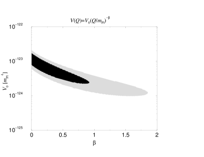
Figure 1: The 68% and 95% confidence regions for an inverse power-law model of quintessence.

II.2 Inflation

We take inflation to be driven by a scalar field $\phi$ (the inflaton) in a potential $W(\phi)$. Because of the small value of $V_{0}$, the inflaton dominates the evolution and therefore we can use the standard constraints on its parameters. The inflation model is to be chosen so as to reproduce the amplitude of perturbations needed to generate the observed structures, which requires LL

$$\frac{512\pi}{75}\,\frac{W^{3}}{m_{\mathrm{Pl}}^{6}\left|\mathrm{d}W/\mathrm{d}\phi\right|^{2}}\simeq 4\times 10^{-10}\,\mathrm{.}$$ (3)

This is to be evaluated at $\phi_{\mathrm{obs}}$, the value of the field corresponding to the epoch when the scale of the observable Universe crossed the horizon.

In this paper we will consider potentials where inflation ends by violation of the slow-roll conditions, so the slow-roll approximation

$$\varepsilon(\phi) =\frac{m_{\mathrm{Pl}}^{2}}{16\pi}\left(\frac{\mathrm{d}W/\mathrm{d}\phi}{W}\right)^{2}\ll 1$$ (4)

$$\eta(\phi) =\frac{m_{\mathrm{Pl}}^{2}}{8\pi}\frac{\mathrm{d}^{2}W/\mathrm{d}\phi^{2}}{W}\ll 1$$ (5)

gives the end of inflation and the number of $e$-foldings

$$N\simeq\frac{8\pi}{m_{\mathrm{Pl}}^{2}}\int^{\phi_{\mathrm{obs}}}_{\phi_{\mathrm{end}}}\frac{W(\phi)}{\mathrm{d}W/\mathrm{d}\phi}\,\mathrm{d}\phi\simeq 50$$ (6)

gives us $\phi_{\mathrm{obs}}$.

Fifty or so $e$-foldings is the minimum amount of inflation capable of giving our observed Universe, but crucial for the considerations of this paper is that typically one expects enormously more inflation. If one only imposes the constraint that the initial energy density be below the Planck energy, most models allow very large amounts of inflation. However the early stages of such inflation may be dominated by quantum dynamics (the so-called stochastic inflation regime SI ). The maximum value of the inflaton field we consider, $\phi_{\mathrm{max}}$, is given by the quantum-to-classical evolution transition

$$\frac{\Delta_{\mathrm{qu}}}{\Delta_{\mathrm{cl}}}=\frac{H}{2\pi}\left|\frac{H}{\dot{\phi}}\right|\lesssim 1\,,$$ (7)

where the $\Delta$ represent the typical quantum and classical evolution per Hubble time.

For simplicity we focus on a inflaton model with a power-law potential

$$W(\phi)=W_{0}\left(\frac{\phi}{m_{\mathrm{Pl}}}\right)^{\alpha}\,\mathrm{.}$$ (8)

The former constraints lead to

$$\tilde{\phi}_{\mathrm{end}} \simeq \mathrm{Max}\left[\frac{\alpha}{4\sqrt{\pi}}\,\mathrm{,}\,\sqrt{\frac{\alpha(\alpha-1)}{8\pi}}\;\right]\,\mathrm{,}$$ (9)

$$\tilde{\phi}_{\mathrm{obs}} \simeq \sqrt{\frac{50\alpha}{4\pi}+\tilde{\phi}_{\mathrm{end}}^{2}}\,\mathrm{,}$$ (10)

$$\tilde{\phi}_{\mathrm{max}} \simeq \left(\frac{3\alpha^{2}m_{\mathrm{Pl}}^{4}}{128\pi W_{0}}\right)^{1/(\alpha+2)}\,\mathrm{,}$$ (11)

$$W_{0} \simeq \frac{3\times 10^{-8}\alpha^{2}m_{\mathrm{Pl}}^{4}}{512\pi}\,\tilde{\phi}_{\mathrm{obs}}^{-(\alpha+2)}\,\mathrm{.}$$ (12)

III Quintessence field evolution during inflation

The models are now fully defined and we can study the dynamics of each field, beginning with the classical evolution.

III.1 Classical evolution

We assume that the quintessence field is completely uncoupled from everything else, including the inflaton. The equations of motion are the Euler–Lagrange equations for the inflaton and quintessence fields

$$\ddot{\phi}=-3H\dot{\phi}-\frac{\mathrm{d}W}{\mathrm{d}\phi}\quad\mathrm{;}\quad\ddot{Q}=-3H\dot{Q}-\frac{\mathrm{d}V}{\mathrm{d}Q}$$ (13)

and the Einstein equation

$$H^{2}=\frac{8\pi}{3m_{\mathrm{Pl}}^{2}}\left[\frac{1}{2}\dot{\phi}^{2}+W(\phi)+\frac{1}{2}\dot{Q}^{2}+V(Q)\right]\,\mathrm{.}$$ (14)

Because of the very small value of $V_{0}$, the evolution of the Universe is determined by the inflaton. The quintessence field may dominate if its value is very small, but, as we will see this situation would end very quickly. Therefore, using the slow-roll approximation we have the solution

$$\tilde{\phi}(N)\simeq\sqrt{\tilde{\phi}^{2}_{\mathrm{ini}}-\frac{\alpha N}{4\pi}}\,\mathrm{,}$$ (15)

where $N=\log(a/a_{\mathrm{ini}})$. The subscript “ini” always means the value at some time $t_{\mathrm{ini}}$. Knowing the dynamics of the Universe we can now study the quintessence field.

The classical behaviour of the quintessence field is rather straightforward. If the field is in a region where $\left|\mathrm{d}V/\mathrm{d}Q\right|$ is small, its classical evolution will be highly suppressed by the friction arising from the inflationary expansion and to a good approximation the field will retain its initial value. Conversely, if $\left|\mathrm{d}V/\mathrm{d}Q\right|$ is large, the field will quickly roll down until the potential becomes too flat. More precisely, using the slow-roll approximation for the quintessence field we have

$$\dot{\tilde{Q}}\simeq\frac{\beta\,V_{0}}{3H(t)m_{\mathrm{Pl}}^{2}}\,\tilde{Q}^{-\beta-1}\,\mathrm{.}$$ (16)

Assuming $H(t)$ constant (roughly correct for a few Hubble times) the solution is

$$\tilde{Q}(t)\simeq\left[\frac{\beta(\beta+2)V_{0}}{3Hm_{\mathrm{Pl}}^{2}}(t-t_{\mathrm{ini}})+\tilde{Q}_{\mathrm{ini}}^{\beta+2}\right]^{1/(\beta+2)}\,\mathrm{.}$$ (17)

We define

$$\tilde{Q}_{\mathrm{min}}=\left[\frac{\beta(\beta+2)V_{0}}{3H^{2}m_{\mathrm{Pl}}^{2}}\right]^{1/(\beta+2)}$$ (18)

and see that the evolution during a Hubble time has the following approximate description:

$$\begin{array}[]{rll}\tilde{Q}(t_{\mathrm{ini}}+H^{-1})&\simeq\tilde{Q}_{\mathrm{ini}}&\quad\mathrm{if}\quad\tilde{Q}_{\mathrm{ini}}\gg\tilde{Q}_{\mathrm{min}}\\ \tilde{Q}(t_{\mathrm{ini}}+H^{-1})&\simeq\tilde{Q}_{\mathrm{min}}&\quad\mathrm{if}\quad\tilde{Q}_{\mathrm{ini}}\ll\tilde{Q}_{\mathrm{min}}\end{array}\,\mathrm{.}$$ (19)

Therefore, after a few Hubble times the classical evolution of the quintessence field is to remain constant.

III.2 Quantum fluctuations

Although the large friction from the Hubble expansion renders the classical evolution of the quintessence field negligible, the same is not necessarily true of the quantum fluctuations. Indeed, as we shall see, the effect of these in the quintessence potential is to drive typical regions of the Universe to quite large values of the quintessence field, corresponding to low energy densities. This possibility was first mentioned in Ref. SS .

Let us now recall briefly the way we treat these fluctuations. Following Ref. LL , we choose the spatially-flat slicing and we split the quintessence field into an unperturbed part and a perturbation

$$Q(\mathbf{x},t)=Q(t)+\delta Q(\mathbf{x},t)\,\mathrm{.}$$ (20)

We quantize the perturbation and expand its Fourier components

$$\delta\hat{Q}_{\mathbf{k}}(t)=w_{k}(t)\hat{a}_{\mathbf{k}}+w^{*}_{k}(t)\hat{a}^{\dagger}_{-\mathbf{k}}\,\mathrm{,}$$ (21)

where $\hat{a}_{\mathbf{k}}$ is the annihilation operator. In the linear approximation we have to solve

$$\ddot{w}_{k}+3H\dot{w}_{k}+\left[(k/a)^{2}+m_{\mathrm{eff}}^{2}\right]w_{k}=0\,\mathrm{,}$$ (22)

where $m_{\mathrm{eff}}^{2}=\mathrm{d}^{2}V/\mathrm{d}Q^{2}$. If the field is effectively massless and $H$ is approximately constant, the power spectrum of the fluctuations is given by

$$\mathcal{P}_{k}(t)=\frac{L^{3}k^{3}}{2\pi^{2}}\left|w_{k}(t)\right|^{2}\simeq\left[1+\left(\frac{k}{aH}\right)^{2}\right]\left(\frac{H}{2\pi}\right)^{2}\,\mathrm{.}$$ (23)

This means that before horizon-crossing $\mathcal{P}_{k}(t)\propto 1/a^{2}(t)$ and afterwards it becomes constant. Using

$$\langle\delta\hat{Q}^{2}(\mathbf{x},t)\rangle=\int^{\infty}_{0}\mathcal{P}_{k}(t)\frac{\mathrm{d}k}{k}\,\mathrm{,}$$ (24)

and the fact that the fluctuations become classical after they cross the horizon, we find that the quintessence field receives quantum kicks whose size is estimated as $H/2\pi$ per Hubble time.

The effect of these quantum fluctuations can be studied using the Fokker–Planck formalism SI2 , which allows one to follow the probability distribution $f(Q,t)$ of the quintessence field during inflation. A simple derivation is as follows. We take discrete steps $\Delta t=H^{-1}\varepsilon$ during which there are a random jump of magnitude $\Delta Q_{\mathrm{qu}}=\sqrt{\Delta t/H^{-1}}H/2\pi=\sqrt{\Delta\varepsilon}H/2\pi$ due to quantum fluctuations and a classical step $\Delta Q_{\mathrm{cl}}=\dot{Q}\Delta t=-\varepsilon V^{\prime}/3H^{2}$, where the prime denotes a derivative with respect to $Q$. During this time an interval $\mathrm{d}Q$ shrinks by a factor $1+\varepsilon V^{\prime\prime}/3H^{2}$. We find the following equation:

$$\begin{split}f(Q,t+\Delta t)\mathrm{d}Q=&\,\frac{1}{2}\Big{[}f(Q-\Delta Q_{\mathrm{cl}}+\Delta Q_{\mathrm{qu}},t)\\ &+f(Q-\Delta Q_{\mathrm{cl}}-\Delta Q_{\mathrm{qu}},t)\Big{]}\\ &\times(1+\varepsilon V^{\prime\prime}/3H^{2})\,\mathrm{d}Q\,\mathrm{.}\end{split}$$ (25)

Subtracting $f(Q,t)\mathrm{d}Q$, dividing by $\varepsilon$ and taking the limit $\varepsilon\to 0$ leads to

$$\begin{split}\frac{\partial f(Q,t)}{\partial t}=&\,\frac{H^{3}(t)}{8\pi^{2}}\,\frac{\partial^{2}f(Q,t)}{\partial Q^{2}}\\ &+\frac{1}{3H(t)}\frac{\partial}{\partial Q}\left(\frac{\partial V(Q)}{\partial Q}\,f(Q,t)\right)\,\mathrm{.}\end{split}$$ (26)

On the right-hand side, the first term produces diffusion and the second one produces a drift. Note that unlike the usual stochastic inflation situation, here $H(t)$ is determined externally by the inflaton field evolution, and the fluctuations in $Q$ do not back-react on the expansion rate.

To be complete we need the boundary condition

$$\lim_{Q\to 0}\left[\frac{H^{3}(t)}{8\pi^{2}}\frac{\partial f(Q,t)}{\partial Q}+\frac{\partial V(Q)/\partial Q}{3H(t)}f(Q,t)\right]=0\,\mathrm{,}$$ (27)

the requirement that $f(Q,t)\geq 0$, and normalization $\int_{0}^{\infty}f(Q,t)\mathrm{d}Q=1$ which implies $\lim_{Q\to\infty}f(Q,t)=0$.

From now on we focus on the inverse power-law potential for the quintessence. First of all, one may wonder whether the massless condition we used for the typical quantum jump is justified. Indeed, for values smaller than $Q_{\mathrm{lim}}$, where

$$\tilde{Q}_{\mathrm{lim}}=\left[\frac{\beta(\beta+1)V_{0}}{H^{2}m_{\mathrm{Pl}}^{2}}\right]^{1/(\beta+2)}\,\mathrm{,}$$ (28)

the quintessence field has an effective mass $m_{\mathrm{eff}}$ which is no longer negligible compared to the Hubble rate. For all wavelengths $a/k$ bigger than $1/m_{\mathrm{eff}}$, Eq. (22) implies

$$w_{k}(t)\propto a^{-3/2}(t)$$ (29)

and therefore the power spectrum of $P_{k}(t)$ decreases as $1/a^{3}(t)$ leading to a smaller value of the quantum jump after horizon-crossing. Nevertheless, because the typical quantum jump $H/2\pi$ (typically $10^{-5}m_{\mathrm{Pl}}$) is dramatically bigger than $Q_{\mathrm{lim}}$ (with $\beta=1$, typically $10^{-39}m_{\mathrm{Pl}}$), the massless condition is broken only during very short periods of time (much less than a Hubble time) and so the massless approximation is an excellent one.

The Fokker–Planck equation becomes

$$\begin{split}\frac{\partial f(Q,t)}{\partial t}=&\,\frac{H^{3}(t)}{8\pi^{2}}\,\frac{\partial^{2}f(Q,t)}{\partial Q^{2}}\\ &-\frac{\partial}{\partial Q}\left(\frac{\beta V_{0}m_{\mathrm{Pl}}^{\beta}}{3H(t)}Q^{-\beta-1}\,f(Q,t)\right)\,\mathrm{.}\end{split}$$ (30)

For $Q>Q_{\mathrm{min}}$ we can drop the terms coming from the classical evolution since we have seen it is negligible. For $Q<Q_{\mathrm{min}}$ the effect of the potential becomes important and it acts as a wall preventing the quantum fluctuations driving the quintessence field to the origin. Therefore, to a good approximation we have to solve

$$\frac{\partial f(Q,t)}{\partial t}=\frac{H^{3}(t)}{8\pi^{2}}\,\frac{\partial^{2}f(Q,t)}{\partial Q^{2}}\,\mathrm{,}$$ (31)

with the boundary condition $\mathrm{d}f(Q\approx 0,t)/\mathrm{d}Q=0$ (no flux through the origin) and maintaining $f(Q,t)\geq 0$ and $\int_{0}^{\infty}f(Q,t)\mathrm{d}Q=1$. This is equivalent to a random walk with a wall. Starting with a (half) Gaussian distribution centred on $Q=0$ and with variance $\sigma^{2}(t)$, and assuming $H(t)$ is constant during $\Delta t$, we have

$$\sigma^{2}(t_{\mathrm{ini}}+\Delta t)=\sigma_{\mathrm{ini}}^{2}+\frac{H^{3}}{4\pi^{2}}\,\Delta t\,\mathrm{.}$$ (32)

More precisely, the equation to solve is

$$\frac{\mathrm{d}\sigma^{2}}{\mathrm{d}t}=\frac{H^{3}(t)}{4\pi^{2}}\,\mathrm{,}$$ (33)

which has solution

$$\sigma^{2}(\tilde{\phi})\simeq\sigma^{2}_{\mathrm{ini}}+\frac{16W_{0}}{3\alpha(\alpha+2)m_{\mathrm{Pl}}^{2}}\left(\tilde{\phi}_{\mathrm{ini}}^{\alpha+2}-\tilde{\phi}^{\alpha+2}\right)\,\mathrm{.}$$ (34)

After enough time the evolution is roughly independent of the initial condition $\sigma_{\mathrm{ini}}$ and we can set it to zero.

Figure 2: Probability distributions for the mean quintessence value at the end of inflation for different initial values $\phi_{\mathrm{ini}}$, in the particular case of $\alpha=2$. We have also plotted the probability distribution obtained by averaging over $\phi_{\mathrm{ini}}$.

We can now ask what one expects the mean value of the quintessence field to be in our region of the Universe. Because we are presently interested only in the mean value, we should only consider perturbations on scales larger than our present horizon, which are generated between the initial inflaton value $\phi_{\mathrm{ini}}$ and $\phi_{\mathrm{obs}}$. Because of the presence of the wall, the net effect of the quantum fluctuations is to diffuse the quintessence field to larger values. The extent of this diffusion depends on how much inflation occurs before the last fifty $e$-foldings; if more inflation occurs then there are more ‘steps’ in the diffusion and also the early steps are larger. We have also computed the distribution obtained by averaging over all possible initial inflaton values between $\phi_{\mathrm{obs}}$ and $\phi_{\mathrm{max}}$ assuming a flat probability.

Actually we are more interested in the probability distribution $f_{q}$ of $q=\log_{10}(Q/m_{\mathrm{Pl}})$. We have $f_{q}(q,t)=f(Q(q),t)\mathrm{d}Q/\mathrm{d}q$ which has a peak at $q_{\mathrm{peak}}=\log_{10}(\sigma(t)/m_{\mathrm{Pl}})$. In Fig. 2 we show some distributions $f_{q}(q,t_{\mathrm{obs}})$ in the particular case of $\alpha=2$; we show the probability distributions for two possible initial conditions for the inflaton, and then the probability distribution averaged over a uniform initial distribution for $\phi_{\mathrm{ini}}$ between $\phi_{\mathrm{obs}}$ and $\phi_{\mathrm{max}}$. Fig. 3 shows the position of the peak in the distributions as a function of $\alpha$; as we can see, the result is roughly independent of $\alpha$, and as expected the more inflation there is the further the distribution diffuses to large $Q$.

Figure 3: The position of the peak of the probability distributions of $Q$, as in Fig. 2, plotted as a function of $\alpha$.

We wish to know the quintessence value after inflation to assess when the solution begins tracking. In the slow-roll approximation, the solution for the tracker is

$$\tilde{Q}(a)\simeq\left(\frac{\beta(\beta+2)V_{0}}{24\pi\rho_{\mathrm{f}0}(1+w_{\mathrm{f}})}\right)^{1/(\beta+2)}\left(\frac{a}{a_{0}}\right)^{3(1+w_{\mathrm{f}})/(\beta+2)}\,\mathrm{,}$$ (35)

where $\rho_{\mathrm{f}0}$ is the present value of the energy density and $w_{\mathrm{f}}$ the pressure–density ratio of the dominant fluid (either radiation or non-relativistic matter). Some examples of trackers are plotted in Fig. 4. After inflation the quintessence field remains constant as long as its energy density is lower than the tracker’s. We can therefore find the probability distribution $f_{z}$ for $\log_{10}(z_{\mathrm{tr}}+1)$, where $z_{\mathrm{tr}}$ is the redshift at which the quintessence reaches the tracking behaviour, by comparing the value of $Q$ at the end of inflation with the tracking solution. Using Fig. 3 and Fig. 4 we can estimate at which redshift the tracker is reached for some values of $\alpha$ and $\beta$. We notice that the smaller $\beta$ is, the later the tracker is reached for a given initial value of $Q$. In Fig. 5 we show some examples of distributions for the redshift at which tracking begins. The discontinuity in the distribution comes from the fact that at about radiation–matter equality there is a transition between two trackers.

Figure 4: Some examples of trackers for different values of $\beta$.

The striking feature of this figure is how low the expected redshift of tracking is. While some previous papers have advocated equipartition of the quintessence energy density as an initial condition equip , leading to prompt tracking, we find that tracking is postponed until the late stages, and in particular well after nucleosynthesis. Indeed, the bulk of the probability is not only after nucleosynthesis but after decoupling too; however there is only a small probability that tracking has not begun by the present, which would not lead to acceptable quintessence.

Figure 5: Probability distributions for the redshift at which the quintessence field reaches the tracker, for $\alpha=2$ and $\beta=1$. The distributions are shown for two different initial values $\phi_{\mathrm{ini}}$, and averaged over $\phi_{\mathrm{ini}}$. The discontinuities arise across matter–radiation equality.

Finally we must say that our results are valid for small initial values of the quintessence field before inflation (in fact formally zero). If this were not the case, the probability distribution for the mean value of the quintessence field at the end of inflation will broaden to larger values and the tracker will be reached even later or not at all.

IV Conclusions

We have analyzed the quantum dynamics of the quintessence field during a period of early Universe inflation. Due to quantum fluctuations, even if the initial value of $Q$ in a certain region of the Universe is small, it is rapidly diffused to large field values and hence low energy density. We have found that typically tracking behaviour begins only at quite a late stage of evolution, well after nucleosynthesis and quite likely after decoupling too.

Although we have discussed specific models of both inflation and quintessence, we expect our results to be quite general; as far as inflation is concerned we need only the assumption that there are significantly more than fifty $e$-foldings in total and a standard value of $H$ during inflation, while for other models of quintessence where the potential diverges at the origin the result should also be the same as the precise form of the potential is dynamically irrelevant. In particular, while we have only considered models where the tracking density during nucleosynthesis is negligible, these considerations may reinstate models whose tracking density would be unacceptable during nucleosynthesis.

- (1) C. Wetterich, Nucl. Phys. B302, 668 (1988).
- (2) B. Ratra and P. J. E. Peebles, Phys. Rev. D37, 3406 (1988).
- (3) E. J. Copeland, A. R. Liddle, and D. Wands, Ann. N. Y. Acad. Sci. 688, 647 (1993); P. G. Ferreira and M. Joyce, Phys. Rev. Lett. 79, 4740 (1997), astro-ph/9707286, Phys. Rev D 58, 023503 (1998), astro-ph/9711102; M. Yahiro, G. J. Mathews, K. Ichiki, T. Kajino, and M. Orito, Phys. Rev. D65, 063502 (2002), astro-ph/0106349.
- (4) E. J. Copeland, A. R. Liddle, and D. Wands, Phys. Rev. D57, 4686 (1998), gr-qc/9711068; A. R. Liddle and R. J. Scherrer, Phys. Rev. D59, 023509 (1999), astro-ph/9809272.
- (5) I. Zlatev, L. Wang, and P. J. Steinhardt, Phys. Rev. Lett. 82, 896 (1999), astro-ph/9807002; P. J. Steinhardt, L. Wang, and I. Zlatev, Phys. Rev. D59, 123504 (1999), astro-ph/9812313.
- (6) R. Bean, S. H. Hansen and A. Melchiorri, Phys. Rev. D64, 103508 (2001), astro-ph/0104162.
- (7) P. J. E. Peebles and A. Vilenkin, Phys. Rev. D59, 063505 (1999), astro-ph/9810509; E. J. Copeland, A. R. Liddle, and J. E. Lidsey, Phys. Rev. D64, 023509 (2001), astro-ph/0006421; G. Huey and J. E. Lidsey, Phys. Lett. B514, 217 (2001), astro-ph/0104006.
- (8) P. Brax, J. Martin, and A. Riazuelo, Phys. Rev. D62, 103505 (2000), astro-ph/0005428; M. Doran, M. Lilley, and C. Wetterich, Phys. Lett. B528, 175 (2002), astro-ph/0105457; P. S. Corasaniti and E. J. Copeland, Phys. Rev. D65, 043004 (2002), astro-ph/0107378; C. Baccigalupi, A. Balbi, S. Matarrese, F. Perrotta, and N. Vittorio, Phys. Rev. D65, 063520 (2002), astro-ph/0109097
- (9) R. Bean, S. H. Hansen, and A. Melchiorri, astro-ph/0201127.
- (10) W. L. Freedman et al., Astrophys. J. 553, 47 (2001), astro-ph/0012376.
- (11) A. R. Liddle and D. H. Lyth, Cosmological Inflation and Large-Scale Structure, Cambridge University Press, Cambridge, 2000.
- (12) A. Vilenkin, Phys. Rev. D27, 2848 (1983); A. D. Linde, Phys. Lett. B175, 395 (1986).
- (13) V. Sahni and A. Starobinsky, Int. J. Mod. Phys. D9, 373 (2000), astro-ph/9904398.
- (14) A. D. Linde and A. Mezhlumian, Phys. Lett. B307, 25 (1993), gr-qc/9304015; A. D. Linde, D. Linde, and A. Mezhlumian, Phys. Rev. D49, 1783 (1994), gr-qc/9306035.