High-Resolution X-ray imaging and spectroscopy of SNR N 103B

The X-ray emission from the young supernova remnant (SNR) SNR N 103B is measured and analysed using the high-resolution cameras and spectrometers on board XMM-Newton and Chandra. The spectrum from the entire remnant is reproduced very well with three plasma components of $kT_{\rm e}$ = 0.55, 0.65, and 3.5 keV, corresponding roughly to line emission by the O-K, Fe-L, and Fe-K species, respectively. Narrow band images reveal different morphologies for each component. The $kT_{\rm e}$ = 0.65 keV component, which dominates the emission measure (4.5$\times$10⁶⁵m^-3), is in ionisation equilibrium. This provides a lower limit of 3000 yrs to the age of the remnant, which is considerably older than the previously assumed age of the remnant (1500 yrs). Based on the measured energy of the Fe-K feature at 6.5 keV, the hot (3.5 keV) component is found to be recently shocked ($\sim$200 yrs) and still ionising. The high elemental abundances of O and Ne and the low abundance of Fe could imply that SNR N 103B originated from a type II supernova (SN) rather than a type Ia SN as previously thought.

1 Introduction

The young supernova remnant (SNR) N 103B (also known as SNR 0509-69) is the fourth brightest X-ray remnant in the Large Magellanic Cloud (LMC). It was first identified as a supernova remnant by Mathewson and Clarke (mathewson (1983)) based on the non-thermal nature of its radio spectrum and the relative emission-line strengths of S ii and H$\alpha$. Due to its small size (3 pc), Hughes et al. (hughes (1995)) estimated the age of SNR N 103B to be about 1500 yrs. Recent Chandra data (Lewis et al. lewisa (2001)) show that the remnant is much brighter on the western limb than towards the East, this is most likely because of density contrasts between East and West. The radio and X-ray brightness variations are correlated on large scales, but do not overlap on finer spatial scales (Hughes hughes01 (2001)). In the analysis of the moderate resolution CCD ASCA spectrum of SNR N 103B, Hughes et al. (hughes (1995)) found strong emission lines from Si, S, Ar, Ca, and Fe, while no emission from O, Ne, or Mg was required in order to fit the ASCA spectrum. Hughes et al. (hughes (1995)) thus concluded that SNR N 103B is the result of a Type Ia supernova. However, its proximity to the star cluster NGC 1850 and the H II region DEM 84 suggest that SNR N 103B has an early-type progenitor (Chu & Kennicutt chu (1988)), providing contradictory evidence for the nature of the progenitor.

In this work, we present the X-ray spectra of SNR N 103B measured by the XMM-Newton suite of scientific instruments, i.e. the Reflection Grating Spectrometers (RGS) and the European Photon Imaging Cameras (EPIC). Particularly, we exploit the high dispersion of the RGS and its unique capability to resolve line emission from extended sources to investigate the nature of the hot plasma in SNR N 103B in unprecedented detail and to shed new light on its progenitor. The large effective area of the EPIC cameras at high energies also allows us to study the important Fe-K emission. All these are complemented by the sharp images produced with the high angular resolution of the Advanced CCD Imaging Spectrometer (ACIS) on board Chandra, which reveal the temperature dependent morphology of SNR N 103B.

2 Observation and Data Reduction

SNR N 103B was observed by XMM-Newton on 7 August 2000. The effective exposure times and filters used on the different instruments are summarised in table 1. The RGS data were processed using custom software that is identical in function to the RGS branch of the Science Analysis System (SAS), which was described briefly by Rasmussen et al. (andy (2001)). It includes pixel by pixel CCD event offset subtraction using median diagnostic frames, position dependent CTI correction, and correction of dispersion angles imparted by aspect drift.

Table 1: XMM-Newton observation data of SNR N 103B

Instrument Filter Exposure Time (ks) MOS 1 Thick 8.0 MOS 1 Medium 8.0 MOS 2 Medium 23.5 PN Medium 9.5 RGS 1 32.3 RGS 2 32.4

We chose this analysis path since our response matrix generator features support for extended targets, and details in the angular distribution of SNR N 103B were included in the response matrices. A single, broad-band archival ROSAT HRI image was used, along with mean spacecraft aspect and our spectral extraction angular width, to predict the monochromatic response in the readout channel space. This modelling approach breaks down as soon as the target’s morphology depends strongly on wavelength. However, it still permits accurate measurement of total line intensities and significant velocity distributions that distort line profiles in the RGS. In the case of SNR N 103B, wavelength dependent variations in morphology appear on scales comparable to the XMM-Newton mirror point spread function (PSF), and our modelling approach remains reasonable for the purposes described. However, we do still expect to observe small ($\sim$20 mÅ) wavelength shifts for some lines due to variations in the remnant’s morphology.

The raw EPIC data were initially processed with the XMM-Newton SAS. This involved the subtraction of hot, dead, or flickering pixels, as well as removal of events due to electronic noise. The spectrum was extracted from a circular region with a radius of 1.5′. Background subtraction for EPIC was done using an exposure of the Lockman hole, with similar data selections and the same extraction region as for the SNR, scaling according to the exposure time. Periods of high particle background were rejected based upon the $10-12$ keV count rate for the entire field of view.

In order to support our spectral analysis of the entire remnant with spatially resolved information on the morphology, we also used archival Chandra data of SNR N 103B, which was observed with the back-illuminated ACIS-S3 chip on 4 December 1999 (see also Lewis et al. lewisa (2001)). The cleaned event list was taken from the public Chandra archive. Narrow band images were extracted with energy selections made according to the nominal energy column, which provides a good energy estimate of each recorded photon.

3 Data Analysis

3.1 XMM-Newton Spectra

The RGS spectrum of SNR N 103B is shown in figure 1. The spectrum is dominated by emission lines from highly ionised species of O, Ne, Mg, Si, & Fe. No emission longward of 23 Å is detected. This can probably be attributed to line-of-sight absorption towards the LMC rather than to the absence of N and C species, which could have been readily detected by the RGS. An important point to note is that we clearly detect O, Ne, and Mg lines. The O vii and O viii lines are particularly strong. These features were not detected in the CCD spectrum of SNR N 103B obtained with ASCA (Hughes et al hughes (1995)), nor in a more recent CCD measurement with Chandra ACIS (Lewis et al. lewisa (2001)). In order to observe shorter wavelengths than provided by the RGS  we also employ the EPIC-MOS CCD spectrum, which is presented in figure 2. Emission lines from He-like S, Ar, Ca, as well as an Fe-K blend at 6.5 keV are clearly observed.

Figure 1: The fluxed RGS of SNR N 103B spectrum. The most prominent lines are labeled.

Figure 2: The EPIC-MOS of SNR N 103B spectrum. The solid line is the best-fit 3 component NEI model. The most prominent line blends are labeled.

The spectral analysis was performed using the SRON SPEX package (Kaastra et al. kaastra (1996)), which contains the MEKAL atomic database (Mewe et al. mewe (1995)) for thermal emission. Both Coronal Ionisation Equilibrium (CIE) and non-equilibrium ionisation (NEI) models are available in SPEX. Our model for the X-ray emission of SNR N 103B consists of several plasma components. For each component, we fit for the volume emission measure ($n_{\rm e}n_{\rm H}V$), the electron temperature ($T_{\rm e}$), the elemental abundances, the redshift of the source, and the Hydrogenic column density $N_{\rm H}$ of neutral absorbing gas along the line of sight. In NEI models, the ionisation age ($n_{\rm e}t$) (Kaastra & Jansen net (1993)) is also a free parameter. Here, $n_{\rm e}$ is the electron density, $n_{\rm H}$ is the hydrogen density, $V$ is the volume of emitting gas and $t$ is the time since the material has been shocked and heated to its current temperature. A distance of 51 kpc to the LMC is assumed (Feast et al. feast (2002)).

In the following, we describe the procedure used to fit the total spectrum emitted by the whole remnant. The entire procedure was carried out for both CIE and NEI scenarios for comparison. We fitted the RGS spectrum first, since it has the most details and therefore is most constraining. Two plasma components are sufficient for obtaining a good fit to the RGS spectrum. Assuming that most of the X-ray emission is due to gas with more or less similar composition, we coupled the elemental abundances in the two components. This also minimises the number of free variables in our fit, which makes it more robust.

It is clear from the EPIC spectrum that SNR N 103B also has a hot component that is hard for the RGS to distinguish. In order to model this component, we fit the CCD spectrum of EPIC with three plasma components. We coupled the elemental abundances of O, Ne, Mg, Si, S, Ar & Ca of the third component to those of the two cooler components. The Fe abundance, however, is left free since we cannot fit the Fe-L and Fe-K with the same abundance value. The electron temperature, ionisation age and abundances of the two cooler components are fixed at the values obtained by the RGS fit. We note, however, that the hot component is not very sensitive to the other two components even when all three components are fitted simultaneously. In principle, the EPIC spectra could be fitted well with only two plasma components, i.e., without the relatively cold one. This explains why previous CCD observations did not detect the low-temperature component, which is dominated by O emission. It is only because of the spectral resolution of the RGS and its sensitivity to soft X-rays ($>$ 20 Å) that we are able to resolve the O vii emission and hence need a cool or under-ionised component in the model. Finally, for consistency and in order to obtain the ultimate fit, we return to the RGS spectrum and refit it with three components. The hot component, which is constrained by the EPIC, but hardly produces line emission in the RGS spectrum is fixed at its EPIC values. The final parameters obtained for the three components are presented in Table 2 for both the CIE and NEI cases. We obtain a best-fit column density of $N_{\rm H}=(2.5{\pm}0.7){\times}10^{25}$ m^-2. We also obtain a redshift of 340$\pm$70 km s^-1, which is consistent with the radial velocity of the LMC ($v_{\hbox{LMC}}=278$ km s^-1). The significance of NEI as well as the elemental abundances resulting from the fits are discussed below in §4.

Table 2: Spectral fitting results. Components 1 & 2 reflect the RGS results, since the RGS is more robust at constraining the parameters in this spectral range. Component 3 is required to account for the Fe-K emission in the EPIC Data.

Parameter Covered by CIE NEI Component 1: $n_{\rm e}n_{\rm H}V$ (10⁶⁴m^-3) 6.2$\pm$0.8 2.6$\pm$0.1 $kT_{\rm e}$ (keV) RGS 0.21$\pm$0.05 0.55${}^{+0.05}_{-0.32}$ $n_{\rm e}t$ (10¹⁶ m^-3s) 2.3${}^{+10}_{-0.3}$ redshift (kms^-1) 340$\pm$70 340$\pm$70 Component 2: $n_{\rm e}n_{\rm H}V$ (10⁶⁴m^-3) RGS 65.1$\pm$1.1 65.2$\pm$1.2 $kT_{\rm e}$ (keV) + 0.65$\pm$0.05 0.65$\pm$0.05 $n_{\rm e}$t (10¹⁶ m^-3s) EPIC $>$250 redshift (kms^-1) 340$\pm$70 340$\pm$70 Component 3: $n_{\rm e}n_{\rm H}V$ (10⁶⁴m^-3) 4.1$\pm$0.4 4.1$\pm$0.5 $kT_{\rm e}$ (keV) EPIC 3.5$\pm$0.5 3.5$\pm$0.5 $n_{\rm e}t$ (10¹⁶ m^-3s) 5.3$\pm$0.8 redshift (kms^-1) 4100$\pm$300 340$\pm$70 ${\chi}^{2}$/d.o.f 1810/902 1790/899

The best-fit spectral NEI model for SNR N 103B is compared with the EPIC-MOS and RGS spectra in figures 2 and 3, respectively. The CIE model fits the data nearly as well. The overall fit to the data is very good. For the most part, the fit residuals are consistent within instrumental calibration uncertainties. However, some small discrepancies remain in the fit. The most prominent discrepancy is the missing flux in the model for the 2p–3s lines of Fe xvii at $\sim$17 Å. This is a well known problem and has been observed in many coronal sources and in the laboratory. Therefore, it probably has nothing to do with NEI effects, although in principle NEI could enhance the 17 Å lines with respect to the 15 Å lines by means of inner-shell ionisation of Fe XVI. Doron & Behar (doron (2002)) suggest a model that could rectify the standard collisional-excitation line powers in MEKAL and in APEC (Smith et al. apec (2001)). They show that including resonant excitation as well as recombination and ionisation processes (in CIE) from neighbouring ions in the models considerably enhances the 2p-3s lines and consequently produces the observed line ratios. Most of the other discrepancies in figure 3 have local asymmetrical profiles, which are a result of a combination of the following: (i) difference between the broadband spatial profile used in the response and the actual spatial profiles of individual emission lines, (ii) slight errors in model or data wavelengths, (iii) slight errors in the line spread function which does not account for the real asymmetrical profile of the RGS line shapes. The first of these sources of errors (i.e. the spatial profile used) should, however, dominate. There is also a slight overestimation of the continuum (in the range 18–23 Å) in the models, which is most likely due to uncertainties in the background subtraction. These inconsistencies between data and models are small and do not affect the conclusions drawn in this paper.

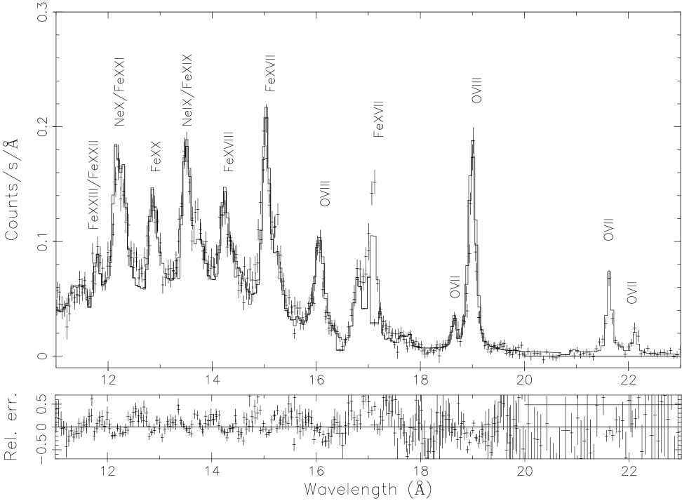
Figure 3: The RGS spectrum in the range 11-23 Å. The solid line represents a best-fit 2 component NEI model ($kT_{\rm e}=$0.65 & 0.55 keV) plus an underlying $kT_{\rm e}=$3.5 keV component as obtained from the EPIC-MOS fits. The overall fit to the data is good. The missing flux in the model for the 2p–3s lines of Fe xvii at $\sim$17 Å is a known problem which is due missing transitions in the plasma code (see text).

3.2 Chandra Images

In figure 4 we present three narrow-band images obtained with the ACIS camera. The images are produced in the energy ranges of 0.5–0.7, 0.7–1.0, and 3.0–6.8 keV. The first image (0.5–0.7 keV) is essentially an image of O-K emission (O VII and O VIII). The second image (0.7–1.0 keV) represents predominantly Fe-L emission and the third image (3–6.8 keV) reflects the morphology of Ar-K, Ca-K, and Fe-K lines, as well as some continuum. We have also separated this high-energy band into its various sub-component images (Ar, Ca, and Fe). However, within the statistics available for these images, all their morphologies appear to be fairly similar. The three images in figure 4 correspond roughly to the three plasma components described in Table 1, in respective order. For short, we will henceforth refer to these three energy bands (and their respective plasma components) simply as the O-K, Fe-L, and Fe-K bands (components).

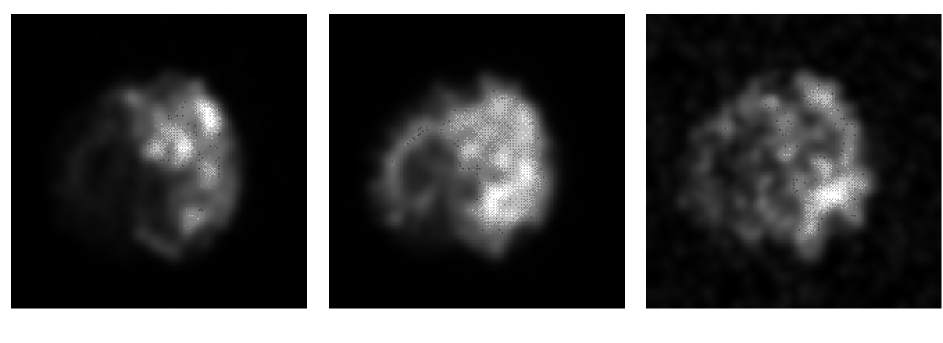
Figure 4: Chandra images for the approximate energy range 0.5–0.7 keV (left), 0.7–1.0 keV (centre) and 3–6.8 keV (right). These three energy bands are dominated by emission from O vii & ionOviii (0.5–0.7 keV), Fe-L (0.7–1.0 keV)and Ar, Ca, Fe-K and continuum (3–6.8 keV).

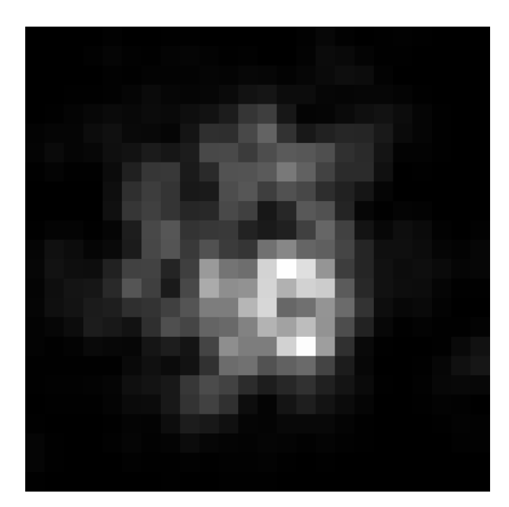
Figure 5: The deconvolved XMM-Newton Fe-K image. The Fe-K image reveals a bright emission spot towards the southwestern rim of the remnant.

All three images in figure 4 show the same asymmetry, where the western hemisphere is much brighter than the eastern hemisphere. Aside from that, they are quite different in morphology. The O-K emission is concentrated in the northwest, while the Fe-L emission is more evenly distributed along the western rim of the remnant. The Fe-K image reveals a bright emission spot located at the southwestern rim. We also created a continuum subtracted, deconvolved, XMM-Newton Fe-K (i.e 6.3–6.8 keV) image (see van der Heyden et al. kurt (2002) for details). The XMM-Newton Fe-K image (figure 5) also shows a bright emission spot located at the southwestern rim, but extends further inward than seen in the Chandra 3–6.8 keV image. However, while the statistics are of the XMM-Newton image is superior the ability to extract more information on the morphology of the remnant is hampered by the lower spatial resolution of the XMM cameras.

A more subtle difference between the emission in the three different bands is their radial distribution. In order to obtain a further insight into the radial distribution, we plotted the normalised radial profiles in counts per second in the three bands. These profiles in counts per pixel are presented in figure 6. Each profile is normalised separately to the average count rate measured in its energy range within a radius of 17.5″. Despite the differences in azimuthal distribution, it can be seen that the (normalised) brightness of all three components is surprisingly similar; peaking at approximately 4″, 7″, and 10″. The Fe-L component (dashed curve) lies slightly (0.5″), but consistently inside the other two components. Normalising the radial profiles to their peak values does not alter this conclusion.

Figure 6: Normalised radial emission profiles for three separate photon-energy bands: 0.5–0.7 (dashed curve), 0.7–1.0 (solid curve), and 3–6.8 keV (dotted curve).

4 Discussion

4.1 Ionisation equilibrium

As demonstrated by the fitting results in Table 2, the RGS spectrum can be described similarly well by either a set of NEI or CIE plasma components, giving ${\chi}^{2}$/d.o.f. of 1790/902 and 1810/899, respectively, for the two methods. Moreover, both models yield very similar spectra. In terms of emission measure, the X-ray spectrum of SNR N 103B is dominated by the Fe-L component (2). This emission component is represented by an electron temperature of $kT_{\rm e}=0.65$ keV in both models. The NEI model yields a very high ionisation age ($n_{\rm e}t\geq 2.5\times 10^{18}$ m^-3s) for this component, which is sufficiently high for the plasma to be in or very close to equilibrium (see Mewe mewe2 (2002)).

For the weaker and cooler O-K component (1), which produces the O VII and most of the O VIII emission, the two methods actually give very different temperature and emission measure values. In CIE conditions, these O ions form at a relatively low temperature (0.2 keV in the best-fit CIE model). In the case of NEI, on the other hand, this component is much hotter (0.55 keV), but still ionising (n_et$\sim$2.3$\times$10¹⁶ m^-3 s). Both models reproduce the observed line intensities equally well. Note that the very large errors associated with the temperature (-0.32 keV) and ionisation time (+1e17 m³s) in the NEI model are due to the fact that the fitting routing finds another minimum at $\sim$0.2 keV in the case of equilibrium ionisation, as expected. A comparison of the best-fit models for the O VII lines in both approaches is shown in figure 7. The differences between the NEI and CIE fits can be seen to be small, which implies that the data do not decidedly favour one scenario over the other. This CIE/NEI ambiguity in the O VII lines was recognised before in the analysis of the RGS spectrum of the LMC remnant N132D (Behar et al. ehud (2001)). It should be noted that the ambiguity of NEI/CIE in the O-K component (1) does not affect the fits for the other components at all, i.e., we get the same parameters for components 2 and 3, regardless of whether component 1 is in NEI or CIE.

Figure 7: Comparison of NEI and CIE fits to the O vii Helium-like triplet. The crosses are the RGS data points in the 21.3-22.3 Å range. The solid line is the $kT_{\rm e}=0.55$ keV NEI model while the dashed line is the $kT_{\rm e}=0.2$ keV CIE model. Both models provide fits of similar quality, making it difficult to distinguish between the models.

The most outstanding evidence for NEI conditions emerges from the hot Fe-K component (3), which is responsible for the Fe-K feature measured at 6.5 keV, as displayed in figure 8. An attempt to model this feature as a CIE He-like Fe line (restframe energy 6.7 keV) requires that it be redshifted by $\sim 4100$ km s^-1 with respect to the LMC systemic velocity. Such a large redshift is not observed for the Ar-K nor the Ca-K lines, which arise from the same component as Fe-K and overlap spatially. This makes the large redshift interpretation unlikely. An alternative and more plausible explanation for the spectral position of the Fe-K complex would be a relatively low ionisation age of $n_{\rm e}t{\sim}5.3{\times}10^{16}$ m^-3s for the hot component, as obtained by our NEI fit (see Table 2) without any additional redshift. This NEI component predicts a distribution of Fe charge states that peaks between Fe xix and Fe xxiv. This component also contributes most of the flux in the Ar and Ca lines and provides good fits to these lines.

Figure 8: The EPIC-PN spectrum in the range 5.5-7.5 keV, showing the Fe-K plot. The solid line is a $kT_{\rm e}=3.5$ keV model fit. The location of the line centroid ($\sim$6.5 keV) indicates that the gas is not in ionisation equilibrium.

4.2 Density, age, and dynamics

The electron density can be calculated from the emission measure ($n_{\rm e}n_{\rm H}V$) if we know the volume of the emitting region. For simplicity, we generally assume the emitting volume to be a thick spherical shell. Based on the emission maps provided in figure 4 and on the radial profiles shown in figure 6, the shell is taken to have a radius of $R$ = 15″ and to be $\Delta R$ = R/10 = 1.5″ thick (Lozinskaya lozinskaya (1992)). At a distance of 51 kpc, it gives a volume of $V=1.7{\times}10^{51}{\times}f$ m³, where $f$ is a volume filling factor. This is a very crude estimate of the volume, but it is sufficient for our order-of-magnitude estimates that follow.

For the dominant Fe-L component (2), which seems to cover most of the western hemisphere (see figure 4), we assume a half filled shell or $f$ = 0.5, which gives an electron density of $n_{\rm e}\sim 25{\times}10^{6}$ m^-3. Using this density and the ionisation age ($n_{\rm e}t$) from Table 2, we get for the time since the Fe-L gas was shocked: $t\geq$ 3000 yrs. This time is considerably longer than the previously assumed age of the remnant (1500 yrs), however, the age derived from the ionisation time assumes constant density and does not take into account the expansion of the shell.

Since the Fe-K component is concentrated in the southwestern region of the remnant (see figure 4), we estimate the filling factor to be $f$ = 0.25. This gives an electron density of $\sim 8{\times}10^{6}$ m^-3, which in turn yields an age of $\sim$200 yrs. This is a relatively short time and is particularly in contrast with the derived age of the Fe-L component. For component 1, the bulk of the O-K emission is located towards the NW rim of the remnant. We again assume a filling factor of $f=0.25$. This yields electron densities of 7.$1{\times}10^{6}$ and $10.6{\times}10^{6}$ m^-3 for the NEI and CIE models, respectively. If the NEI model is preferred, its ionisation time would then also imply a time of about 100 yrs since shock heating. Note the comparable ages of the O-K and Fe-K components. On the other hand, the different locations (figure 4) and vastly different temperatures of these two components strongly suggest that they may not be dynamically connected.

Indeed, each of the three spectral components can be identified spatially. As discussed earlier and as seen in figure 4, the various spectral components show substantial variation in morphology. Given our spectral analysis and due to the fact that roughly comparable densities are obtained for all of these components, it is most likely that these variations are due to gradients in temperature and ionisation ages. The different locations and temperatures of the three components suggest that they are probably unrelated dynamically. Despite these morphological differences the azimuthal average emission profiles show a remarkable similarity. Even more surprising is that, compared to the Fe L component, the coolest (O vii/O viii) and the hottest component peak at a larger radius, extend further out, and seem to be the most recently shocked components. This would suggest that these components are associated with material recently shocked by the blast wave, whereas the Fe L component may be plasma heated by the reverse shock. However, the overabundance of Ar, Ca and Fe K suggests that, at least the hot component consists of ejecta material. Note that this confusing situation is corroborated by Lewis et al. (lewisb (2002)), who, based on imaging spectroscopy with Chandra, show that these elements have radially outward increasing abundance gradients. Both the abundance gradient and the radial emission profiles of the three components do not fit the standard description of young supernova remnants, in which there is an outer, hot, shocked ISM component, and a cooler shock ejecta component.

4.3 Elemental abundances and type of progenitor

As mentioned previously, SNR N 103B was designated to be the result of a Type Ia SN on the basis of the lack of O, Ne, and Mg emission in the ASCA spectrum (Hughes et al. hughes (1995)). The RGS  however, is able to resolve prominent O, Ne, and Mg emission. Incidentally, the derived abundances are insensitive to the type of model we use (NEI or CIE). This strongly suggests that SNR N 103B could in fact be the result of a core collapse SN. To investigate this further, we compare the abundance yields as obtained from fits to the RGS spectra to those predicted by theory for Type Ia and Type II nucleosynthesis models. We also compare these abundances to the average LMC values to verify that the observed X-rays do not originate from shocked LMC ISM. All LMC abundance values are taken from Hughes et al. (hughes2 (1998)) except for those of Ar and Ca, which are from Russell & Dopita (russell (1992)) as these values are not supplied by Hughes et al. (hughes2 (1998)). We use the relative abundances because they are more consistent among the various models than the absolute abundances (see Hwang et al. hwang (2000)). The calculated abundances for the Type Ia models, the classical W7 and delayed detonation (WDD2) model, are taken from Nomoto et al. (nomoto (1997)), while the Type II models for 12 and 20 $M_{\odot}$ zero-age main-sequence progenitors are taken from Woosley & Weaver (woosley (1995)). The ratio comparisons are given in Table 3. The Fe-L abundance is derived from the $kT_{\rm e}=0.65$ keV component, while the Fe-K is from the $kT_{\rm e}=3.5$ keV component. All abundances are normalised to Si and relative to solar ratios (Anders & Grevese anders (1989)).

Table 3: Element abundance ratios as derived from NEI fits to the data compared to the LMC abundances and theoretical yield for Type Ia and Type II (for 12 & 20 M_⊙ progenitors) models. The ratios are all relative to solar (Anders & Grevesse anders (1989)) and normalised to Si. The abundances for the Type Ia W7 and WDD2 models are from Nomoto et al. (nomoto (1997)), while the Type II yields are taken from Woosley & Weaver (woosley (1995)). The LMC values are from Hughes et al (hughes2 (1998)), except for that Ar and Ca which are from Russell & Dopita (russell (1992)).

Abun. Observed Type 1A Type II LMC ratio W7 WDD2 12M_⊙ 20M_⊙ O/Si 0.45$\pm$0.08 0.070 0.019 0.17 1.14 0.61 Ne/Si 0.37$\pm$0.07 0.005 0.001 0.13 1.08 0.93 Mg/Si 0.25$\pm$0.06 0.061 0.019 0.13 2.07 1.03 S/Si 1.91$\pm$0.21 1.074 1.167 1.63 0.5 1.16 Ar/Si 2.56$\pm$0.64 0.751 0.935 2.19 0.35 0.54 Ca/Si 2.91$\pm$0.87 0.891 1.382 1.75 0.42 0.34 FeL/Si 0.52$\pm$0.14 1.88 0.866 0.23 0.30 1.16 FeK/Si 1.24$\pm$0.44 1.88 0.866 0.23 0.30 1.16

Table 4: Estimated mass yields for O, Si and Fe. All values are in solar masses.

Element Estimated Type 1A Type II mass W7 WDD2 12M_⊙ 20M_⊙ O 0.27 0.14 0.07 0.22 1.48 Si 0.032 0.15 0.27 0.099 0.095 Fe 0.033 0.70 0.67 0.059 0.075

The derived abundance ratios measured for SNR N 103B do not compare well with those of the LMC. While some elements are underabundant by a factor of a few (Ne, Mg, Fe), others are grossly overabundant (S, Ar, Ca). The absolute abundances (not shown) are also larger than those of the LMC, indicating that the observed emission is by and large due to shocked ejecta. Furthermore, the measured abundance ratios compare much better with the type  II models than with the type Ia models. Particularly, our abundance ratios for O/Si, Ne/Si, and Mg/Si are almost an order of magnitude larger than those predicted for a type Ia explosion, while the Fe/Si ratio is about a factor of 3 lower than predicted by the W7 model and slightly lower than predicted by the WDD2 model.

Next, we check if the total Fe and O masses are consistent with a Type Ia SN. According to our volume estimates for the Fe-L and Fe-K components (2 and 3) in the previous section, their emission comes from volumes of $V$ = 0.85 and 1.2 ${\times}10^{51}$ m³, respectively. Using these volumes along with the derived EM and Fe abundance, we calculate an Fe mass of 0.02 $M_{\odot}$ (for $f=0.5$) from Fe-L and 0.013 M_⊙ from Fe-K, giving a total Fe mass of 0.033 M_⊙. Similarly, we use the volume estimates made in section 4.2, the emission measure and abundances of components 1 & 2 and 2 & 3 to calculate the total O and Si masses respectively. We obtain a total O mass of 0.27 M_⊙ and Si mass of 0.032 M_⊙. In table 4 we compare the estimated O, Si and Fe masses to model predicted yields for type Ia and type II SNe. The estimated masses are not in exact agreement with any of the models, but compare better to the type II than type Ia models. In particular, the Fe mass estimate is only a factor 2-3 smaller than predicted by the core collapse models, while being more than an order of magnitude smaller than can be expected for a type Ia SN. The mass increases only with the square root of the filling factor (or by $\sqrt{V}$), so it is unlikely that our simple volume estimates could cause the order of magnitude discrepancy between our Fe mass estimate and that expected from the Type Ia models.

5 Summary & conclusions

The high resolution XMM-Newton emission-line spectra of SNR N 103B can be fitted well with three plasma components. The dominant component (Fe-L) is already in equilibrium and can be represented by a $kT_{\rm e}=0.65$ keV CIE model. The fact that 0.65 keV gas has equilibrated, together with its volume estimate, provides an approximate lower limit to the age of SNR N 103B, which is found to be 3000 yrs, twice as old as previously estimated. A separate component is needed to explain the O-K emission and here we find difficulty to distinguish between a relatively cool medium ($kT_{\rm e}=0.2$ keV) in equilibrium or hotter ($kT_{\rm e}=0.55$ keV) ionising gas. Both scenarios produce essentially the same spectrum for O VII. The Fe-K emission can be represented by a hot $kT_{\rm e}=3.5$ keV NEI component with a relatively low ionisation age of $n_{\rm e}t{\sim}5.3{\times}10^{16}$ m^-3s, implying recent shock heating ($\sim 200$ yrs). The description of the X-ray emission from SNR N 103B in terms of this three-component model is strongly supported by the different morphologies revealed with the Chandra images in three corresponding energy bands. The O-K component is concentrated in the northwest, the Fe-L component extends along the western rim of the remnant, and the hottest component (Fe-K) peaks at a bright knot in the southwest. The O-K and Fe-K components lie, at least partially, outside of the Fe-L component, which could imply that the Fe-L component was shocked earlier, whereas the O-K and Fe-K regions were shocked only recently. However, the different locations and different temperatures of the three components suggest that they are probably unrelated dynamically.

The RGS spectrum unambiguously reveals emission from species of O, Ne and Mg. The presence of these lines and the abundance measurements they provide suggest that SNR N 103B might actually be the result of a type II SN and not a type Ia as previously thought. Also, the total O mass is higher than predicted by a type Ia SNe, while the total Fe mass is much lower than would be expected if SNR N 103B was the result of a type Ia SN.

- (1) Anders, E., Grevese, N., 1989, Geochimica et Cosmochimica Acta, 53, 197
- (2) Behar, E., Rasmussen, A.P., Griffiths, R.G., et al, 2001, A&A, 365, L241
- (3) Bleeker, J.A.M., Willingale, R., van der Heyden, K.J., et al., 2001, A&A, 365, L225
- (4) Chu, Y.-H., Kennicutt, R.C., 1988, AJ, 96, 1874
- (5) Doron, R., Behar, E., 2002, ApJ, submitted
- (6) Feast, M., Whitelock, P., Menzies, J., 2002, MNRAS, 329, L7
- (7) van der Heyden, K.J., Behar, E., Vink., J., et al., 2002, New Visions of the X-ray Universe in the XMM-Newton and Chandra era, in press
- (8) Hughes, J.P., 2001, in Young Supernova Remnants Eleventh Astrophysics Conference , eds., S. S. Holt and U. Hwang, AIP Conference Proceedings, 565, 419
- (9) Hughes, J.P., Hayashi, I., Koyama, K., 1998, ApJ, 505, 732
- (10) Hughes, J.P., Hayashi, I., Helfand, D.J., et al, 1995, ApJ, 444, L81
- (11) Hwang, U., Petre, R., Hughes, J.P., 2000, ApJ, 523, 970
- (12) Kaastra, J.S., Jansen, F.A., 1993, A&AS, 97, 873
- (13) Kaastra, J.S., Mewe, R., Nieuwenhuijzen, H.1996, in UV and X-ray Spectroscopy of Astrophysical and Laboratory Plasmas, p. 411, eds. K. Yamashita and T. Watanabe, Tokyo, Univ. Ac. Press
- (14) Lewis, K.T., Burrows, D.N., Nousek, J.A., et al, 2001, in Young Supernova Remnants Eleventh Astrophysics Conference, eds., S. S.Holt and U. Hwang, AIP Conference Proceedings, 565, 181
- (15) Lewis,K.T., Burrows, D.N., Hughes, J.P., et al., 2002, in X-rays at Sharp Focus: Chandra Science Symposium, in press
- (16) Lozinskaya, T.A., 1992, supernovae and Stellar Wind in the Interstellar medium, transl. from Russian by M. Damashek, AIP, New York
- (17) Mathewson, D.S., Ford, V.L., Dopita, M.A., et al., 1983, ApJS, 51, 345
- (18) Mewe, R., 2002, New Visions of the X-ray Universe in the XMM-Newton and Chandra era, in press
- (19) Mewe, R., Kaastra, J.S., Liedahl, D.A., 1995, Legacy 6, 16
- (20) Nomoto, K., Hashimoto, M., Tsujimoto, T., et al, 1997, Nucl. Phys.A, 616, 79
- (21) Rasmussen, A.P., Behar, E., Kahn, S.M., et al. 2001, A&A, 365, L231
- (22) Russel, S.C., Dopita, M.A., 1992, ApJ, 384, 508
- (23) Smith, R. K., Brickhouse, N. S., Liedahl, D. A., Raymond, J. C., 2001, ApJ, 556, L91
- (24) Woosley, S.E., Weaver, T.A., 1995, ApJS, 101, 181