CMB Power Spectrum Estimation for the Planck Surveyor

We use an iterative generalized least squares map-making algorithm, in conjunction with Monte Carlo techniques, to obtain estimates of the angular power spectrum from cosmic microwave background (CMB) maps. This is achieved by characterizing and removing the instrumental noise contribution in multipole space. This technique produces unbiased estimates and can be applied to an arbitrary experiment. In this paper, we use it on realistic simulations of Planck Low Frequency Instrument (LFI) observations, showing that it can lead to fast and reliable estimation of the CMB angular power spectrum from megapixel maps.

1 Introduction

State of the art measurements of the cosmic microwave background (CMB) anisotropy are affected by non negligible and (in the case of one horned experiments) correlated instrumental noise. In order to minimize this contaminant one resorts to non trivial statistical techniques which almost invariably require knowledge of the correlation structure of underlying detector noise, to be measured from the data themselves. As a consequence, methods to estimate the noise correlation properties out of time ordered data (TOD) have been proposed (Doré et al. 2001; Stompor et al. 2002; Natoli et al. 2002).

Most cosmological information is encoded in the angular power spectrum of the CMB anisotropies. However, the size of modern CMB datasets and the presence of correlated instrumental noise in the observations make it unfeasible to extract the power spectrum from CMB maps by performing standard and robust matrix manipulations commonly used to solve linear systems. Computationally, obtaining a brute force maximum likelihood estimation of the power spectrum requires at least ${\cal N}_{p}^{3}$ operations, where ${\cal N}_{p}$ is the number of pixels in the map. Current CMB maps from balloon-borne experiments have ${\cal N}_{p}\sim 10^{4}-10^{5}$. Brute force power spectrum estimation from these maps is already prohibitive, and will become totally unattainable for upcoming space missions such as NASA’s MAP satellite or ESA’s Planck Surveyor, whose maps will have ${\cal N}_{p}\mathrel{\mathchoice{\lower 3.6pt\vbox{\halign{$\mathsurround=0pt\displaystyle\hfil#\hfil$\cr>\crcr\sim\crcr}}}{\lower 3.6pt\vbox{\halign{$\mathsurround=0pt\textstyle\hfil#\hfil$\cr>\crcr\sim\crcr}}}{\lower 3.6pt\vbox{\halign{$\mathsurround=0pt\scriptstyle\hfil#\hfil$\cr>\crcr\sim\crcr}}}{\lower 3.6pt\vbox{\halign{$\mathsurround=0pt\scriptscriptstyle\hfil#\hfil$\cr>\crcr\sim\crcr}}}}10^{6}$.

A number of strategies have been proposed in the past to address the problem of power spectrum estimation in a computationally feasible way. The MADCAP package (Borrill 1999) uses a parallel implementation of a quadratic estimator technique (Bond et al. 1998) to obtain maximum likelihood estimates of the power spectrum. This method, however, will certainly be too time consuming for future satellite data sets. Doré et al. (2001) applied the same approach in a hierarchical fashion on subsets of large data sets, lowering somewhat the computational time requirements. Szapudi et al. (2001) adopted an entirely different strategy, extracting the power spectrum from the 2-point correlation function of the map. Although this approach is applicable to a generic data set and might in principle account for noise correlations, until now it has only been tested in the case of uniform white noise. Finally, other methods were based on simplifying assumptions tailored on specific experimental strategies (e.g., Oh et al. (1999) for the MAP satellite; Wandelt & Hansen (2001) for the Planck Surveyor).

In this work, we focus on characterizing and removing the instrumental noise contribution in multipole space, in order to obtain unbiased estimates of the CMB power spectrum. This approach is based on using map-making techniques to project estimates of the time stream noise on the sky, according to the experimental scanning strategy, and on Monte Carlo (MC) simulations to determine the statistical properties of the noise in multipole space. Rather than being based on a noise model or an approximation (such as, e.g., uncorrelated noise) the time stream noise properties are estimated directly from the data. A similar strategy was developed independently in the MASTER package by Hivon et al. (2001) and applied to the analysis of the BOOMERanG data (Netterfield et al. 2002). In this case, fast projection of the noise on the sky was achieved through non optimal map-making, and filtering of the data in time domain was required to reduce the correlated noise contribution. As such, MASTER does not attempt to create a useful map as an end-product. Instead, we use the iterative generalized least squares (IGLS) map-making algorithm described in Natoli et al. (2001) which is fast enough to allow for the generation of an appropriate number of simulations in a reasonable time. This algorithm has optimal statistical properties (i.e. produces unbiased and minimum variance estimates of the map) and hence it does not require any filtering of the time stream. As an application, we use realistic simulations of Planck Low Frequency Instrument (LFI) observations to show that we can successfully recover the CMB power spectrum even from megapixel maps. This is, to date, the first computationally feasible and unbiased pixel-based power spectrum estimator for Planck which uses information on the correct (i.e. estimated from the data themselves) instrumental noise covariance.

This paper is organized as follows. In Sect. 2 we discuss the method we use. In Sect. 3 we present the results of the application to Planck/LFI. Finally, in Sect. 4 we draw the main conclusions of this work.

2 Method

2.1 The Statistics of the CMB

We begin by reviewing some basic notions about the statistics of the CMB on the sky sphere. The CMB temperature field as a function of the direction of observation on the sky can be expanded in spherical harmonics $Y_{\ell m}(\theta,\phi)$ as:

$${\Delta T}(\theta,\phi)=\sum_{\ell,m}a_{\ell m}Y_{\ell m}(\theta,\phi).$$ (1)

The angular power spectrum of the CMB anisotropy is defined as:

$$C_{\ell}=\langle|a_{\ell m}|^{2}\rangle$$ (2)

where the operation $\langle\cdot\rangle$ represents the average over the statistical ensemble. We cannot measure this quantity directly, since our own sky is only a particular realization of the statistical ensemble. The best possible unbiased estimator of the power spectrum can be constructed by replacing the ensemble average with an average over the $2\ell+1$ independent $a_{\ell m}$ coefficients available for each $\ell$:

$$C_{\ell}^{S}={1\over 2\ell+1}\sum_{m}\left|a_{\ell m}\right|^{2}.$$ (3)

We have used the superscript $S$ to indicate that this is just an estimator of the underlying $C_{\ell}$ obtained from our particular sky realization. If each $a_{lm}$ coefficient is a zero-mean Gaussian variable, as commonly assumed, the $C_{\ell}^{S}$ estimates follows a $\chi^{2}$ distribution with $2\ell+1$ degrees of freedom (DOF) and rms (e.g. Knox 1995):

$$\Delta C_{\ell}^{S}=C_{\ell}\sqrt{{2\over 2\ell+1}}.$$ (4)

If the CMB fluctuations ${\Delta T}$ are not measured over the entire sky, then it is not possible to use the spherical harmonics $Y_{\ell m}$ as a complete basis to perform the multipole expansion. As a consequence, the power spectrum estimated using formula (3) will be biased, and values corresponding to different $\ell$ will be correlated. The effect of incomplete sky coverage on the $C_{\ell}$ statistics has been studied by Wandelt et al. (2001), Oh et al. (1999), Mortlock et al. (2002). If $W(\theta,\phi)=\sum_{\ell,m}w_{\ell m}Y_{\ell m}(\theta,\phi)$ is the weighting function describing a given sky coverage, and:

$$W_{\ell}={1\over 2\ell+1}\sum_{m}|w_{\ell m}|^{2}$$ (5)

then it can be shown (see e.g. Hivon et al. 2001) that:

$$\langle C_{\ell}^{S}\rangle=\sum_{\ell^{\prime}}M_{\ell\ell^{\prime}}C_{\ell}$$ (6)

where:

$$M_{\ell\ell^{\prime}}={2\ell^{\prime}+1\over 4\pi}\sum_{\ell^{\prime\prime}}(2\ell^{\prime\prime}+1)W_{\ell^{\prime\prime}}\left(\begin{array}[]{ccc}\ell&\ell^{\prime}&\ell^{\prime\prime}\\ 0&0&0\end{array}\right)^{2}$$ (7)

and $\left(\begin{array}[]{ccc}\ell&\ell^{\prime}&\ell^{\prime\prime}\\ 0&0&0\end{array}\right)$ is the Wigner $3-j$ symbol.

An approximate way to model the effect of partial sky coverage is to change the number of DOF of the $C_{\ell}$ distribution from $2\ell+1$ to $(2\ell+1)f_{\rm sky}$, where $f_{\rm sky}$ is the observed fraction of the sky. The $C_{\ell}$ estimates get biased by a $f_{\rm sky}$ factor, and the rms becomes (Scott et al. 1994; Hobson & Magueijo 1996):

$$\Delta C_{\ell}^{S}=C_{\ell}\sqrt{{2\over(2\ell+1)f_{\rm sky}}}.$$ (8)

Residual correlations in multipole space can be minimized by estimating the average power spectrum in bands of appropriate width ${\Delta\ell}$.

Since the applications shown in this paper will regard $C_{\ell}$ estimation from nearly full-sky maps ($f_{\rm sky}\simeq 1$), an exact treatment of the partial sky coverage effect is totally superfluous, as the approximation described above yields comparable accuracy. Indeed, we have verified that this simplified approach provides an excellent approximation to the exact treatment even when a considerable fraction of the sky remains unobserved. We have applied a rather severe Galactic cut ($20^{\circ}$ symmetric around the equator, corresponding to $f_{\rm sky}\approx 65.8\%$) to 100 Monte Carlo simulations of maps containing only CMB signal, and extracted the corresponding $C_{\ell}$. Figure 1 shows the results of this test. When the $C_{\ell}$ estimates are corrected for the $f_{\rm sky}$ bias they are nearly undistinguishable from the true underlying theoretical model. From the same Figure it is also apparent that Eq. (8) provides a very good approximation to the true dispersion of the estimated $C_{\ell}$.

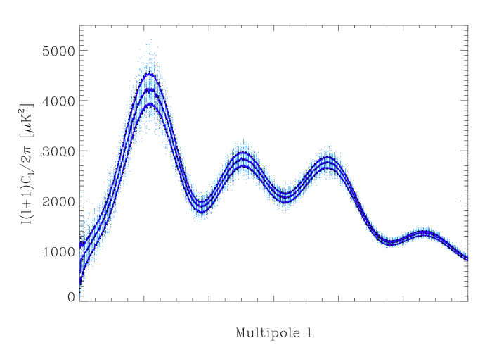
Figure 1: The effect of incomplete sky coverage on the power spectrum estimates. The blue dots are $C_{\ell}/f_{\rm sky}$ extracted from 100 Monte Carlo simulated maps containing only CMB signal, after removing a symmetric strip of $\pm 20^{\circ}$ around the Galactic equator ($f_{\rm sky}=65.8\%$). The black dotted curves are the input theoretical $C_{\ell}$ used in the simulations and the upper and lower $1\sigma$ bounds obtained from Eq. (8). The blue continuous curves are the mean $C_{\ell}$ and upper and lower $1\sigma$ bounds estimated from the MC simulations. This shows that Eq. (8) is a good approximation even when a substantial fraction of the sky is unobserved.

We then decided, for the present paper, to neglect the complications of an exact treatment of the partial sky coverage effect. We emphasize, however, that this does not limit the applicability of the method, since we are able to treat exactly the case of arbitrary sky coverage (for example for very small, irregularly shaped patches, $f_{sky}\ll 1$, as those observed with balloon experiments) by adopting the correct formalism (as done, e.g., by Hivon et al. (2001)).

2.2 Instrumental Noise Contribution to CMB Power Spectrum Measurements

The measurements performed by a given experiment can be thought of as a superposition of sky signal (S) and instrumental noise (N), which are independent statistical processes. When a map is produced from the observations, residual noise is left in the pixelized data. This noise contribution is minimal when a minimum variance map-making (such as the IGLS) is used to obtain the map.

We can write the observation in pixel $p$ as:

$$m_{p}=\sum_{\ell,m}\left(a_{\ell m}^{S}+a_{\ell m}^{N}\right)Y_{\ell m}(\theta_{p},\phi_{p}).$$ (9)

A direct estimation of the power spectrum from such a noisy map would yield:

$$C_{\ell}^{SN}={1\over 2\ell+1}\sum_{m}\left|\left(a_{\ell m}^{S}+a_{\ell m}^{N}\right)\right|^{2}.$$ (10)

Expanding this expression, and averaging over the statistical ensemble, we obtain (due to the independence of the sky and noise processes):

$$\langle C_{\ell}^{SN}\rangle=\langle C_{\ell}^{S}\rangle+\langle C_{\ell}^{N}\rangle.$$ (11)

Thus, an unbiased estimator of $C_{\ell}^{S}$ is:

$$C_{\ell}^{E}=C_{\ell}^{SN}-\langle C_{\ell}^{N}\rangle.$$ (12)

Direct extraction of the angular power spectrum from a map is a relatively quick task, that can be performed in ${\cal N}_{p}^{3/2}\log{\cal N}_{p}$ operations using fast spherical harmonics transforms (Muciaccia et al. 1997; Górski et al. 1999). This facilitates a fast unbiased estimation of the power spectrum through Eq. (12), where the noise bias $\langle C_{\ell}^{N}\rangle$ can be evaluated using Monte Carlo techniques as discussed in the next Section.

It can be easily shown that the rms uncertainty of this power spectrum estimate is:

$$\Delta C_{\ell}^{E}=\left(C_{\ell}+C_{\ell}^{N}\right)\sqrt{2\over(2\ell+1)f_{\rm sky}}.$$ (13)

Note that this uncertainty depends on the unknown ensemble average value $C_{\ell}$. An approximate way of calculating $\Delta C_{\ell}^{E}$ is simply to replace $C_{\ell}$ with the estimate $C_{\ell}^{E}$ in Eq. (13). A more rigorous strategy is to set frequentist confidence intervals by computing the values of $C_{\ell}$ which are consistent with the estimate $C_{\ell}^{E}$ at a given confidence level. We have verified that the two approaches yield nearly identical 1$\sigma$ error bars for $C_{\ell}^{E}$.

3 Results

To determine the noise properties in multipole space, we first apply the IGLS map-making procedure on the TOD, ending up with a minimum variance map of the CMB and an estimate of the true noise properties in time domain. We then produce a number of MC realizations of time streams containing only instrumental noise, where the noise has the statistical properties measured from the data. These simulated time streams naturally incorporate all information about the experiment observational strategy. We apply again the IGLS map-making algorithm to these mock data sets, to construct a set of noise maps. These noise maps have the same statistical properties of the noise which contaminates the real map. They can then be used to characterize the noise statistical properties in multipole space, for example estimating the mean $\langle C_{\ell}^{N}\rangle_{MC}$ to be used in Eqs. (12) and (13).

Figure 2 shows the result of applying this procedure to simulated observations of Planck/LFI 100 GHz channel. The simulations were produced using the standard Planck scanning strategy (i.e. a spinning frequency of 1 r.p.m. and $85^{\circ}$ offset angle between the pointing direction and spin axis of the telescope, with the latter always on the ecliptic) as well as a realistic model of the receiver noise (i.e. $1/f$ noise with $f_{\rm knee}=0.1$ Hz and Planck sensitivity goal, see e.g. Natoli et al. (2002)). A comparison was made with the case of non uniform uncorrelated noise. It is apparent that such a simple model is not accurate enough to characterize the noise properties in multipole space, particularly for small values of $\ell$ ($\ell\mathrel{\mathchoice{\lower 3.6pt\vbox{\halign{$\mathsurround=0pt\displaystyle\hfil#\hfil$\cr<\crcr\sim\crcr}}}{\lower 3.6pt\vbox{\halign{$\mathsurround=0pt\textstyle\hfil#\hfil$\cr<\crcr\sim\crcr}}}{\lower 3.6pt\vbox{\halign{$\mathsurround=0pt\scriptstyle\hfil#\hfil$\cr<\crcr\sim\crcr}}}{\lower 3.6pt\vbox{\halign{$\mathsurround=0pt\scriptscriptstyle\hfil#\hfil$\cr<\crcr\sim\crcr}}}}100$). It is interesting to observe that, since we only need to estimate an average from the Monte Carlo, i.e. the $C_{\ell}^{N}$ to be used in Eqs. (12) and (13), convergence is achieved after a fairly small number of simulations. This is evident from Fig. 2.

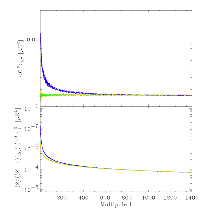
Figure 2: Monte Carlo estimation of the noise properties in multipole space for Planck/LFI. The upper plot shows the average instrumental noise contribution to the power spectrum, $\langle C_{\ell}^{N}\rangle_{MC}$. The blue curve was obtained from 22 realizations of maps containing only instrumental noise with realistic properties (including time correlations); the green curve is from 100 realizations of non uniform uncorrelated noise; the orange curve is from a subset of 22 realizations of the same non uniform uncorrelated noise maps. The simulations were performed using the nominal sensitivity of all combined 34 receivers at 100 GHz, for 7 months of observation. The lower plot shows the noise contribution to the error bars, from the same sets of simulations.

Figure 3 shows histograms of the noise angular power spectrum $C_{\ell}^{N}$, for four multipole values, obtained from $1\,000$ Monte Carlo realizations Planck/LFI maps containing only instrumental noise. In order to speed up the production of simulated maps, we used an inhomogeneous white noise model in place of the correlated noise used in the rest of the paper. This should not alter the results of this test, since the deviation from the white noise behaviour is relevant only at low multipoles (see Fig. 2), where the noise contribution is sub-dominant with respect to the cosmic variance. The comparison with the theoretical distribution, i.e. a $\chi^{2}$ with $(2\ell+1)f_{\rm sky}$ degrees of freedom, shows that use of Eq. (13) yields nearly optimal error bars for the power spectrum estimates.

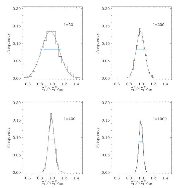
Figure 3: Distribution of the noise contribution in multipole space. The plots show the histogram of $C_{\ell}^{N}$, normalized to its average value, extracted from $1\,000$ Monte Carlo simulations Planck/LFI maps, containing only inhomogeneous uncorrelated instrumental noise, for four values of $\ell$ (from left to right and from top to bottom: $\ell=$50, 200, 400, 1000). Also shown is the $\chi^{2}$ distribution with $(2\ell+1)f_{\rm sky}$ degrees of freedom (continuous line) and the corresponding 1$\sigma$ symmetric error bar, given by $\sqrt{2/((2\ell+1)f_{\rm sky})}$ (blue lines).

Figures 4 and 5 show the results of applying our method to extract the CMB power spectrum from a simulation of Planck/LFI observations at 30 and 100 GHz. In simulating the observations we fully took into account the real Planck scanning strategy. The $85^{\circ}$ offset between the pointing direction and spin axis of the telescope leaves unobserved two areas of about 80 square degrees around the ecliptic poles. We modeled the optical response of the instrument as a symmetric Gaussian beam with FWHM of 33 arcminutes for the 30 GHz detectors and of 10 arcminutes for the 100 GHz detectors. The simulated TOD for the 30 GHz channel has ${\cal N}_{d}\sim 10^{9}$ time samples (14 months of observation), which are mapped into ${\cal N}_{p}\sim 7\times 10^{5}$ pixels. These numbers turn into ${\cal N}_{d}\sim 2\times 10^{9}$ (7 months of observation) and ${\cal N}_{p}\sim 3\times 10^{6}$ for the 100 GHz channel (we remind that IGLS map-making scales approximately linearly with ${\cal N}_{d}$). Going from the simulated data to the power spectrum estimates took about 12 h for the 30 GHz channel, and about 18 h for the 100 GHz channel, using a parallel implementation of the IGLS algorithm running on 16 processors of the Origin 3000 supercomputer at Cineca. These times are dominated by the production of the MC noise maps, 22 in our case. This number is enough to produce good estimates for the average noise contribution (see again Fig. 2). For a detailed discussion about memory requirements, CPU timing, and code scalability of our implementation of the IGLS map-making algorithm, see the paper by Natoli et al. (2001).

Comparison of our $C_{\ell}$ estimates with the theoretical input model yields a $\chi^{2}$/d.o.f. of 1.06 and 1.10 for the 30 and 100 GHz case, respectively. As mentioned in Section 2.1, we also estimated the power ${\cal C}_{b}=\sum_{\ell\in b}\ell(\ell+1)C_{\ell}/2\pi$ in bands $b$ of width $\Delta\ell=20$, in order to reduce small spurious correlation in multipole space. When we use a simple cubic spline algorithm to interpolate these band-power estimates, the resulting curve is nearly undistinguishable from the theoretical input model (see bottom panel in Figs. 4 and 5).

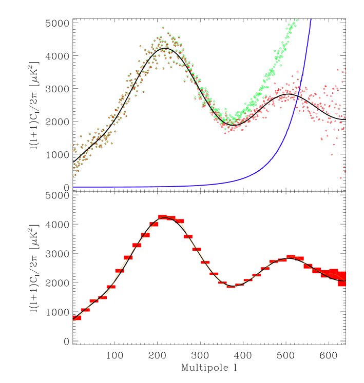
Figure 4: CMB Power spectrum estimation for Planck/LFI 30 GHz channel. The simulated data were produced assuming the nominal sensitivity from all 4 combined radiometers and 14 months of observation (full mission). The top panel shows the power spectrum estimated directly from the map ($C_{\ell}^{SN}$, green points), the MC estimation of the noise contribution ($\langle C_{\ell}^{N}\rangle_{MC}$, blue curve), and the recovered signal power spectrum ($C_{\ell}^{S}$, red points). The bottom panel shows the estimated band-powers ${\cal C}_{b}=\sum_{\ell\in b}\ell(\ell+1)C_{\ell}/2\pi$ and their 1$\sigma$ error bars (red boxes). The orange curve is the result of a cubic spline interpolation of the band-power estimates. In both panels the black curve is the input theoretical model used in the simulation (a COBE-normalized standard CDM).

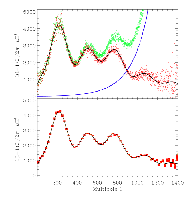
Figure 5: Same as in Fig. 4, but for the 34 combined radiometers of Planck/LFI 100 GHz channel and 7 months of observation (half mission).

4 Conclusions

We have shown that IGLS map-making can be successfully applied, in conjunction with MC techniques, to the problem of estimating the angular power spectrum from CMB maps. The method discussed in this work is fast enough to be already applicable to megapixel maps such as those expected from the Planck Surveyor. No manipulation of the time stream (i.e. high-pass filtering) is required by this method. Furthermore, no unrealistic simplification of the instrumental noise behavior is needed, since the noise properties are estimated directly from the data. Our estimated noise angular power spectrum contains the right information on noise correlation, as well as on the details of scanning strategy, even if we never use explicitly the full pixel covariance matrix. Although we only presented in this paper an application to the case of nearly full-sky maps from the Planck Surveyor, the approach described here can be used for any arbitrary scanning strategy and sky coverage (for example to analyze balloon data), as long as the spectral information on the spatial window of the observation is taken into account.

Finally, we would like to mention a few possible developments of the work described in this paper. We considered a symmetric beam approximation in our analysis. This approximation may prove to be too simplistic when dealing with real experiments. Thus, we are currently generalizing our map-making algorithm to deal with asymmetric beam patterns. We also point out that this power spectrum estimation technique is easily generalizable to CMB polarization maps, since an implementation of the IGLS map-making algorithm for polarization observations exists (see Balbi et al. 2002). We shall discuss this topic in a forthcoming paper.

- (1) Balbi, A., Cabella, P., de Gasperis, G., Natoli, P., & Vittorio, N. 2002, in “Astrophysical Polarized Backgrounds”, eds. S. Cecchini, S. Cortiglioni, R. Sault and C. Sbarra (AIP, New York)
- (2) Bond, J. R., Jaffe, A. H., & Knox, L. 1998, Phys. Rev. D, 57, 2117
- (3) Borrill, J. 1999, in “Proceedings of the 5th European SGI/Cray MPP Workshop”, Bologna, Italy (astro-ph/9911389)
- (4) Doré, O., Teyssier, R., Bouchet, F. R., Vibert, D., & Prunet, S. 2001, A&A, 374, 358
- (5) Doré, O., Knox, L., & Peel, A. 2001, Phys. Rev. D, 64, 083001
- (6) Górski, K. M., Hivon, E. & Wandelt, B. D. 1999 in “Evolution of large scale structure: from recombination to Garching”, ed. by A.J. Banday, R.K. Sheth, L.N. da Costa, (astro-ph/9812350)
- (7) Hobson, M. P., & Magueijo, J. 1996, MNRAS, 283, 1133
- (8) Hivon, E., Górski, K. M., Netterfield et al. 2002, ApJ, 567, 2
- (9) Knox, L. 1995, Phys. Rev. D, 52, 4307
- (10) Mortlock, D. J., Challinor, A. D., & Hobson, M. P. 2002, MNRAS, 330, 405
- (11) Muciaccia, P. F., Natoli, P. & Vittorio, N. 1997, ApJ, 488, 63
- (12) Natoli, P., de Gasperis, G., Gheller, C., & Vittorio, N. 2001, A&A, 372, 346
- (13) Natoli, P., Marinucci, D., Cabella, P., de Gasperis, G., & Vittorio, N. 2002, A&A, 383, 1100
- (14) Netterfield, C. B., Ade, P. A. R., Bock, J. J. et al. 2002, ApJ, 571, 604
- (15) Oh, S. P., Spergel, D. N., & Hinshaw, G. 1999, ApJ, 510, 551
- (16) Scott, D., Srednicki, M., & White, M. 1994, ApJ, 421, L5
- (17) Stompor, R. et al. 2002, Phys. Rev. D, 65, 022003
- (18) Szapudi, I., Prunet, S., Pogosyan, D., Szalay, A. S., & Bond, J. R. 2001, ApJ, 548, L115
- (19) Wandelt, B. D. & Hansen, F. K. 2001 (astro-ph/0106515)
- (20) Wandelt, B. D., Hivon, E. & Górski, K. M., 2001, Phys. Rev. D, 64, 083003