A PERSPECTIVE ON THE CMB ACOUSTIC PEAK
Abstract
CMB angular spectrum measurements suggest a flat universe. This paper clarifies the relation between geometry and the spherical harmonic index of the first acoustic peak (). Numerical and analytic calculations show that is approximately a function of where and are the curvature ( implies an open geometry) and mass density today in units of critical density. Assuming , one obtains where and are the scale factor at decoupling and radiation-matter equality. The derivation of gives another perspective on the widely-recognized - degeneracy in flat models. This formula for near-flat cosmogonies together with current angular spectrum data yields familiar parameter constraints.
1 INTRODUCTION
It has long been recognized that the first peak in the CMB angular spectrum provides information about the curvature of the universe (Doroshkevich, Zel’dovich, & Syunyaev, 1978; Bond et al., 1994; Kamionkowski, Spergel, & Sugiyama, 1994; Efstathiou & Bond, 1999; Cornish, 2000; Weinberg, 2000). The data are now in. TOCO, BOOMERanG, MAXIMA, and DASI have measured the peak position (Miller et al., 1999; Netterfield et al., 2001; Lee et al., 2001; Halverson et al., 2001). Analyses of the data strongly suggest a flat universe (Hu et al., 2001; Jaffe et al., 2000; Stompor et al., 2001; Pryke et al., 2001; Dodelson & Knox, 2000). The MAP satellite, cosmic variance limited through , should make the definitive measurement in the near future (Page, 2000).
As new data resolve higher order peaks, attention shifts to the physics at angular scales beyond that of the first maximum. The object of the present analysis is to clarify the physics derived from the position of the first peak, hereafter called “the peak index” or . The size of the sound horizon at an angular diameter distance to decoupling determines the peak index.111An expression subscripted by ‘*’ or ‘eq’ is evaluated at decoupling or matter-radiation equality respectively. This is widely recognized and serves as a starting point. In Sections 2, 3, and 4, numerical and analytic calculations yield the peak index as a function of and . All results are checked with CMBFAST (Seljak & Zaldarriaga, 1996). In Section 5, a simple formula for , applicable to low universes, is developed alongside geometric and classical interpretations of the formal results. It is found that the peak index approximates a function of . Although our analysis grounds itself in the familiar concepts of and , the results are not widely recognized. While the physical effects responsible for are understood, the interplay that gives the dependence is not intuitive and holds a number of surprises. We end the investigation by using the functional form of and current angular spectrum data to obtain parameter constraints resembling those of more sophisticated treatments.
Throughout this work, the (,) plane serves as the parameter space. Other quantities enter, though the relation between and is relatively independent of them. To be concrete, we take , consistent with nucleosynthesis (Burles, Nollett, & Turner, 2001). The redshift of decoupling, , is taken as 1400 from the Saha equation. The Hubble constant assumes 72 km/s/Mpc in accord with the HST Key Project results (Freedman et al., 2001).
2 ANGULAR DIAMETER DISTANCE
The comoving Friedmann-Robertson-Walker (FRW) metric for a closed universe () may be written as
| (1) |
where denotes conformal time, , and is the line element of a unit two-sphere. All spacetime intervals are given in units of . The angular diameter distance to an object of proper length at comoving distance () is defined so that .
| (2) |
where is the solution to the Friedmann equation:
| (3) |
Flat and open geometries are treated analogously.
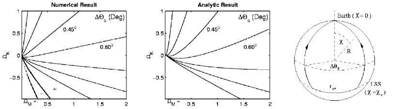
Numerical Result can be evaluated numerically. The distance to redshift 1400 is computed for models across the plane using cosmography routines from David Hogg (Hogg, 1999).
3 THE SOUND HORIZON
Sound travels through a tightly coupled photon-baryon system with speed
| (6) |
where Q is 3/4, and and are the energy densities of baryons and radiation, respectively. The sound horizon at decoupling in comoving coordinates is then
| (7) | |||||
(Hu & Sugiyama, 1996). Note that curvature does not affect sound dynamics before decoupling. In any geometry, will be the same.
4 THE HORIZON ANGLE AND THE PEAK INDEX
and give the angular size of the horizon:
| (8) |
Values for corresponding to the numerical and analytic results for (see Section 2) are plotted in Figure 1. Curves of constant approximate straight lines, which intersect the origin of the () plane. The angle subtended by the sound horizon, and so the position of the first peak, approximates a function of . A well known corollary to this general statement is that a peak corresponding to should be insensitive to variations in (Bond et al., 1994; Hu et al., 2001).
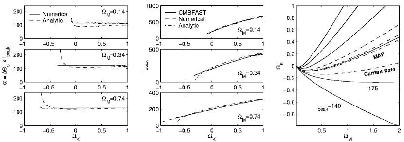
To check whether this simple analysis agrees with the standard model, we compare the above results to those from CMBFAST (Seljak & Zaldarriaga, 1996). CMBFAST calculates the CMB angular spectrum.222CMBFAST inputs are ,recfast,no reion, scalar only,primordial index 1,adiabatic). Then, from the spectrum multiplies from Figure 1 to give the constant of proportionality . As shown in Figure 2, the numerically derived increases from 110 () to 125 () and has weak if any dependence on curvature. The near constant graphs of suggests a well-defined agreement between the peak indices from CMBFAST and those derived from this work’s numerical and analytic calculations (see middle frame of Figure 2).
5 DISCUSSION
To gain intuition about , consider the closed comoving universe (eq. [1]) illustrated in Figure 1, where time and azimuthal angular coordinates have been supressed to produce the familiar two-sphere geometry. In this picture, CMB photons follow great circles, and, assuming a small angle, derives from inspection: which is exactly equation (8).
To better understand the parameter dependence of , take the sound speed (eq. [6]) to be constant at . (With and radiation density derived from the COBE FIRAS measurement, the sound speed decreases at a near constant rate () from at a=0 to four-fifths that value at decoupling (Fixen et al., 1997).) The sound horizon is then
| (9) |
where the final equality follows from the Friedmann equation (3) with .
To obtain a simple formula for , expand to first order in :
| (10) |
The expansion applies to models with a low curvature-to-matter ratio. Coincidentally, such models are favored by experiment, so that the resulting formula for is useful. Given equations (9) and (10) and a value of from Figure 2,
| (11) |
This near-flat approximation is plotted in Figure 2 where . For flat models, the distance to last scatter (eq. [10]) scales as . One may intuit that self-gravitation leads to smaller cosmological separations. This same “gravitational” effect decreases the distance between the big bang and last scatter, and therefore (eq. [9]) also scales with an overall factor of . In equation (11), the dependence of cancels that of . This cancellation helps explain the - degeneracy of flat cosmogonies. Furthermore, the term in equation (11) is proportional to the curvature times the area between light rays in a two-dimensional representation of an universe (e.g. Figure 1). This suggests that one may think of (,) dependence of in near-flat spacetimes as resulting from light curving like the geodesics of a two-dimensional space of constant curvature. Finally, the effect of radiation on early universe dynamics and, in particular, on is made explicit by the appearance of in equation (9). Radiation-dominated cosmological growth per expansion scale () is less than that of matter-dominated dynamics. In low universes, radiation brings last scattering even closer to the big bang and so shortens . Thus, the effect of radiation in the early universe is to spoil the pure dependence of as manifest by the curved contours in the plot of equation (11) in Figure 2. The straightness of the contours is restored in the numerical result shown in Figure 1. This suggests that explicit inclusion of in the computation of balances the dependence of .
6 CONCLUSION
The peak index has long been recognized as an indicator of geometry. It is hoped that the present analysis sheds new light on . The peak index does not determine the magnitude of curvature, but rather the ratio of curvature to matter. A measurement of the peak’s angular scale gives the precise geometry only if , otherwise is a function of . Furthermore, in deriving the dependence of , unexpected cosmological cancellings were discovered. Particularly useful is the balance of overall matter dependencies in and which helps account for the - degeneracy in flat models. At the same time, however, it is remarkable that the admittedly simple arguments of this work yield such a decisive cosmological indicator. Within the next few years, NASA’s MAP satellite data should give to cosmic-variance levels. This measurement will burn a sharp line of possible worlds across the () plane.
References
- Bond et al. (1994) Bond, J.R., Crittenden, R., Davis, R.L., Efstathiou, G., & Steinhardt, P.J. 1994, Phys. Rev. Lett., 72, 13
- Burles, Nollett, & Turner (2001) Burles, S., Nollett, K.M., & Turner, M.S. 2001, ApJ, 552, L1
- Cornish (2000) Cornish, N.J. 2000, preprint(astro-ph/0005261)
- Dodelson & Knox (2000) Dodelson, S., & Knox, L. 2000, Phys. Rev. Lett., 84, 3523
- Doroshkevich, Zel’dovich, & Syunyaev (1978) Doroshkevich, A.G., Zel’dovich, Ya.B., & Syunyaev, R.A. 1978, Sov. Astron., 22, 523
- Efstathiou & Bond (1999) Efstathiou, G., & Bond, J.R. 1999, MNRAS, 304, 75
- Fixen et al. (1997) Fixen, D.J., Hinshaw, G., Bennet, C.L., and Mather, J.C. 1997, ApJ, 486, 623
- Freedman et al. (2001) Freedman, W.L., et al. 2001, ApJ, 553, 47
- Halverson et al. (2001) Halverson, N.W., et al. 2001, ApJ, submitted (astro-ph/0104489)
- Hogg (1999) Hogg, D.W. 1999, preprint(astro-ph/9905116)
- Hu & Sugiyama (1996) Hu, W., & Sugiyama, N. 1996, ApJ, 471, 542
- Hu et al. (2001) Hu, W., Fukugita, M., Zaldarriaga, M., & Tegmark, M. 2001, ApJ, 549, 669
- Jaffe et al. (2000) Jaffe, A.H., et al. 2000, Phys. Rev. Lett., 86, 3475
- Kamionkowski, Spergel, & Sugiyama (1994) Kamionkowski, M., Spergel, D.N., & Sugiyama, N. 1994, ApJ, 426, L57
- Knox & Page (2000) Knox, L., & Page, L.A. 2000, Phys. Rev. Lett., 85, 1366
- Knox, Christensen, & Skordis (2001) Knox, L., Christensen, N., & Skordis, C. 2001, ApJ, 563, L95
- Lee et al. (2001) Lee, A.T., et al. 2001, ApJ, 561, L1
- Miller et al. (1999) Miller, A.D., et al. 1999, ApJ, 524, L1
- Netterfield et al. (2001) Netterfield, C.B., et al. 2001, ApJ, in press (astro-ph/0104460)
- Page (2000) Page, L.A. 2000, in Proc. IAU Symposium 201, ed. A. Lasenby & A. Wilkinson, in press (astro-ph/0012214)
- Peebles (1993) Peebles, P.J.E. 1993, Principles of Physical Cosmology, (Princeton University Press)
- Pryke et al. (2001) Pryke, C., Halverson, N.W., Leitch, E.M., Kovac, J., Carlstrom, J.E., Holzapfel, W.L., & Dragovan, M. 2001, ApJ, submitted (astro-ph/0104490)
- Seljak & Zaldarriaga (1996) Seljak, U., & Zaldarriaga, M. 1996, ApJ, 469, 437
- Stompor et al. (2001) Stompor, R., et al. 2001, ApJ, 561, L7
- Weinberg (2000) Weinberg, S. 2000, Phys. Rev. D, 62, 127302