Joint Cosmic Shear Measurements with the Keck and William Herschel Telescopes

Abstract

The recent measurements of weak lensing by large-scale structure present significant new opportunities for studies of the matter distribution in the universe. Here, we present a new cosmic shear survey carried out with the Echelle Spectrograph and Imager on the Keck II telescope. This covers a total of 0.6 square degrees in 173 fields probing independent lines of sight, hence minimising the impact of sample variance. We also extend our measurements of cosmic shear with the William Herschel Telescope (Bacon, Refregier & Ellis 2000) to a survey area of 1 square degree. The joint measurements with two independent telescopes allow us to assess the impact of instrument-specific systematics, one of the major difficulties in cosmic shear measurements. For both surveys, we carefully account for effects such as smearing by the point spread function and shearing due to telescope optics. We find negligible residuals in both cases and recover mutually consistent cosmic shear signals, significant at the $5.1\sigma$ level. We present a simple method to compute the statistical error in the shear correlation function, including non-gaussian sample variance and the covariance between different angular bins. We measure shear correlation functions for all fields and use these to ascertain the amplitude of the matter power spectrum, finding $\sigma_{8}\left(\frac{\Omega_{m}}{0.3}\right)^{0.68}=0.97\pm 0.13$ with $0.14<\Omega_{m}<0.65$ in a $\Lambda$CDM model with $\Gamma=0.21$. These $68\%$ CL uncertainties include sample variance, statistical noise, redshift uncertainty, and the error in the shear measurement method. The results from our two independent surveys are both consistent with measurements of cosmic shear from other groups. We discuss how our results compare with current normalisation from cluster abundance.

1 Introduction

Weak gravitational lensing of background galaxies by intervening large-scale structure (‘cosmic shear’) provides direct information about the total mass distribution in the universe, regardless of its nature and state. A measurement of cosmic shear thus bridges the gap between theory, which is primarily concerned with dark matter, and observation, which generally probes only luminous matter. The recent measurements of coherent distortion of faint galaxies by several groups (van Waerbeke et al. 2000; Bacon, Refregier & Ellis 2000 [BRE]; Wittman et al. 2000; Kaiser, Wilson & Luppino 2000; Maoli et al. 2001; Rhodes, Refregier & Groth 2001; van Waerbeke et al 2001; Hämmerle et al. 2001; Hoekstra et al. 2002; Refregier, Rhodes & Groth 2002) has triggered great interest in the provision of new constraints on the amount and distribution of dark matter, together with measurements of several cosmological parameters.

If intrinsic galaxy orientations are essentially random in a given survey (which requires the survey to be sufficiently deep; see Brown et al. 2000; Catelan et al. 2000; Heavens et al 2001; Croft & Metzler 2001; Crittenden et al 2001), any coherent alignment must arise from distortion due to weak lensing. Light paths from galaxies projected close together on the sky pass through, and are gravitationally distorted by, the same dark matter concentrations. This coherent distortion contains valuable cosmological information (eg. Bernardeau et al. 1997; Jain & Seljak 1997; Kamionkowski et al. 1997; Kaiser 1998; Hu & Tegmark 1998). In particular, the variance of the distortion field measures the amplitude of density fluctuations ($\sim\sigma_{8}\Omega_{m}^{0.5}$). This shear measurement is free from assumptions about gaussianity or the $M-T$ relation, and whilst the shear-based measurement is currently comparable in precision to that from local cluster abundance, further progress is limited solely by the number of fields observed.

The validity of results from cosmic shear surveys depends sensitively on the treatment of systematic errors. A further issue arises from sample (or ‘cosmic’) variance, the impact of which can be limited by using numerous independent sightlines to complement panoramic imaging of a few selected areas. With these motivations in mind, we present a comparison of the cosmic shear observed with two independent instruments (Keck and WHT), using two different survey strategies.

In this paper, we describe the first cosmic shear measurements with the $8^{\prime}\times 2^{\prime}$ Echelle Spectrograph and Imager (ESI) on the Keck II telescope. This Keck survey reaches a depth of $z\simeq 1.0$, comparable to other recent cosmic shear surveys (e.g. van Waerbeke et al 2001, Bacon et al 2000). However, the much faster acquisition of fields with ESI in comparison to 4m telescopes such as the William Herschel Telescope allows us to obtain very many more fields (173 in the final survey). This improves the cosmic shear signal measured, by minimising the contribution to noise of the sample variance, i.e. the error upon the mean lensing signal resulting from the measurement of shear on only a limited number of lines of sight. In order to measure the cosmic shear signal, we analyse the correlation function of the shear on various scales, and obtain constraints on cosmological parameters using a $\chi^{2}$ fit to theoretical predictions upon varying these parameters.

In addition to this investigation, we extend our original detection of cosmic shear on the 4.2m WHT (in BRE), to a measurement of the correlation function of the distortion field for this dataset. A more precise measurement is afforded by the increase in the number of WHT fields to a total of 20, with a further increase in area due to the larger $16^{\prime}\times 16^{\prime}$ size of field with the new WHT mosaic camera.

This paper is organised as follows. In §2 we discuss our observational strategy for measuring cosmic shear with both telescopes. We then describe (§3) the procedure for observing with the Keck telescope, and explain the method used for reducing the data. We follow this by a treatment of the systematic effects associated with the Keck data, such as shear distortion from the camera and the anisotropic smear due to telescope tracking.

Having dealt with the Keck data up to the stage of measuring galaxy shapes, we review the procedure for obtaining the WHT data in §4, followed by the approach adopted for data reduction and removal of systematic effects.

We proceed to develop the correlation function formalism in §5, which we use for precision measurements of the cosmic shear, in §6. We then interpret the shear signal in terms of cosmological models in order to obtain limits on the cosmological parameters $\sigma_{8}$ and $\Omega_{m}$. Our conclusions are summarised in §7.

2 Survey Strategy

The aim of our Keck and WHT surveys has been to acquire deep ($z\simeq 1$) fields representing numerous independent lines of sight, sufficiently scattered to sample independent structures and thus minimise uncertainties due to sample variance. These lines of sight must be chosen in a quasi-random fashion, without regard to the presence or absence of mass concentrations, in order to obtain a representative sample of the mass fluctuations in the universe. Here we describe the strategy adopted for the two surveys, based on that in BRE.

The survey fields for both Keck and WHT were selected by choosing a sparse ($>2^{\circ}$ separation for statistical independence) grid of coordinates spanning the range accessible to the telescope at a given time. We tuned the Galactic latitude of the grid to ensure $\sim$50 unsaturated stars within the Keck field of view, and $\sim$200 in the WHT fields, so that the anisotropic PSF and the camera distortion could be carefully mapped (see below). The STScI Digitised Sky Survey was then used to find an appropriate final field near each set of coordinates, avoiding stars brighter than $R<11$ in the APM and GCC catalogues, to prevent large areas of saturation or ghost images.

As a final constraint, each field was observed within $20^{\circ}$ of zenith for both telescopes. This minimises smearing due to atmospheric refraction for Keck, which does not have an Atmospheric Dispersion Corrector (see section 6 and figure 10 for confirmation that this is not a limiting systematic). For both telescopes the constraint minimises any image distortion associated with telescope or instrument flexure. Figure 1 shows the positions of the resulting selected survey fields on the sky.

We must now determine the depth to which to observe these fields. We have shown in BRE that the cosmic shear signal is measurable with WHT images having a 1 hour exposure length, corresponding to a usable galaxy sample with median source redshift $z_{s}=0.8$. We have further demonstrated in Bacon et al (2001) that longer exposures do not improve the signal greatly, as beyond this depth galaxy shapes are seriously degraded by a typical ground-based PSF. On the other hand, shorter exposures face the danger of considerable contamination by intrinsic alignments of galaxies (e.g. Heavens et al 2001). We therefore aimed to probe the same redshift range with our new Keck survey. An exposure time of 10 minutes was calculated to allow $5\sigma$ detections of point sources at $R=26$, given the optics throughput, sky background in the Keck $R$ filter frequency range and the quantum efficiency of the ESI CCD. However, as we shall see, the better seeing during our observations with Keck results in a slightly fainter magnitude limit than the WHT survey; this is entirely acceptable, as we can compare results by scaling the predictions according to the equation $\sigma_{\gamma}\propto z^{0.8}$ (see e.g. BRE).

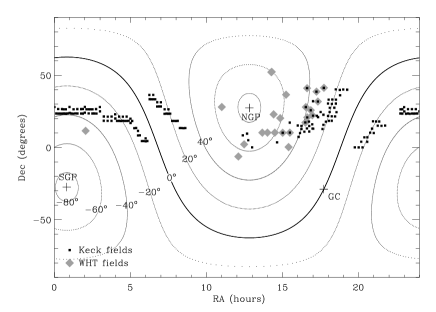
Figure 1: The sky location of the cosmic shear fields. Galactic latitudes of $0^{\circ}$, $\pm 20^{\circ}$, $\pm 40^{\circ}$, $\pm 60^{\circ}$ are shown as contours; the Galactic centre and poles are shown as a cross.

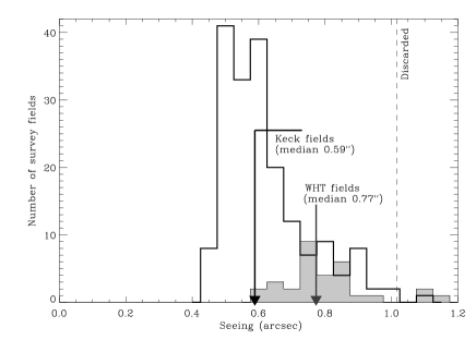
Figure 2: Histogram of seeing (FWHM) in all survey shear fields after stacking dithered exposures. Keck data are shown in white; WHT data are shown as shaded. Each $8^{\prime}\times 16^{\prime}$ WHT chip is counted separately. Combining survey area from the two telescopes, the median seeing is 0.73”; no data with seeing worse than 1” is used.

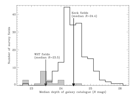
Figure 3: Median reddening-corrected $R$-band magnitude of the galaxies in each field that are used in the final object catalogue. The median depth of the combined surveys is $R$=24.0.

The fact that gravitational lensing is achromatic permits us a free choice of photometric band for our observations. However, we should note that $R$ and $I$ afford the most efficient deep imaging in a given exposure time. Due to fringing in the $I$ band with the EEV CCD in use at the WHT, we choose to image in $R$ with both telescopes. The Keck $R$-band is a specially constructed filter with similar throughput and spectral range to the WHT Harris $R$; the slightly different galaxy distribution probed by this filter is taken into account later in our redshift uncertainty estimates.

3 Keck data

3.1 Observations

As we briefly mentioned above, the great advantage which Keck presents in measuring cosmic shear is its speed in achieving the necessary depth; 10 minute exposures reach $R=26$ (contrast the 1 hour necessary for such a depth with WHT). We can therefore obtain very many independent lines of sight per night, thus reducing the impact of sample variance.

We observed 173 $2^{\prime}\times 8^{\prime}$ ESI fields using a specially made $R$ filter ($\bar{\lambda}=6657$Å, effective FWHM$(\lambda)=1200$Å), over the course of 6 nights in June 2000, November 2000 and May 2001. The necessary imaging observations were done as a good seeing override on an independent spectroscopic programme. The pixel size of $0.153^{\prime\prime}$ for ESI is considerably finer than that for WHT, allowing better sampling of the galaxy images.

For each of our fields, three separate exposures were taken, each offset by $5^{\prime\prime}$. This enables the continual re-calibration of optical distortions in the telescope and camera (see section 3.3), and the removal of cosmetic defects and cosmic rays. All the fields were observed as they passed near the meridian (in order to minimise image distortion from the atmosphere and from telescope or instrument flexure) but no closer than 5^∘ to zenith (to minimise sky rotation and potential tracking errors on this alt-az telescope). Bias frames, sky flats and dome flats were acquired at the start and end of each night, and standard star observations were taken regularly throughout each night. The telescope was focused several times per night to minimise camera distortions.

As exposures were observed, we used our real-time SExtractor-based (Bertin & Arnouts 1996) software on recently completed exposures in order to monitor PSF size and stellar ellipticity. Figure 2 records the seeing values for all fields; we found that the median seeing for the observations was $0.59^{\prime\prime}$, with 75% in seeing better than $0.7^{\prime\prime}$. As we discuss below, this excellent quality data yields a low level of noise on the estimates of cosmic shear.

Furthermore, the rms stellar ellipticity for the images was $\sigma_{e*}=0.035$. This relatively low value facilitates the necessary PSF corrections (see e.g. Bacon et al 2001, Erben et al 2001). The stellar ellipticity on Keck fields is often found to be due to tracking errors, seen as a uniform PSF anisotropy across the field of view (see figure 5 for an example and discussion in $\S$3.4). In exposures with excellent tracking, the dominant effect appears to be astigmatism due to the fact that the CCD is slightly skewed with respect to the focal plane, thus probing optical conditions slightly above and below the focus.

In terms of depth, with magnitudes calibrated using photometric standards, we found that the median magnitude of all galaxies detected was $R$=25.1, with an imcat signal-to-noise of 5.0 being reached for galaxies at $R$=25.8. We keep $\simeq 27.5$ resolved galaxies per square arcminute in our final object catalogue (see section 3.4 for the selection criteria), which corresponds to a final magnitude median of $R\simeq 24.4\pm 0.2$, including reddening corrections. The distribution of magnitudes for the final galaxy catalogue extends substantially fainter than this median, with the galaxy count as a function of magnitude dropping to 50% of maximum at $R=25.2$. According to e.g. Cohen et al (2000), our median magnitude of $R=24.4$ corresponds to a median source redshift of $z_{s}\simeq 1.0$. We can estimate the error on this by taking Cohen et al’s measured interquartile range of redshifts for galaxies at this magnitude, $IQ$=1.6-0.55=1.05, and using the estimate of the error on the mean for a gaussian distribution, $\sigma=IQ/(1.35\sqrt{n})=0.1$, where the number of galaxies with redshifts measured $n=49$. Thus we will use an estimate of the median redshift $z_{s}=1.0\pm 0.1$. This quantity may be subject to additional sample variance, which would increase the error; we will therefore quote our redshift error separately to other statistical errors for comparison with future redshift surveys.

3.2 Data Reduction

These deep images were reduced following standard methods. Bias subtraction of the science exposures and sky-flats was individually calibrated for each image using the overscan regions at the edge of the chip. The science exposures were then trimmed and divided by a median composite (with 3$\sigma$ clipping) of the flat fields for a given night. To eliminate any remaining background gradients, the science images were also divided by a stack of all the (median-normalised) exposures from that night. In contrast to the WHT data, no fringing is observed on the ESI images, due to a thicker CCD than that for the WHT camera; this simplifies the reduction considerably.

The multiple exposures for each field were aligned by cross-matching common objects in SExtractor catalogues (Bertin & Arnouts 1996). Typically $\simeq$250 objects were found in common per Keck field, thus providing a stringent estimate of the mean dither offset (to 0.02 pixel accuracy). The exposures were then shifted by the required non-integer number of pixels via a linear interpolation using the IRAF imshift routine. As we discuss below in §3.3, rotations between dithers, and astrometric distortions due to the telescope and camera optics, are found to be negligible in our analysis.

The resulting registered exposures were then divided by their median values to normalise their background levels and averaged with 3$\sigma$ clipping to remove cosmic rays and cosmetic defects. Remaining problematic areas (edges, bad columns, regions containing light leaks from stars outside the field of view, spikes from slightly saturated stars, and a $<1^{\prime}$ square unresponsive region in the corner of the CCD) were flagged and are not used in our cosmic shear analysis (see also $\S$3.5). Note that saturation spikes are also largely excluded from our object catalogues by an initial $e<0.5$ cut, but a local sky background gradient required that a few galaxies within 2” of bright stars also be discarded. Fortunately with the small field of ESI we can selectively avoid most stars which are bright enough to saturate. After these maskings, a reliable $\sim$12.8 square arcminutes per survey field remains.

Having obtained carefully reduced data, the next step is to catalogue the shapes of galaxies and to estimate their gravitational shear. In order to do this, we must correct for any shear introduced by the telescope itself, together with tracking errors and atmospheric smearing which convolve the galaxy shapes: these effects can mimic a coherent distortion which must be removed. We first turn to the issue of instrumental optical distortions, mimicking shear.

3.3 Instrumental Distortions

Our method for determining the shear field induced by the telescope and camera, using the offsets in SExtractor catalogues of our dithered astrometric frames, is fully documented in BRE. Figure 4 shows the ESI instrumental shear pattern obtained using this method, averaging over 20 fields in order to overcome noise, as the error on the shear is 0.09 in a $1^{\prime}$ square bin on a given field. We find after this averaging that the shear has a mean of $0.2\%$ and is $<0.3$% everywhere; the shear measured fluctuates by $<0.1$% as we average over different sets of fields. This implies that, since our results deal with shears of $\sim$ 1%, and since these intrinsic values add in quadrature to negligibly affect these shears, we can neglect this effect in our analysis. (Note that the ESI field has an illuminated area which is rotated from the $x-y$ axes by $7^{\circ}$, accounting for the slightly slanted geometry on this figure.) The magnification and rotation components were also found to be $<0.3$%, and are consequently negligible over such a small field.

Figure 4: Example instrumental shear pattern for ESI. Each bar represents the magnitude and orientation of astrometric distortions averaged over 20 sets of three dithered exposures. The illuminated area of the CCD is rotated from the $x-y$ axes by $7^{\circ}$, accounting for the occupied bins seen here.

3.4 Point Spread Function

We now turn to more important sources of systematic error which need correction: the isotropic smearing of images due to the atmosphere and telescope optics, together with anisotropic smearing due to tracking errors, dither alignment and optics.

We used Kaiser’s imcat software (Kaiser et al 1995) to detect objects on our images, and measure ellipticity, radius, magnitude and polarisability (responsiveness to image shear/smear; a large galaxy will be less affected by a given smear than a small galaxy) for each object. Our procedure is described in detail in BRE.

Figure 5: Example stellar ellipticity pattern for ESI. (Left) Before correction; the pattern varies qualitatively between fields but mean ellipticity here is typical of the field-to-field average of 0.035. (Right) After correction; mean ellipticity reduced to $<$0.001 across the survey, with residual orientations essentially randomised.

Noisy detections in our imcat hfindpeaks catalogues were removed using criteria as in BRE ($r_{g}>1.0,\nu>15,e<0.5$). Note that after this, all objects are weighted equally. The stars to be used to monitor the PSF were selected from the non-saturated locus on a magnitude-radius plane for each field. In most observations, the distribution of stellar ellipticities over the field is found to be smooth and slowly varying (see figure 5 for an example). Some exposures taken during July 2000 were found to have an unexplained, sharp discontinuity in this pattern $\frac{2}{3}$ of the way up the field. For these fields, only objects on one side of the PSF discontinuity were used. The rms field-to-field stellar ellipticity over all used Keck data was found to be $\sigma_{e*}\simeq 0.035$; and reduced to a negligible $<$0.001 by our analysis.

We then measured shear estimators for each galaxy and corrected them for convolution with the local PSF as described in BRE. To interpolate the PSF to the position of each galaxy, we iteratively spatially fitted the measured stellar ellipticities with a 2-D polynomial, removing extreme outliers due to noise and blended images. Similarly, each component of the smear polarisability tensor $P^{*}_{sm}$ was fitted with a 2-D polynomial. Although individually smooth, the PSF patterns were found to have large variations from field to field. The degree of fitting polynomial was thus adapted to suit each pattern. Typically, a quadratic or cubic component was necessary in the $y$ direction; the much more narrow $x$ direction generally required only a constant or linear function. We avoided high-order polynomial PSF models which diverged towards the edges of the field and would have spuriously elongated galaxies by over-correcting for the true PSF smearing effect (see Massey et al. 2001).

Figure 6: Average shear of all galaxies in all Keck fields as a function of position on chip. Overall, $\langle\gamma_{1}\rangle~{}=-0.02\%\pm 0.16\%$ and $\langle\gamma_{2}\rangle~{}=-0.29\%\pm 0.16\%.$

3.5 Masking of the Field

As a check for systematic effects associated with data reduction or chip behaviour, we took shear estimators from all galaxies in all fields and averaged as a function of CCD position (see figure 6). We find that the mean shear for our entire ensemble is $\gamma_{1}=-0.0002\pm 0.0016$ and $\gamma_{2}=-0.0029\pm 0.0016$. This is consistent with zero offset in the whole ensemble, as we would expect. Figure 6 further demonstrates that there is no significant structure in our shear values with position on the chip.

This plot proved very helpful to expose problems with the different parts of the analysis (see discussion in Massey et al. 2001) . In particular, the necessity for stringent masking of the field (see also §3.2) quickly became manifest. The plot not only mirrored the locations of obvious CCD defects, but also indicated which other regions of the chip were unsuitable for high-precision shape measurements. In particular, galaxies at the edges of the data/mask are cut apart by the image and appeared aligned with the boundary. This caused a 2% mean shear offset inside ESI’s long and thin field geometry. Other galaxies also appeared spuriously aligned in regions where flat-fielding of any of the three dithered exposures was imperfect (e.g. near the edge of any one of the dithers; near internal reflections of bright stars outside the field of view; or through cirrus). In these instances, the dithers have slightly different background levels and image co-addition leads to residual ellipticities in galaxies around these locations. If they are not excluded, the mean shear throughout the field is again offset by $\sim$1%. we found that the masking of approximately one quarter of the CCD reduced these effects to negligible levels in $\sim$12.8 square arcminutes of selected data per field.

4 WHT data

4.1 Observations

The WHT data used includes the 13 $8^{\prime}\times 16^{\prime}$ fields used in our previous detection of cosmic shear (BRE), as well as 7 fields observed in June 2000 with the new larger field of view for the Prime Focus Camera ($16^{\prime}\times 16^{\prime}$). Thus the total area of the combined WHT survey is 1.0 square degree.

The fields were observed using the Harris $R$ filter with the William Herschel Telescope Prime Focus Camera. The $16^{\prime}\times 16^{\prime}$ field has a pixel size of $0.24^{\prime\prime}$; for each field four dithers were observed, each offset by $5^{\prime\prime}$ in order to estimate telescope shear estimation and to remove cosmetic defects. As for the Keck survey, we observed the fields as they passed through meridian to minimise flexure-induced distortions. Bias frames, sky flats and standard stars were acquired each night, and refocusing was carried out several times per night.

The median seeing for the WHT fields is $0.8^{\prime\prime}$, which is adequate for our purposes (see Figure 8 of Bacon et al 2001); Figure 2 records the seeing values for all fields. No data was used with seeing $>1.0^{\prime\prime}$.

The dithers were exposed for 900 seconds each, amounting to a 1 hour exposure on each field. The median magnitude of detected galaxies was $R$=25.0, with an imcat signal-to-noise of 5.0 being reached for galaxies at $R$=25.8, similar to our previous survey fields. We keep 15 resolved galaxies per square arcminute in our final object catalogue (see section 3.4 for the selection criteria), which corresponds to a final magnitude median of $R\simeq 23.5\pm 0.2$, including reddening corrections. As with Keck, the distribution of magnitudes for used galaxies extends substantially fainter than the median, with the galaxy count as a function of magnitude reaching 50% of maximum at $R=24.4$. Figure 3 records the reddening-corrected median magnitude vs number densities for all fields. According to e.g. Cohen et al (2000), the above median magnitude corresponds to a median source redshift of $z_{s}\simeq 0.8$; using a similar estimate for the redshift error to that in section 3.1, we find an uncertainty in this quantity of 0.06. As this may be subject to sample variance, we will conservatively use a rounded uncertainty of 0.1.

4.2 Data Reduction

The reduction of the WHT fields followed the same standard procedure as outlined in BRE and §3.2 above. Bias subtraction and flat fielding were followed by the elimination of fringing, which occurs on the fields at 0.5% of sky background level. In order to defringe, all science exposures for each night were stacked without offsetting, using sigma-clipping to remove objects; this provided a fringe frame for each night. A multiple of the fringe frame which minimised rms background on each dither was subtracted, resulting in the fringes being reduced to an $<0.05$% level, as in BRE. Astrometric matching and stacking of dithers then proceeded in the same manner as for the Keck data.

4.3 Instrumental Distortions

We re-checked the instrumental distortion for the WHT fields using the same method as for the Keck fields (see §3.3 and BRE). However, the larger number of objects in common in the WHT exposures affords a determination of the instrumental shear on individual fields rather than having to stack many fields as we did in 3.3. Figure 7 shows the WHT instrumental shear pattern for a typical field, including both chips of the new $16^{\prime}\times 16^{\prime}$ mosaic field. Since the shear has a mean of $0.1\%$ and is $<0.4$% at the edges of the field, we again find that the correlation function of the telescope shear is negligible and need not be corrected for. The telescope shear estimates fluctuate by $<0.1$% from field to field. Magnification and rotation components are also found to be $<0.4$%, and are therefore negligible.

Figure 7: Example of astrometric distortions for both chips of the Wide Field Camera on WHT.

4.4 Point Spread Function

Correction for isotropic and anisotropic smear components proceeded in an entirely analogous fashion to that for the Keck data, using imcat’s ellipticities and polarisabilities to correct the galaxy shear estimates (see BRE for full details). The same criteria were used for removing noisy detections ($r_{g}>1.0,\nu>15,e>0.5$). The rms ellipticity of our stars from field to field was $\sigma_{e*}\simeq 0.05$ (see BRE figure 7 for an example stellar ellipticity field).

As with the Keck data, we checked for systematics in our shear estimators by taking all shear estimators from all fields and averaging them as a function of position (Figure 8). For WHT we find that the mean shear for our entire ensemble is $\gamma_{1}=0.0000\pm 0.0013$ and $\gamma_{2}=0.0007\pm 0.0013$. This is entirely consistent with zero offset in the whole ensemble, as we would expect. Similarly, the figures demonstrate that there is no significant dependence of our shear values on position on the chip.

Figure 8: Average shear of all galaxies in all WHT fields as a function of position on chip. Overall, $\langle\gamma_{1}\rangle~{}=0.00\%\pm 0.13\%$ and $\langle\gamma_{2}\rangle~{}=0.07\%\pm 0.13\%.$

5 Cosmic Shear Statistics: The Correlation Function

We are now in possession of good quality, wide area data for cosmic shear estimation from two telescopes. How are we to best extract the information contained from our shear estimator catalogues, in order to estimate cosmological parameters and the amplitude of the mass power spectrum?

In this paper we choose to use the shear correlation function (e.g. Kaiser 1998; Kamionkowski et al 1998), a useful probe of the shear power on various scales. It has the advantage of being simply related to the shear power spectrum by a Fourier transform, and affords precise checks of the contribution to our results of PSF anisotropy systematics. In this section, we shall describe the correlation functions and their use as estimators for the shear signal.

The material which we have to work with is a set of catalogues containing the positions of galaxies, plus the shear estimator associated with each one; we therefore have a set of noisy samples of the cosmic shear field $\gamma_{i}({\mathbf{\theta}})$. For this field, we can define shear correlation functions in the following way:

$$C_{1}(\theta) \equiv \langle\gamma_{1}^{r}(0)\gamma_{1}^{r}(\theta)\rangle$$

$$C_{2}(\theta) \equiv \langle\gamma_{2}^{r}(0)\gamma_{2}^{r}(\theta)\rangle,$$ (1)

where the average is to be taken over all galaxy pairs separated by an angle $\theta$. In practice, of course, we will average over an annulus $[\theta,\theta+\Delta\theta]$. Note that all objects that pass the initial selection cuts (see §3.5) are given equal weight. The shears used are those for a rotated coordinate system, where the $x$-axis is defined by the line joining the two galaxies. This can be achieved using the transformations

$$\gamma_{1}^{r} = \gamma_{1}\cos(2\phi)+\gamma_{2}\sin(2\phi)$$

$$\gamma_{2}^{r} = -\gamma_{1}\sin(2\phi)+\gamma_{2}\cos(2\phi),$$ (2)

where $\gamma_{1}^{r}$ and $\gamma_{2}^{r}$ are the rotated shears that we require for our correlation functions. We can define a third correlation function

$$C_{3}\equiv\langle\gamma_{1}^{r}(0)\gamma_{2}^{r}(\theta)\rangle=\langle\gamma_{2}^{r}(0)\gamma_{1}^{r}(\theta)\rangle,$$ (3)

which is expected to average to zero: under reflections $C_{3}$ changes sign, so we expect equal contributions from positive and negative shear-shear configurations. Therefore $C_{3}$ provides a check on systematic effects introduced by our corrections, which need not be parity invariant.

Finally, it is convenient to define a total correlation function

$$C(\theta)\equiv C_{1}(\theta)+C_{2}(\theta).$$ (4)

The shear correlation functions can be readily calculated for any cosmological model using

$$C_{i}(\theta)=\frac{1}{4\pi}\int_{0}^{\infty}dl~{}lC_{l}^{\gamma}\left[J_{0}(l\theta)+(-1)^{i+1}J_{4}(l\theta)\right],$$ (5)

for $i=1,2$, and where $C_{l}^{\gamma}$ is the shear power spectrum defined as in BRE (denoted as $C_{l}$ in that paper). The correlation functions for a $\Lambda$CDM model with $\Omega_{m}=0.3$, $\Gamma=0.21$, $\sigma_{8}=1$ and a median source redshift of $z_{s}=1.0$ and $0.8$ are plotted in figure 9.

Since the fields are widely separated, we will not try to take the correlation functions for the whole area represented. Instead, we measure the correlation functions in each separate field. However, we need to bear in mind that the measured correlation function in a given field is noisy due to the shot noise of the galaxy ellipticities. Thus we require an overall estimator of the correlation function of the cosmic shear for all fields.

For this purpose, let us denote the correlation function measured in field $f$ by $C_{i}^{f}(\theta)$. An estimator for $C_{i}(\theta)$ is simply its average over all fields, i.e.

$$C_{i}(\theta)\simeq\frac{1}{N_{f}}\sum_{f=1}^{N_{f}}C_{i}^{f}(\theta).$$ (6)

Similarly, the uncertainty on our estimate of $C_{i}(\theta)$ is simply the error in the mean given by

$$\sigma^{2}[C_{i}(\theta)]\simeq\frac{1}{N_{f}^{2}}\sum_{f=1}^{N_{f}}\left[C_{i}^{f}(\theta)-C_{i}(\theta)\right]^{2}.$$ (7)

The values of $C_{i}(\theta)$ at different $\theta$ are generally not independent. As a result, it is important for fair error estimation on cosmological parameters to have knowledge of the covariance of the correlation functions at different angular bins, cov$[C_{i}(\theta),C_{j}(\theta^{\prime})]$. This can easily be calculated from the measured correlation functions using the relation

$${\rm cov}[C_{i}(\theta),C_{j}(\theta^{\prime})]\simeq$$

$$\,\,\,\,\,\,\,\,\frac{1}{N_{f}^{2}}\sum_{f=1}^{N_{f}}\left[C_{i}^{f}(\theta)-C_{j}(\theta)\right]\left[C_{i}^{f}(\theta^{\prime})-C_{j}(\theta^{\prime})\right].$$ (8)

The above expression has the advantage of containing information regarding the contribution to our errors of both shot noise and sample variance; that is to say, it contains a measure of the entire error budget for all scales, apart from systematic contributions. It also allows us to account for the covariance between different angular scales, as well as that between the different correlation functions. We can use these estimators for the correlation function, together with the covariance matrix, to find the best fit of cosmological parameters to our data.

To assess the significance of the detection of the lensing signal, it is useful to consider the errors upon the correlation functions arising from statistical noise alone, i.e. neglecting sample variance. It is easy to show that the covariance matrix in this case is given by

$${\rm cov}_{\rm stat}[C_{i}(\theta),C_{j}(\theta^{\prime})]\simeq\frac{\sigma_{\epsilon}^{4}}{N_{\rm pairs}(\theta)}\delta_{ij}\delta_{\theta\theta^{\prime}},$$ (9)

where $\sigma_{\epsilon}^{2}\equiv\langle\gamma_{1}^{2}\rangle=\langle\gamma_{2}^{2}\rangle$ is the intrinsic ellipticity variance of individual galaxies, and $N_{\rm pairs}(\theta)$ is the number of galaxy pairs used in the angular bin centered on $\theta$. In using this equation, we will use the measured ellipticity dispersions of $\sigma_{\epsilon}\simeq 0.31$ for both WHT and Keck. Note that the covariance ${\rm cov}_{\rm stat}$ vanishes for different correlation functions ($i\neq j$) and for different angular scales ($\theta\neq\theta^{\prime}$).

5.1 Star-galaxy Correlation Functions

We are able to apply the correlation function formalism to other quantities which we have measured besides the shear field. A particularly useful check of systematic effects is available by considering the extra contribution to the shear correlation function from PSF ellipticity contamination. If we have a small addition to the shear field due to uncorrected contributions by the PSF ellipticity,

$$\gamma^{\prime}_{i}=\gamma_{i}+ae_{i}^{*},$$ (10)

then it is clear that $\left<\gamma^{\prime}_{i}e_{i}^{*}\right>=a\left<e_{i}^{*}e_{i}^{*}\right>$ and $\left<\gamma_{i}^{\prime}\gamma_{i}^{\prime}\right>=\left<\gamma_{i}\gamma_{i}\right>+a^{2}\left<e_{i}^{*}e_{i}^{*}\right>$; from this it follows that the uncorrected ellipticities add a component to the measured correlation function described by

$$C^{\rm sys}_{i}=\frac{\left<\gamma_{i}e^{*}_{i}\right>^{2}}{\left<e^{*}_{i}e^{*}_{i}\right>},$$ (11)

where $i=1,2$. This can be directly measured from our data to determine the error due to PSF systematics.

5.2 Shear Variance

Before applying these correlation functions to our data, we briefly examine their relationship to the cell-averaged shear variance; this is often used to quote and compare cosmic shear results, so it is important to be able to convert between the two estimators.

Let us consider a cell with window function $W({\mathbf{\theta}})$ normalised as $\int d^{2}\theta~{}W({\mathbf{\theta}})\equiv 1$. The average shear within this cell is

$$\overline{\gamma}_{i}\equiv\int d^{2}\theta~{}W(\theta)\gamma_{i}({\mathbf{\theta}}).$$ (12)

It is easy to show that the shear variance within such a cell is related to the (total) shear correlation function by

$$\sigma_{\gamma}^{2}\equiv\langle|\overline{\gamma}|^{2}\rangle\simeq\int d^{2}\theta~{}W({\mathbf{\theta}})C(\theta)$$ (13)

where we have used the small angle approximation. The shear variance is thus simply the average of the correlation function over the area of the aperture. It is also easy to show that the error variance in measuring $\sigma_{\gamma}^{2}$ is related to that for the correlation functions by

$$\sigma^{2}[\sigma_{\gamma}^{2}]=\int d^{2}\theta\int d^{2}\theta^{\prime}~{}W({\mathbf{\theta}})W({\mathbf{\theta}}^{\prime}){\rm cov}[C(\theta),C(\theta^{\prime})].$$ (14)

For a circular cell of radius $\theta$, we can calculate these integrals by noting that, for a top-hat window function, $\int d^{2}\theta^{\prime}W(\theta^{\prime})\rightarrow 2\theta^{-2}\int_{0}^{\theta}~{}d\theta^{\prime}\theta^{\prime}$. We can then use these formulae to convert simply between correlation function and variance measurements.

6 Results

6.1 Correlation Functions

Now that we have equipped ourselves with the necessary tools for measurement, we proceed to examine the amplitude of the cosmic shear in our data. We first measured the correlation functions defined above, together with their covariances, for all of our cosmic shear survey fields for Keck and WHT. Figure 9 compares the resulting shear correlation functions for both experiments, after removal of 3$\sigma$ outliers in star-galaxy residual correlation. The inner error bars show the statistical errors derived from Equation (9). The outer error bars show the total error bar (shot noise + sample variance) derived from the diagonal elements of the covariance matrix in Equation (8). Note that sample variance contributes significantly to our uncertainties and should therefore be included when constraining cosmological parameters. The off-diagonal elements (see Figures 12 and 13) allow us to quantify the correlation between the different angular bins and between the different correlation functions.

The expected correlation function in a $\Lambda$CDM model with $\Omega_{m}=0.3$ is also shown in Figure 9. The shape parameter was set to $\Gamma=0.21$, close to the values indicated by recent galaxy surveys (Percival et al. 2001; Szalay et al. 2001) while maintaining the $\Gamma\simeq\Omega_{m}h$ relation with $h=0.7$. The theoretical curves were normalised by taking $\sigma_{8}=1$, consistent with ‘old’ cluster normalisations (Eke et al. 1998; Viana & Liddle 1999; Pierpaoli et al. 2001). A comparison with the newer cluster normalisation of $\sigma_{8}=0.7$ (Borgani et al 2001; Seljak 2001; Reiprich & Böhringer 2001; Viana et al. 2001) will be presented below. The median redshift for the galaxies was assumed to be $z_{s}=0.8$ and $1.0$, as relevant for WHT and Keck respectively (see §3 and §4). For the models, the redshift distribution of the galaxies was taken to be as in BRE.

Importantly, despite different strategies and instruments, the WHT and Keck measurements of $C_{1}$ and $C_{2}$ are in good agreement, especially after taking account of the difference in $z_{s}$. Moreover, both agree with the displayed $\Lambda$CDM models (see below for detailed discussion). Our measurement of $C_{3}$ is shown on the bottom panel and is consistent with zero as expected from parity symmetry.

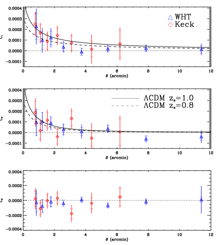
Figure 9: Shear correlation functions compared for the WHT and Keck. The inner error bars correspond to statistical errors only, while the outer error bars correspond to the total errors (statistical + sample variance). For comparison, the correlation functions expected for a $\Lambda$CDM model with $\Omega_{m}=0.3$, $\sigma_{8}=1$ and $\Gamma=0.21$. A median source redshift of $z_{s}$=0.8 and 1.0 are shown, as appropriate for WHT and Keck, respectively.

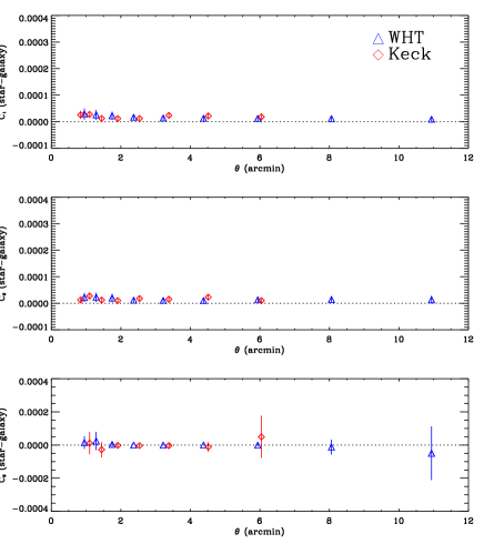
Figure 10: Star-galaxy correlation contribution to the error budget. Demonstrates the negligbly small residual alignment of galaxy shear measurements to the orientation of the original PSF (note the same scale on the $y$-axis as figure 9 above).

We can use the formalism of section 5.1 to evaluate the systematic contribution of residual stellar anisotropy to our shear correlation function. For this purpose, we measure the star-galaxy correlation function given by equation (11) for all of our WHT fields, and show the results on Figure 10. Note that, bearing in mind that the scale on this figure is the same as for our shear correlation function, the systematic contribution due to our anisotropy correction is entirely negligible; it is lower than the shear signal by a factor $>10$ everywhere.

6.2 Sources of Error and Covariance between Angular Scales

It is instructive to compare the different sources of error for each telescope, given the complementary survey strategies. Figure 11 shows the error variance of the shear correlation correlation functions $C_{1}+C_{2}$ of Figure 9 as a function of angular scale $\theta$. The total error variance (from Eq. [7]) was decomposed into a statistical error (from Eq. [9]) and a sample variance contribution (computed by subtracting the latter from the former). The cosmic variance contribution is clearly significant for both Keck and WHT and must be taken into account in the determination of cosmological parameters from cosmic shear data.

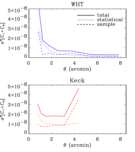
Figure 11: Errors in the shear correlation correlation function $C_{1}+C_{2}$ as a function of angular scale $\theta$ for both WHT (top) and Keck (bottom). The total error variance (solid line) is decomposed into a statistical (dotted line) and a sample variance (dashed line) contribution in each case. Note that the area of the WHT survey is a factor of about 1.7 larger than that for Keck.

The advantage of using a 10m-class telescope in reducing statistical errors is apparent in this Figure. Indeed, the statistical errors for Keck for $\theta\la 3^{\prime}$ are significantly smaller than that for WHT, after scaling them down by a factor of 1.7 corresponding to a common survey area of 1 deg² in both surveys. The much shorter exposure times allowed by Keck yield an improvement in the seeing, tracking errors and overall image quality. Aided by the finer pixellisation of the ESI CCD, this results in an increased galaxy number density and correspondingly lower statistical errors when normalised by survey area (as predicted by Bacon et al 2001). Of course, the statistical errors for WHT are smaller on large angular scales ($\theta\ga 3^{\prime}$) thanks to the larger field of view of this telescope.

The covariance of the shear correlation functions on different angular scales is also non-negligible. Figures 12 and 13 show the covariance matrix for the $C_{1}$ correlation function for WHT and Keck, respectively. In each case, the angular bins correspond to the $\theta$ values shown in Figure 9. The WHT correlation function clearly has important covariance between bins on small angular scales ($\theta\la 3^{\prime}$). The Keck correlation functions also has important covariance on large scales ($\theta\ga 3^{\prime}$). This is due to the elongated field geometry of the Keck camera. In both cases, it is important to include the full covariance matrix for the determination of cosmological parameters.

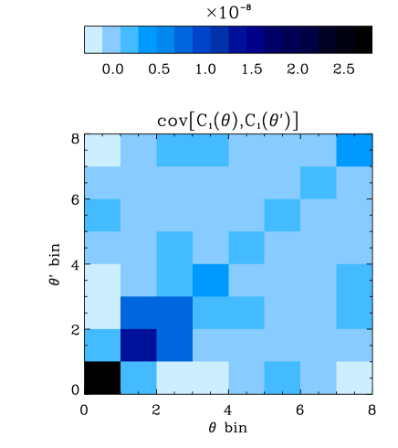
Figure 12: Covariance matrix of the shear $C_{1}$ correlation function between the different angular bins of the WHT data plotted in figure 9.

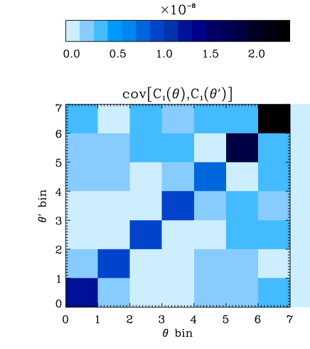
Figure 13: Covariance matrix of the shear $C_{1}$ correlation function between the different angular bins of the Keck data plotted in figure 9.

6.3 Shear Variance

We now wish to compare our results to those obtained recently by other groups. Since many of these results are quoted in terms of the angular dependence of the shear variance, we use equation (13) to convert our correlation function measurements into shear variance measures as a function of scale.

The results for the WHT and Keck surveys, are plotted in Figure 14. Taking the most significant point in each case and using statistical errors only, we find that the cosmic shear signal is detected at the $3.7\sigma$, $3.5\sigma$ and $5.1\sigma$ level with Keck, WHT, and both combined, respectively. Also plotted are the predictions for the $\Lambda$CDM model with $\Omega_{m}=0.3$ and $\Gamma=0.21$ as before. They are shown for a range of values of the galaxy median redshift $z_{s}$, corresponding roughly to the uncertainty and survey-to-survey variations in this parameter. Both old ($\sigma_{8}=1$) and new cluster normalisations ($\sigma_{8}=0.7$) are shown (see discussion below). We also plotted the measurements from other groups, namely from van Waerbeke et al 2000 (CFHT vW+), Kaiser et al. 2000 (CFHT K+), Wittman et al 2000 (CTIO), Maoli et al 2001 (VLT), and van Waerbeke et al 2001 (CFHT vW++). Note that the errors for the VLT, CFHT vW+ and CFHT vW++ do not include cosmic variance. All of the above groups are obtaining results which are broadly consistent with each other and with $\Lambda$CDM with the older normalisation of $\sigma_{8}=1$.

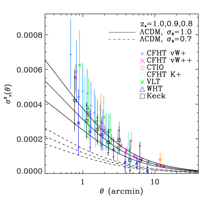
Figure 14: Shear variance as a function of aperture radius. Our measurements with Keck and WHT are shown along with those of other groups (see text). Again, the inner and outer error bars correspond to statistical and total uncertainties, respectively. The expected shear variances for a $\Lambda$CDM model with $\Omega_{m}=0.3$, and $\Gamma=0.21$ are also shown for a range of values for the median source redshift $z_{s}$ corresponding approximately to the uncertainty in this parameter. The models are shown both for $\sigma_{8}\simeq 1$ (solid lines) and $\sigma_{8}\simeq 0.7$ (dashed) cluster normalisation.

6.4 Cosmological Constraints

Now that we have measurements of cosmic shear on several scales, we can determine the implications for cosmological parameters. In order to do this, we use a Maximum Likelihood approach. We first construct data vectors ${\mathbf{d}}\equiv\{C_{1}(\theta_{n}),C_{2}(\theta_{n})\}$ which are simply a rearrangement of our observed correlation functions. We consider a $\Lambda$CDM model with two parameters, $a_{1}=\Omega_{m}$ and $a_{2}=\sigma_{8}$. The shape parameter $\Gamma$ for the matter power spectrum is set to 0.21 as indicated by recent measurements of galaxy clustering (Percival et al. 2001; Szalay et al. 2001). Using the formalism described in BRE and in section 5, we can compute the correlation function for any values of these parameters and arrange them as a theory vector ${\mathbf{t}}({\mathbf{a}})$ set out in exactly the same form as our data vector. The median redshift $z_{s}$ is set to 0.8 and 1.0 for WHT and Keck respectively.

Because the correlation functions were derived from an average over a large number of fields, the central limit theorem ensures that our errors (and covariances) are gaussian. In this case the log-likelihood is simply

$$\chi^{2}=[{\mathbf{d}}-{\mathbf{t}}(a)]^{T}{\mathbf{V}}^{-1}[{\mathbf{d}}-{\mathbf{t}}(a)],$$ (15)

where ${\mathbf{V}}$ is the covariance matrix computed using Equation (8). We minimise this quantity as a function of ${\mathbf{a}}$ to find the best estimate of the normalisation of the power spectrum. To compute confidence contours, we numerically integrate the probability distribution function $P({\mathbf{a}})\propto e^{-\chi^{2}/2}$.

The constraints for our Keck and WHT data, taken separately, are shown on figures 15 and 16. Note that they do not include the uncertainty in $z_{s}$ and in the shear measurement method. These two sources of errors will be included in our final estimate below. The constraints from each of the data set are consistent with each other. As is apparent on the figures, the constraints reveal the well known degeneracy between $\sigma_{8}$ and $\Omega_{m}$ when 2-point statistics alone are used. The wider angular range of WHT allow us to start breaking this degeneracy, by rejecting large values of $\Omega_{m}$ (see van Waerbeke et al. 2001). Note that the width of the contours for Keck and WHT are comparable, even though the WHT area is larger by about 70%. This results from the larger number density of galaxies afforded by Keck thanks to the better seeing statistics and smaller pixel size (see discussion in Bacon et al. 2001).

Figure 15: Constraints on the joint distribution of $\Omega_{m}$ and $\sigma_{8}$ from our Keck measurement. The solid contours correspond to 68% and 95% confidence levels. Note that these contours include statistical errors and non-gaussian sample variance, but do not include the uncertainty in the galaxy redshifts and in the shear measurement method. Also shown are the $1\sigma$ contours from the old (Pierpaoli et al. 2001) and new (Seljak 2001) cluster abundance normalisation.

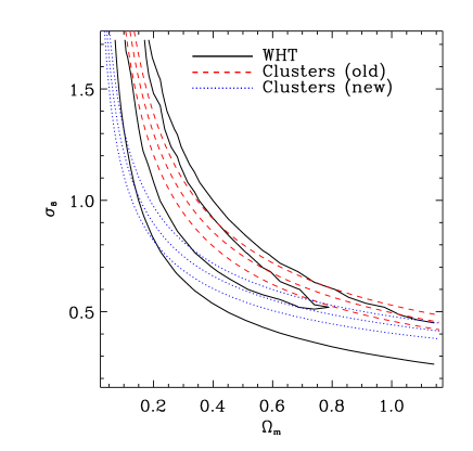
Figure 16: Constraints on the joint distribution of $\Omega_{m}$ and $\sigma_{8}$ as in the previous figure, but for our WHT measurement.

The constraints on $\sigma_{8}$ and $\Omega_{m}$ obtained by combining the Keck and WHT data are shown in Figure 17. As expected, the combined contours are consistent with the two measurements taken separately. A good fit to our 68% confidence level is given by

$$\sigma_{8}\left(\frac{\Omega_{m}}{0.3}\right)^{0.68}=0.97^{+0.10}_{-0.09}~{}~{}~{}~{}{\rm(shot\ noise+sample\ variance)}$$ (16)

with $0.14<\Omega_{m}<0.65$. To this statistical error (which includes non-gaussian sample variance), we also must add that arising from the uncertainty the in the redshift distribution and in the method calibration. A good estimate for these uncertainties can be obtained by noting that the shear variance on the central scale for our experiments, i.e. circular radius of 3 arcmins, scales as $\sigma^{2}_{\gamma}\propto P_{\gamma}^{-2}\sigma_{8}^{2.5}z_{s}^{1.6}$, where $P_{\gamma}^{-1}$ is the ellipticity-to-shear conversion factor in the KSB method (see BRE). This factor was shown to have a $1\sigma$ uncertainty of 5% (BRE). The uncertainty in $z_{s}$ is about 12% for our two data sets (see §3 and §4). Using the former expression to propagate the errors yields a final constraint on the amplitude of the matter power spectrum of $\sigma_{8}(\Omega_{m}/0.3)^{0.68}=0.97^{+0.10}_{-0.09}\pm 0.07\pm 0.04$, where the error bars denote 68% confidence levels, arising from statistical (incl. sample variance), redshift uncertainty and $P_{\gamma}$ uncertainty, respectively. Adding these errors in quadrature, we obtain our final estimate for the amplitude of the power spectrum, namely

$$\sigma_{8}\left(\frac{\Omega_{m}}{0.3}\right)^{0.68}=0.97\pm 0.13~{}~{}~{}{\rm(total~{}error)},$$ (17)

where the error is the total error for a 68% confidence level.

Figure 17: Constraints on the joint distribution of $\Omega_{m}$ and $\sigma_{8}$ for the combination of our Keck and WHT measurements.

Our results are consistent with the results of van Waerbeke et al. (2002) who found $\sigma_{8}=(0.94\pm 0.07)(\Omega_{m}/0.3)^{0.24^{-0.18}_{+0.18}\Omega_{m}-0.49}$ (68%CL), after marginalising over $\Gamma$ in the range 0.1 to 0.4. They are also consistent with those of Hoekstra et al. (2002) who found $\sigma_{8}=0.81^{+0.14}_{-0.19}$ (95%CL) for $\Omega_{m}=0.3$ and $\Gamma=0.21$.

It is interesting to compare our measurement of $\sigma_{8}$ to that derived from cluster abundance. Our results are in agreement with the older normalisation of the power spectrum from cluster abundance. Until recently, the cluster abundance was indeed quoted to be $\sigma_{8}=(1.00\pm 0.07)(0.3/\Omega_{m})^{0.60}(\Gamma/0.21)^{0.28-0.31\Omega_{m}}$ ($1\sigma$; Pierpaoli et al. 2001; see also earlier and consistent estimates by Eke et al. 1998; Viana and Liddle 1999). Recently the cluster normalisation has been revised to a lower value, mainly because of the use of the observed mass-temperature relation for clusters, rather than the simulated one. For instance, Seljak (2001) finds $\sigma_{8}=(0.75\pm 0.06)(0.3/\Omega_{m})^{0.44}(\Gamma/0.21)^{0.08}$ ($1\sigma$; see also Borgani et al 2001; Rieprich & Böhringer 2001; Viana et al. 2001). A similar normalisation was found by combining the 2dF galaxy survey with CMB measurements by Lahav et al. (2001). The two cluster normalisations are also plotted on Figures 15, 16 and 17. Clearly our results are most consistent with a $\sigma_{8}=1$ normalisation, but do not rule out the new normalisation which is consistent at the 1.7$\sigma$ level for $\Omega_{m}=0.3$. This can also be seen by examining Figure 14 which shows the impact of these different normalisations for the shear variance.

7 Conclusions

We have presented a thorough analysis of weak lensing signals obtained using two telescopes. The independent instruments introduce different systematic effects upon galaxy shapes, the cross-checking and control of which is the most important challenge facing current measurements of weak shear. Our many-line-of-sight survey strategy for cosmic shear, using 173 Keck telescope fields, also complements an alternative 20 large-field survey strategy with the William Herschel Telescope.

We have measured cosmic shear at a signal-to-noise of 5.1$\sigma$ with both Keck and WHT, and have measured the amplitude of the power spectrum, $\sigma_{8}\left(\frac{\Omega_{m}}{0.3}\right)^{0.68}=0.97\pm 0.13$ with $0.14<\Omega_{m}<0.65$, including all contributions to the 68% CL uncertainty: statistical noise, sample variance, covariance between angular bins, systematic effects, and redshift uncertainty. A measurement of this quantity from cosmic shear is cosmologically valuable, as it represents a direct measure of the amplitude of mass fluctuations.

These measurements have been obtained after a careful study and removal of systematic effects which can mimic a shear signal at the 1% level. We have demonstrated for both telescopes that no offset in the ensemble of shear estimators is found as a function of position on images, and that the contribution of star-galaxy correlations is negligible with our catalogue selection. Our methods have been tested thoroughly in the context of detailed simulations of realistic images (Bacon et al. 2001) and have been shown to operate successfully in recovering shear at the necessary level.

Our results for Keck and WHT are consistent with each other, strengthening confidence in control of systematics. The joint results are also consistent with other recent cosmic shear measurements (Hoekstra et al. 2002; van Waerbeke et al. 2002). They also agree with the old cluster abundance normalisation (Eke et al. 1998; Viana and Liddle 1999; Pierpaoli et al. 2001). Our results prefer this normalisation, but can not rule out lower cluster-abundance normalisation which has recently been derived (Borgani et al 2001; Seljak 2001; Rieprich & Böhringer 200; Viana et al. 2001; see also the similar normalisation derived from 2dF+CMB by Lahav et al. 2001). This discrepancy, if confirmed, could arise from unknown systematics in either the cluster or cosmic shear methods. Note for instance that uncorrected systematics in cosmic shear measurements will tend to add to the lensing signal and thus lead to an overestimation of $\sigma_{8}$. For the cluster method, further studies would be needed to understand the difference between the observed mass-temperature relation and that found in numerical simulations. It is important to understand the origin of the discrepancy between cosmic shear and cluster abundance methods. If this is not explained by such systematics, it could point towards a failure of the standard $\Lambda$CDM paradigm, and therefore have important consequences for cosmology.

References

- [1] Bacon D. J., Refregier A. R., Ellis R. S., 2000, MNRAS, 318, 625 (BRE)
- [2] Bacon D. J., Refregier A., Clowe D., Ellis R. S., 2001, MNRAS, 325, 1065
- [3] Bartelmann M., Schneider P., 2000, Physics Reports, 340, 291
- [4] Baugh C. M., Cole S., Frenk C. S., Lacey C. G., 1998, ApJ, 498, 504
- [5] Bernardeau F., van Waerbeke L., Mellier Y., 1997, A&A, 322, 1
- [6] Bertin E., Arnouts S., 1996, A&AS, 117, 393
- [7] Bernardeau, F., van Waerbeke, L., & Mellier, Y., 1997, A&A, 322, 1
- [8] Blandford R. D., Saust A. B., Brainerd T. G., Villumsen J. V., 1991, MNRAS, 251, 600
- [9] Borgani S., Rosati P., Tozzi P., Stanford S. A., Eisenhardt P. R., Lidman C., Holden B., Della Ceca R., Norman C., Squires G., 2001, ApJ, 561, 13.
- [10] Brown M. L., Taylor A. N., Hambly N. C., Dye S., 2000, astro-ph/0009499
- [11] Carter D., Bridges T., 1995, WHT Prime Focus and Auxiliary Port Imaging Manual, available at http:/lpss1.ing.iac.es/manuals/html_manuals/wht_instr/pfip
- [12] Catelan P., Kamionkowski M., Blandford R. D., 2001, MNRAS, 320, L7
- [13] Cohen J. G., Hogg D. W., Blandford R., Cowie L. L., Hu E., Songaila A., Shopbell P., Richberg K., 2000, ApJ, 538, 29
- [14] Crittenden R. G., Natarajan P., Pen U.-L., Theuns T., 2000, astro-ph/0012336
- [15] Croft R. A. C., Metzler C. A., 2000, ApJ, 545, 561
- [16] Eke V. R., Cole S., Frenk C., Henry H. J., 1998, MNRAS, 298, 1145
- [17] Erben T., van Waerbeke L., Bertin E., Mellier Y., Schneider P., 2001, A&A, 366, 717
- [18] Hämmerle et al., 2001, submitted to A&A, preprint astro-ph/0110210
- [19] Heavens A., Refregier A., Heymans C., 2000, MNRAS, 319, 649
- [20] Hoekstra H., Franx M., Kuijken K., Squires G., 1998, ApJ, 504, 636
- [21] Hoekstra H., Yee, H.K.C., Gladders, M.D., Felipe Barrientos, L., Hall, P.B., & Infante, L., 2002, submitted to ApJ, preprint astro-ph/0202285
- [22] Jain B., Seljak U., 1997, ApJ, 484, 560
- [23] Jain B., Seljak U., White S., 2000, ApJ, 530, 547
- [24] Kaiser N., 1992, ApJ, 388, 272
- [25] Kaiser N., Squires G., Broadhurst T., 1995, ApJ, 449, 460
- [26] Kaiser N., 1998, ApJ, 498, 26
- [27] Kaiser N., Wilson G., Luppino G. A., 2000, astro-ph/0003338
- [28] Kamionkowski M., Babul A., Cress C. M., Refregier A., 1998, MNRAS, 301, 1064
- [29] Kauffmann G., Guiderdoni B., White S. D. M., 1994, MNRAS, 267, 981
- [30] Lahav, O., et al. 2001, submitted to MNRAS, astro-ph/0112162
- [31] Luppino G. A., Kaiser N., 1997 , ApJ, 475, 20
- [32] Lupton R., 1993, Statistics in Theory and Practice (Princeton U. Press: Princeton)
- [33] Maoli R., van Waebeke L., Mellier Y., Schneider P., Jain B., Bernardeau F., Erben T., Fort B., 2001, A&A, 368, 766
- [34] Massey R., Bacon D., Refregier A., Ellis R., to appear in A New Era In Cosmology, eds. T. Shanks & N. Metcalfe, ASP Conference Series, preprint astro-ph/0112393
- [35] Mould J., Blandford R., Villumsen J., Brainerd T., Smail I., Smail I., Small T., Kells W., 1994, MNRAS, 271, 31
- [36] Pierpaoli E., Scott D., White M., 2001, MNRAS, 325, 77
- [37] Percival W. et al., 2001, MNRAS, 327, 1297
- [38] Reiprich T.H. & Böhringer H., 2001, to appear in ApJ, preprint astro-ph/0111285
- [39] Refregier A., Rhodes, J., Groth E., 2002, submitted to ApJL
- [40] Rhodes J., 1999, PhD thesis, Department of Physics, Princeton University
- [41] Rhodes J., Refregier A., Groth E., 2000, ApJ, 536, 79
- [42] Rhodes J., Refregier A., Groth E., 2001, ApJ, 552, L85
- [43] Seljak U., 2001, submitted to MNRAS, preprint astro-ph/0111362
- [44] Schneider P., Ehlers J., Falco E. E., 1992, Gravitational Lenses, Springer Verlag, Heidelberg
- [45] Szalay A. et al., 2001, preprint astro-ph/0107419
- [46] Van Waerbeke L., Bernardeau F., Mellier Y., 1999, A&A, 342, 15
- [47] Van Waerbeke L., Mellier Y., Erben T., Cuillandre J. C., Bernardeau F., Maoli R., Bertin E., McCracken H. J., Le Fèvre O., Fort B., Dantel-Fort M., Jain B., Schneider P., 2000, A&A, 358, 30
- [48] Van Waerbeke L., Mellier Y., Radovich M., Bertin E., Dantel-Fort M., McCracken H. J., Le Fèvre O., Foucaud S., Cuillandre J.-C., Erben T., Jain B., Schneider P., Bernardeau F., Fort B., 2001, A&A, 374, 757
- [49] Van Waerbeke, L., Mellier, Y., Pelló, R., Pen, U.-L., McCracken, H.J., & Jain, B., 2002, submitted to A&A, preprint astro-ph/0202503
- [50] Viana P., Liddle A., 1999, MNRAS, 303, 535
- [51] Viana P.T.P., Nichol R.C., Liddle A.R., 2001, submitted to ApJL, preprint astro-ph/0111394
- [52] Wittman D. M., Tyson J. A., Kirkman D., Dell’Antonio I., Bernstein G., 2000, Nature, 405, 143