Likelihood Analysis of Cosmic Shear
on Simulated and VIRMOS-DESCART Data

We present a maximum likelihood analysis of cosmological parameters from measurements of the aperture mass up to $35$ arcmin, using simulated and real cosmic shear data. A four-dimensional parameter space is explored which examines the mean density $\Omega_{M}$, the mass power spectrum normalization $\sigma_{8}$, the shape parameter $\Gamma$ and the redshift of the sources $z_{s}$. Constraints on $\Omega_{M}$ and $\sigma_{8}$ (resp. $\Gamma$ and $z_{s}$) are then given by marginalizing over $\Gamma$ and $z_{s}$ (resp. $\Omega_{M}$ and $\sigma_{8}$). For a flat $\Lambda$CDM cosmologies, using a photometric redshift prior for the sources and $\Gamma\in[0.1,0.4]$, we find $\sigma_{8}=\left(0.57\pm 0.04\right)\Omega_{M}^{\left(0.24\mp 0.18\right)\Omega_{M}-0.49}$ at the $68\%$ confidence level (the error budget includes statistical noise, full cosmic variance and residual systematic). The estimate of $\Gamma$, marginalized over $\Omega_{M}\in[0.1,0.4]$, $\sigma_{8}\in[0.7,1.3]$ and $z_{s}$ constrained by photometric redshifts, gives $\Gamma=0.25\pm 0.13$ at $68\%$ confidence. Adopting $h=0.7$, a flat universe, $\Gamma=0.2$ and $\Omega_{m}=0.3$ we find $\sigma_{8}$=0.98 $\pm 0.06$ . Combined with CMB, our results suggest a non-zero cosmological constant and provide tight constraints on $\Omega_{M}$ and $\sigma_{8}$. We finaly compare our results to the cluster abundance ones, and discuss the possible discrepancy with the latest determinations of the cluster method. In particular we point out the actual limitations of the mass power spectrum prediction in the non-linear regime, and the importance for its improvement.

1 Introduction

In the standard cosmological picture, the structures in the Universe grow from the gravitational collapse of initial Gaussian density perturbations. The properties of mass distribution at low redshift are expected to express the latest and one of the most explicit footprint of the formation process, so their description from cosmological surveys can be challenged against theoretical predictions resulting from this paradigm. For example, a direct observation of the mass distribution in structures is believed to be an unequivocal test of cosmological scenario of structure formation. If so, the weak gravitational lensing produced on distant galaxies by large scale structures is a direct probe of dark matter, regardless the light distribution. It is therefore a robust technique to challenge the current cosmological models. In particular, it can reliably probe small angular scale and look into the transition to the quasi-linear and non-linear regimes, where comparison between observations and cosmological models are still difficult.

The cosmological origin of the coherent distortion fields detected in cosmic shear surveys is now firmly established (Bacon et al., 2000; Haemmerle et al., 2001; Hoekstra et al., 2002; Kaiser et al., 2000; Maoli et al., 2001; Pen et al., 2001; Rhodes et al., 2001; Van Waerbeke et al., 2000, 2001b; Wittman et al., 2000). Van Waerbeke et al. (2001b) have shown that the measurements provided by different statistical estimators of distortion signal are consistent with the gravitational lensing hypothesis with a high confidence level, so that present-day data can already constrain cosmological parameters. Their joint estimate of the mass density $\Omega_{M}$ and the power spectrum normalization $\sigma_{8}$ led to consistent results with the cluster abundance constraints (Pierpaoli et al., 2001) and confirmed earlier tentative obtained by Maoli et al. (2001) and Rhodes et al. (2001) using ESO-VLT/CFHT and HST data respectively. A recent measurement done on a shallow survey (therefore very different in depth) confirmed also this agreement (Hoekstra et al., 2001, 2002).

So far, the cosmological parameter estimation from cosmic shear relied on prior knowledge of the slope of the mass power spectrum $\Gamma$ and/or the mean redshift $\bar{z}_{s}$ of the lensed galaxy population. In fact, the statistical properties of cosmic shear depends significantly on these quantities (Kaiser, 1992; Bernardeau et al., 1997; Jain & Seljak, 1997), so any prior on these parameters may have a serious impact on the cosmological parameter estimation. For instance changing the shape of the power spectrum in either direction would favor low or high matter densities, by changing the normalization accordingly. This ambiguity expresses a degeneracy between the normalization and the mass density, which depends on the choice of $\Gamma$ (Van Waerbeke et al., 2001b). Jain & Seljak (1997) addressed this issue by pointing out that a measurement of the cosmic shear in both linear and non-linear scales could break the degeneracy, so that one in principle recover simultaneously $\Gamma$, $\sigma_{8}$ and $\Omega_{M}$ from the shear variance alone. Unfortunately, the redshift of the sources is also a strongly degenerate parameter with $\sigma_{8}$, which definitely hampers shear variance analysis to provide unequivocal discrimination of cosmological models. In fact, stringent constraints on the cosmological parameters from the shear variance are possible only with an accurate knowledge of the source redshifts and a measurement which extends over a large range of scales.

In this paper we carry out a full maximum likelihood analysis of cosmic shear data over the four parameters $\Omega_{M}$, $\sigma_{8}$, $\Gamma$, and $\bar{z}_{s}$ for flat and open cosmologies. Using both simulations and observations, we study slices and projections in this parameter space and discuss the reliability of cosmological constraints which are based on catalogues having similar size and depth as current cosmic shear surveys. In particular we give an estimate of $\Omega_{M}$ and $\sigma_{8}$ by marginalizing over the power spectrum shape and sources redshifts. The improvement of our knowledge of the source redshift is crucial to gain better accuracy for the other parameters. In this work we use photometric redshifts to put priors on the source redshift distribution.

The paper is organized as follows. Section 2 presents a brief summary of some theoretical concepts and introduces the shear estimators used throughout the paper. Section 3 describes the data and how shear quantities were obtained from the survey catalogue. The likelihood method and the details of the priors are presented in Section 4. Section 5 shows and discusses the results on the parameter estimates on both simulated and real surveys. Finally, conclusions are presented in Section 6.

2 Theory

Following the notation in Schneider et al. (1998), we define the power spectrum of the convergence as

$$P_{\kappa}(k) = {9\over 4}\Omega_{0}^{2}\int_{0}^{w_{H}}{{\rm d}w\over a^{2}(w)}P_{3D}\left({k\over f_{K}(w)};w\right)\times$$ (1)

$$\left[\int_{w}^{w_{H}}{\rm d}w^{\prime}n(w^{\prime}){f_{K}(w^{\prime}-w)\over f_{K}(w^{\prime})}\right]^{2},$$

where $f_{K}(w)$ is the comoving angular diameter distance out to a distance $w$ ($w_{H}$ is the horizon distance), and $n(w(z))$ is the redshift distribution of the sources given in Eq.(12). $P_{3D}(k)$ is the non-linear mass power spectrum computed according to Peacock & Dodds (1996), and $k$ is the 2-dimensional wave vector perpendicular to the line-of-sight. The top-hat shear variance (smoothing window of radius $\theta_{c}$) and the shear correlation function can be written as

$$\langle\gamma^{2}\rangle={2\over\pi\theta_{c}^{2}}\int_{0}^{\infty}\leavevmode\nobreak\ {{\rm d}k\over k}P_{\kappa}(k)[J_{1}(k\theta_{c})]^{2},$$ (2)

$$\langle\gamma\gamma\rangle_{\theta}={1\over 2\pi}\int_{0}^{\infty}\leavevmode\nobreak\ {\rm d}k\leavevmode\nobreak\ kP_{\kappa}(k)J_{0}(k\theta).$$ (3)

Because the weak distortion field can be generated by non-lensing mechanisms, it is important to measure separately the $E$ and $B$ components of the shear. These modes were introduced initially to test for the gravitational origin of the lensing signal (Crittenden et al., 2000) since a potential gravitational field is expected to produce only curl-free shear patterns ($E$ mode). Any measurable $B$ mode should be interpreted as a measurement of residual systematic in the data (Point Spread Function correction, intrinsic alignment or anything else) and must be removed from the weak lensing signal prior to cosmological interpretation of cosmic shear data.

The extraction of both modes is not trivial. The $E$ and $B$-modes decompositions of the top-hat shear variance, and of the shear correlation function given in Eq.(2,3) are only defined up to a integration constant (see Crittenden et al., 2000; Pen et al., 2001). This constant depends on the extrapolated cosmic shear signal either at small ($<30$ arc-seconds) or large ($>1$ degree) scales. These boundary conditions turn out to be a severe limitation which hampers reliable derivations of both modes from our present-day data because we do not cover yet very large angular scales and we still suffer from systematics on very small scales which are not well understood. As pointed out by Pen et al. (2001), the only unambiguous $E$ and $B$ mode decomposition is carried out by the aperture mass, $M_{ap}$:

$$M_{\rm ap}=\int_{\theta<\theta_{c}}\leavevmode\nobreak\ {\rm d}^{2}{{\hbox{$\bf\theta$}}}\kappa({{\hbox{$\bf\theta$}}})\leavevmode\nobreak\ U(\theta),$$ (4)

where $\kappa({{\hbox{$\bf\theta$}}})$ is the convergence field, and $U(\theta)$ is the zero mass aperture window (Schneider et al., 1998):

$$U(\theta)={9\over\pi\theta_{c}^{2}}\left(1-{\theta^{2}\over\theta_{c}^{2}}\right)\left({1\over 3}-{\theta^{2}\over\theta_{c}^{2}}\right).$$ (5)

This estimator was introduced in Kaiser et al. (1994) to study clusters of galaxies, but it also has an important potential for cosmic shear analysis (Schneider et al., 1998).

$\langle M_{\rm ap}^{2}\rangle$ can be calculated directly from the shear $\bf\gamma$ without the need for a mass reconstruction. It can be rewritten as a function of the shear if we express ${{\hbox{$\bf\gamma$}}}=(\gamma_{t},\gamma_{r})$ in the local frame of the line connecting the aperture center to the galaxy. $M_{\rm ap}$ can therefore be expressed as function of $\gamma_{t}$ only (Miralda-Escude, 1991; Kaiser, 1992):

$$M_{\rm ap}=\int_{\theta<\theta_{c}}\leavevmode\nobreak\ {\rm d}^{2}{{\hbox{$\bf\theta$}}}\gamma_{t}({{\hbox{$\bf\theta$}}})\leavevmode\nobreak\ Q(\theta),$$ (6)

where the filter $Q(\theta)$ is given from $U(\theta)$:

$$Q(\theta)={2\over\theta^{2}}\int_{0}^{\theta}\leavevmode\nobreak\ {\rm d}\theta^{\prime}\leavevmode\nobreak\ \theta^{\prime}\leavevmode\nobreak\ U(\theta^{\prime})-U(\theta)$$ (7)

The aperture mass variance is related to the convergence power spectrum (Eq.1)by:

$$\langle M_{\rm ap}^{2}\rangle={288\over\pi\theta_{c}^{4}}\int_{0}^{\infty}\leavevmode\nobreak\ {{\rm d}k\over k^{3}}P_{\kappa}(k)[J_{4}(k\theta_{c})]^{2}.$$ (8)

The $B$-mode is obtained by replacing $\gamma_{t}$ with $\gamma_{r}$ in Eq.(6). Although this estimator is robust and does not depend on an unknown integration constant, it is less sensitive to cosmological parameters than the top-hat variance or the shear correlation functions (Van Waerbeke et al., 2001b).

3 Measurements

We use the observations done within the VIRMOS-DESCART project by the VIRMOS imaging and spectroscopic survey. The data cover an effective area of 8.5 sq.deg. in the I-band, with a limiting magnitude $m_{I_{AB}}=24.5$. Technical details of the data set are given in Van Waerbeke et al. (2001b). We applied a bright magnitude cut at $m_{I}=21$ in order to exclude the foreground objects from the source galaxies. The shape of the galaxies are measured and analyzed as described in this paper, to which we refer for technical details.

The location of the $i$-th galaxy is given by ${{\hbox{$\bf\theta$}}}_{i}$, the ellipticity by ${\bf e}({{\hbox{$\bf\theta$}}}_{i})=(e_{1},e_{2})$, and its weight $w_{i}$. The ellipticity is an unbiased estimate of the shear ${{\hbox{$\bf\gamma$}}}({{\hbox{$\bf\theta$}}}_{i})$. The quantity measured on the data are the binned tangential and radial shear correlation functions. They are given by a sum over galaxy pairs $({{\hbox{$\bf\theta$}}}_{i},{{\hbox{$\bf\theta$}}}_{j})$

$$\xi_{tt}(r) = {\displaystyle\sum_{i,j}w_{i}w_{j}e_{t}({{\hbox{$\bf\theta$}}}_{i})\cdot e_{t}({{\hbox{$\bf\theta$}}}_{j})\over\displaystyle\sum_{i,j}w_{i}w_{j}}$$

$$\xi_{rr}(r) = {\displaystyle\sum_{i,j}w_{i}w_{j}e_{r}({{\hbox{$\bf\theta$}}}_{i})\cdot e_{r}({{\hbox{$\bf\theta$}}}_{j})\over\displaystyle\sum_{i,j}w_{i}w_{j}},$$ (9)

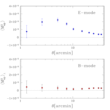
Figure 1: Above is the aperture mass statistic $\langle M_{\rm ap}^{2}\rangle$ ($E$-mode) and below the aperture mass $\langle M_{\rm ap}^{2}\rangle_{\perp}$ computed with galaxies rotated by $45$ degrees ($B$-mode). Error bars are $1-\sigma$ statistical errors.

where $r=|{{\hbox{$\bf\theta$}}}_{i}-{{\hbox{$\bf\theta$}}}_{j}|$, and $(e_{t},e_{r})$ are the tangential and radial ellipticities defined in the frame of the line connecting a pair of galaxies.

From Eq.(9), we define $\xi_{+}(r)$ and $\xi_{-}(r)$ which are respectively the sum and the difference of the two correlation functions:

$$\xi_{+}(r)=\xi_{tt}(r)+\xi_{rr}(r);\ \ \xi_{-}(r)=\xi_{tt}(r)-\xi_{rr}(r).$$ (10)

Both $\xi_{+}(r)$ and $\xi_{-}(r)$ are computed from a summation of the correlation function defined in Eq.(10), while the $E$ and $B$ modes aperture mass are derived by integration of the correlation functions with an appropriate window (see Crittenden et al. (2000) for general derivations and Pen et al. (2001) for a practical application to our filter).

The $E$ mode aperture mass is

$$\langle M_{\rm ap}^{2}\rangle=\pi\int_{0}^{2\theta_{c}}rdr{\cal W}(r)\xi_{+}(r)+\pi\int_{0}^{2\theta_{c}}rdr\tilde{\cal W}(r)\xi_{-}(r),$$ (11)

where ${\cal W}(r)$ and $\tilde{\cal W}(r)$ are given in Crittenden et al. (2000). The $B$-mode is obtained by changing the sign of the second term in Eq.(11) (which is equivalent to the $45$ degrees rotation test, or else $\gamma_{t}\rightarrow\gamma_{r}$).

Figure 1 shows the $E$ mode (top) and $B$ mode (bottom) measured in our galaxy sample. Using the $B$-mode measurement, we found the source of the residual systematics at $3-4^{\prime}$ reported by Van Waerbeke et al. (2001b) and Pen et al. (2001): it was caused by the third order polynomial fit to the PSF, which produced wings at the edge of the CCDs. A second order fitting removed most of the unwanted $B$ mode contribution without spoiling the $E$ mode signal. As shown in Figure 1, the residual systematics are consistent with zero up to 10 arc-minutes and remains flat over the whole angular scale explored by the data. Clearly, the signal is dominated by the $E$ mode contribution at least up to 25 arc-minutes. This demonstrates that signal produced by intrinsic alignment of galaxies is not detected at this level.

4 Parameter Estimation

4.1 Redshift distribution of galaxies in the VIRMOS-DESCART data

We estimated the redshift distribution of our catalogue from a combination of the Hubble Deep Fields North and South data (Fernández-Soto et al., 1999; Chen et al., 1998) and VLT observations of the cluster MS1008-1224. Both HDF and MS1008-1224 observations are much deeper than the cosmic shear sample of galaxies considered in this work, so that magnitude measurements and photometric redshift estimates up to $I_{AB}=24.5$ are based on reliable data with high signal-to-noise ratio.

The VLT MS1008-1224 galaxy sample comprises deep $UBVRI$ observations, carried out by the Science Verification Team (SVT) at ESO/VLT with the FORS1 and FORS2 instruments (Appenzeller et al., 1998) and deep $J$ and $K$ data obtained at the ESO/NTT with SOFI (Program 66.A-0316(A); PI Mellier). The extension of early deep SVT observations to U band with FORS2 and more recently to near infrared with SOFI, which has similar field of view as FORS (5.5 arc-minutes against 6.8 arc-minutes), allow us to considerably improve the accuracy of photometric-redshifts of foreground, cluster and background galaxies over the whole field. As compared to HDF the VLT/NTT observations are not as deep, but they provide a much larger sample of galaxies because they cover of field of view 15 times larger than HDF. In total, 920 galaxies having $I_{AB}\leq 24.5$ and $UBVRIJK$ data have been added to HDF data.

The deep $UBVRI$ data are described at the ESO site and in Athreya et al. (2002). A complete description of the new $J$ and $K$ band data will be presented elsewhere (Gavazzi & et al., 2002). In brief, the exposure times of NTT/SOFI $J$ and $K$ bands were 5h30 and 6h respectively. The completeness limits are $J=23.$ and $K=22.$ and both $J$ and $K$ complete samples encompasses more than 90% of the $I_{AB}\leq 24.5$ galaxies. Hence, most galaxies used for determining the photo-$z$ distribution of galaxies up to $I_{AB}\leq 24.5$ have reliable $J$ and $K$ photometric measurements to secure a collection of redshift on a very large sample of galaxies, which covers a broad magnitude range homogeneously spread over the whole field. The presence of the lensing cluster ($z=0.306$) in the field only affects the redshift range $0.26<z<0.36$. These data have been removed from the sample and the redshift distribution interpolated in this redshift range. The magnification bias may also change the redshift distribution of galaxies inside the very center of the cluster where the gravitational depletion is significant (see Athreya et al., 2002). We therefore also removed the central part ($R<40$ arc-second) of the cluster from the sample. Since this region is also the most contaminated by the brightest cluster members, the depletion itself turns out to have no impact of the galaxy selection criterion.

The photometric redshifts ($z_{phot}$) were measured using the fitting algorithm $hyperz$ developed by Bolzonella et al. (2000). Each $z_{phot}$ is inferred by comparing the spectral energy distribution of galaxies, as sampled by their $UBVRIJK$ photometric flux, to a set of spectral templates representative of common late and early type galaxies which are followed with look-back time according to Bruzual & Charlot’s evolution models (GISSEL98; Bruzual & Charlot, 1993). The validation of $hyperz$ is discussed at length in Bolzonella et al. (2000). It has been conclusively gauged against spectroscopic redshift on MS1008-1224 data by Athreya et al. (2002). Details on photometric redshift techniques can be found in those papers.

The compiled photometric distribution is shown on Fig.2. For the purpose of marginalization we parameterize this distribution with the following normalized function:

$$n(z)={\beta\over z_{s}\ \Gamma\left({1+\alpha\over\beta}\right)}\left({z\over z_{s}}\right)^{\alpha}\exp\left[-\left({z\over z_{s}}\right)^{\beta}\right],$$ (12)

where $\alpha=2$ and $\beta=1.2$. For these values of $\alpha$ and $\beta$, the mean redshift is $\bar{z}_{s}\approx 2.1\ z_{s}$ and the median redshift is $\approx 1.9\ z_{s}$. We allowed $z_{s}$ to vary from $0.24$ to $0.64$, which corresponds to a mean redshift varying from $0.5$ to $1.32$. These two extreme models are shown on Fig.2: they are clearly conservative bounds on the redshift distribution in the data. The curve on Fig.2 shows the best fit model, with $z_{s}=0.44$ ($\bar{z}_{s}=0.9$).

Figure 2: The histogram shows the photometric redshift distribution from the joint VLT and HDF fields. The thick solid line is the theoretical $n(z)$ from Eq.(12) with $z_{s}=0.44$. The low and high redshift thin solid lines correspond to $z_{s}=0.24$ and $z_{s}=0.64$, our extreme redshift distributions used in this paper.

4.2 Maximum Likelihood

The dominant cosmological parameters for the 2-point cosmic shear statistics are the mean mass density $\Omega_{M}$, the power spectrum normalization $\sigma_{8}$, the shape parameter $\Gamma$ and the redshift of the sources (see Bernardeau et al., 1997; Jain & Seljak, 1997; van Waerbeke et al., 1999) Our parameter space has therefore four dimensions, but we truncate the exploration volume inside a realistic range defined as $\Omega_{M}\in[0.1,1]$, $\sigma_{8}\in[0.3,1.6]$ and $\Gamma\in[0.05,0.7]$ with a sampling of $10\times 14\times 14$. For the analysis of the VIRMOS-DESCART data, the redshift of sources is parameterized by Eq.(12) with $z_{s}\in[0.24,0.64]$ and a sampling of $9$. For the simulations, the sources are placed at redshift unity, therefore in the maximum likelihood analysis we assumed we knew the shape (Dirac distribution), but we allowed the redshift $z_{s}$ to vary between $0.7$ and $1.2$ (sampling of $6$). In fact we found that the real shape of the source distribution does not matter, but the agreement with the mean redshift does. This parameter range box ($\Omega_{M}$, $\Gamma$, $\sigma_{8}$, $z_{s}$) defines what we call the default prior box. The model predictions are then interpolated with an oversampling seven times better in each dimension.

Let $d_{i}$ be the data vector (i.e. the aperture mass $\langle M_{\rm ap}^{2}\rangle$ for different scales $\theta_{i}$), and $m_{i}(\Omega_{M},\sigma_{8},\Gamma,z_{s})$ the model predictions. The likelihood function of the data is

$${\cal L}={1\over(2\pi)^{n}|{\bf C}|^{1/2}}\exp\left[(d_{i}-m_{i}){\bf C}^{-1}(d_{i}-m_{i})^{T}\right],$$ (13)

where $n=10$ is the number of scales and ${\bf C}$ is the $10\times 10$ covariance matrix,

$$C_{ij}=\langle(d_{i}-m_{i})^{T}(d_{j}-m_{j})\rangle.$$ (14)

${\bf C}$ can be decomposed as ${\bf C}={\bf C}_{n}+{\bf C}_{s}+{\bf C}_{b}$, where ${\bf C}_{n}$ is the statistical noise, ${\bf C}_{s}$ the cosmic variance covariance matrix and ${\bf C}_{b}$ the residual bias. ${\bf C}_{n}$ has been measured in Pen et al. (2001), so we just reproduce here its general behavior: the top panel on figure 3 shows the cross-correlation coefficient for $2$, $10$, and $35$ arc-min with the other scales.

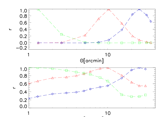
Figure 3: Cross-correlation coefficient between three measurement scales for the statistical noise (above) and the cosmic variance (below). The three scales are $1.3^{\prime}$ (squares), $10.3^{\prime}$ (triangles) and $25.1^{\prime}$ (diamonds). The cosmic variance cross-correlation is obtained from ray-tracing simulations (Jain et al. (2000)).

In order to account for residual systematics, we decided to add quadratically the residual $B$ mode (see the bottom panel in Figure 1) to the error of the signal. Given that there is no clearly identified scheme to deal with the residual systematics yet, this appears to be the safest and most conservative attitude. The diagonal part of the bias correlation matrix ${\bf C}_{b}$ is therefore given by the $B$ mode signal, and the off-diagonal terms follow the same correlation properties as the $E$ mode (the $E$ and $B$ covariance matrices for the statistical noise are actually identical).
The cosmic variance covariance matrix ${\bf C}_{s}$ is trickier to estimate. Assuming the field is Gaussian is too simplistic, since the observed scales are within the non-linear and weakly non-linear regimes, so in principle a complete description of non-Gaussian contributions to the error budget cannot be carried out without detailed cosmological simulations. In order to avoid this heavy procedure, we focused instead on a simpler alternative based on non-linear perturbation theory. It was pointed out in Scoccimarro et al. (1999) that, for the convergence power spectrum, the ratio of the Gaussian to Non-Gaussian errors is almost independent of scale, and close to $1$ for any cosmology. We investigated whether this statement could be also valid in real space, using three ray-tracing simulations for three different cosmological models (Jain et al., 2000).

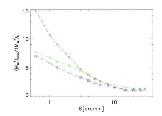
Figure 4: Ratio between the aperture mass dispersion obtained from ray-tracing simulations (Jain et al. (2000)) and the dispersion obtained from the Gaussian field hypothesis for a survey of similar size. The three curves correspond to a $\tau$CDM (squares), OCDM (triangles) and $\Lambda$CDM (diamonds), showing that the ratio is little dependent of the cosmological model above $3^{\prime}$. paper.

Figure 4 shows this ratio for $\Lambda$CDM, $\tau$CDM and OCDM. For scales larger than $3$ arcmin., it is indeed nearly independent of cosmology. At smaller scales the $\Lambda$CDM model has a larger cosmic variance, but this is not important, since below a few arcminutes statistical noise dominates (see Figure 9). Therefore, although the result in Scoccimarro et al. (1999) is clearly not valid for very small scales, it is still weakly sensitive to cosmology. We then approximated ${\bf C}_{s}$ in the following way: we compute the Gaussian cosmic variance for each model, then we convert it to a non-Gaussian cosmic variance using the average kurtosis in Figure 4. The cross-correlation coefficient is taken from the ray-tracing simulations. The different scales are rather correlated, as shown on Figure 3 (bottom panel). As we shall see in Figure 9, even a wrong estimate of the cosmic variance by a factor of two has no consequences on our parameter estimate, given that the errors are dominated by ${\bf C}_{n}$ and ${\bf C}_{b}$.

5 Applications

We now apply the likelihood analysis to simulated sky images and to the VIRMOS-DESCART data.

5.1 Mock catalogues

The mock catalogues are generated from simulated sky images following the procedure described in (Erben et al., 2001) a simulated catalogue of galaxies is first lensed and then used to generate a CCD image of the sky. But instead of having a constant shear amplitude on each field, the distortion of galaxies is introduced using ray-tracing simulations (Jain et al., 2000)

As for real sky surveys, the mock catalogues contain the following features

• galaxy intrinsic shape fluctuations;

• masks;

• noise from galaxy shape measurements and systematics from PSF corrections  ,

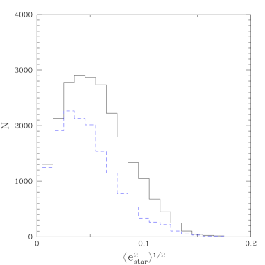
Figure 5: Histogram of the Point Spread Function anisotropy of the stars in the simulated images (solid line) and in the VIRMOS-DESCART survey (dashed line).

and the simulated images reproduce similar observational conditions as real data (PSF anisotropy, limiting magnitude, luminosity functions, galaxy and star number densities, intrinsic ellipticity…). The simulated galaxies are then analyzed exactly in the same way as real data, following the procedure described in (Van Waerbeke et al., 2000, 2001b)

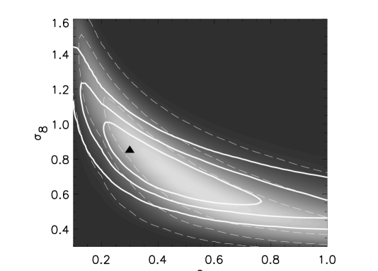
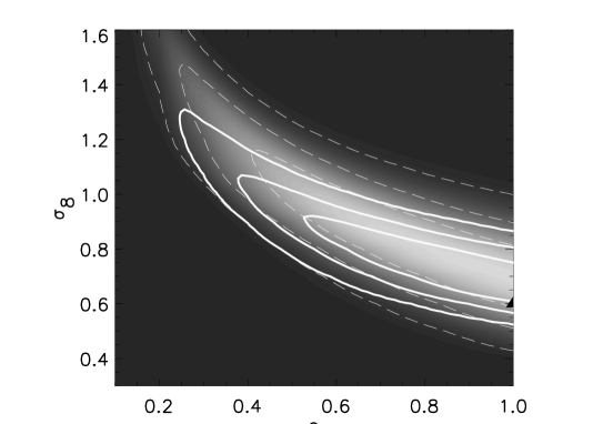
Figure 6: Constraints on $\sigma_{8}$ and $\Omega_{M}$ for the OCDM (left) and $\tau$CDM (right) simulations. The gray levels and the dashed contours show the -simulation- default prior constraints, with confidence levels of $0.68$, $0.95$ and $0.999$. The true model, indicated by a dark triangle, is $\Omega=0.3$, $\sigma_{8}=0.85$ (left) and $\Omega=1$, $\sigma_{8}=0.6$ (right). The thick solid line contours are for a prior $\Gamma\in[0.1,0.3]$ and $\bar{z}_{s}\in[0.9,1.1]$.

We used two ray-tracing simulations from Jain et al. (2000): one is OCDM, as described in Section 3, and the other is a $\tau$CDM with $\Gamma=0.21$ and $\Omega=1$. For each simulation we produced $11$ square degrees of simulated sky images containing roughly $30$ galaxies per arcmin², with a pixel size of $0.2$ arcsec. Figure 5 compare the star anisotropy between the simulated fields (solid line) and the data (dashed line). The likelihood function is computed for 11760 models ($10\times 14\times 14\times 6$). Figure 6 shows the results for the maximum likelihood analysis of these two simulation sets. We clearly converge to the right cosmological model, which validates our likelihood approach for the data (see Section 5.2). However, we should point out here that the likelihood method assumes that our theoretical predictions are accurate compared to the precision of the measurements. Our simulations shows this is unfortunately not necessarily the case with today’s lensing data sets. For instance, it was shown in Van Waerbeke et al. (2001a) (Figure 2), that the non-linear predictions fails badly for the aperture mass with a $\tau$CDM model. This failure should not be a surprise: it was already noticed in the projected power spectrum in Jain et al. (2000) (Figure 8), and even the VIRGO simulations (see Jenkins et al., 1998, Figure 7) already noticed a mismatch between the 3D non-linear predictions and the measured power spectrum. In the case of our $\tau$CDM simulation, the potential problem is an overestimate of the power spectrum normalization $\sigma_{8}$. This is illustrated in Figure 7 where we compare the measured power to the Peacock & Dodds prediction for that model. With a smaller statistical error and/or residual bias and cosmic variance, the true model with $\sigma_{8}=0.6$ will become excluded from our $3-\sigma$ contours in the right panel of figure 6. In fact a maximum likelihood analysis on the noise free catalogue would give $\sigma_{8}=0.8$, that is $20\%$ larger than the true $\sigma_{8}$, which corresponds to the lack of power in the predicted non-linear signal. We will get back to a more detailed discussion in Section 6 about this problem.

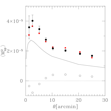
Figure 7: The filled circles with error bars show the aperture mass measured on the $\tau$CDM simulated sky images, while the filled small squares show the signal measured in the input catalogue. The open circles show the measured residual $B$-mode. Measurements and simulation are in perfect agreement, but the non-linear prediction obtained from Peacock & Dodds (1996) for this model (solid line) is significantly off.

5.2 VIRMOS-DESCART data

We first consider flat cosmologies, since this is the class of models currently favored by the cosmic microwave background measurements (de Bernardis et al., 2000), but alternative open universes are also investigated. In either case, the likelihood function is computed for 17640 ($10\times 14\times 14\times 9$) models using Eq.(8), as a function of angular scale, and for a regular spacing in the default prior box.

Figure 8 shows the four parameters constraints for different priors and marginalized parameters for the flat cosmology. The dashed lines shows the $68\%$, $95\%$ and $99.9\%$ contours when the default prior is applied for the two remaining parameters. We cannot extract strong constraints in that case, but the right panel shows an interesting tendency between $\Gamma$ and $z_{s}$: a flat power spectrum (large $\Gamma$) can account for an underestimated source redshift. The thick solid curves shows the same contours with a stronger prior: $\Gamma$ and $z_{s}$ are marginalized over $[0.1,0.4]$ and $[0.39,0.54]$ for the left panel, and $\Omega_{M}$ and $\sigma_{8}$ are marginalized over $[0.1,0.4]$ and $[0.7,1.3]$ for the right panel. We obtain the following constraint from the left panel:

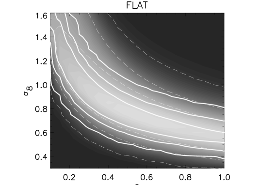
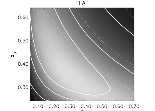
Figure 8: Left: constraints on $\Omega$ and $\sigma_{8}$ for the flat cosmologies. The confidence levels are $[68,95,99.9]$ from the brightest to the darkest area. The galaxy sample has a magnitude cut $m_{I}>21$. The gray area, and the dashed contours correspond to the contours computed with a full marginalization over the default prior $\Gamma\in[0.05,0.7]$ and $z_{s}\in[0.24,0.64]$. The thick solid line contours are obtained from the prior $\Gamma\in[0.1,0.4]$ and $z_{s}\in[0.39,0.54]$ (which is a mean redshift $\bar{z}_{s}\in[0.8,1.1]$). Right: constraints on $\Gamma$ and $\Omega_{M}$ for the flat cosmologies. The contours have the same statistical meaning as for the left panel, but here, the dashed lines correspond to a marginalization over the default prior $\Omega\in[0.1,1]$ and $\sigma_{8}\in[0.3,1.6]$, and the thick lines for $\Omega\in[0.1,0.4]$ and $\sigma_{8}\in[0.7,1.3]$.

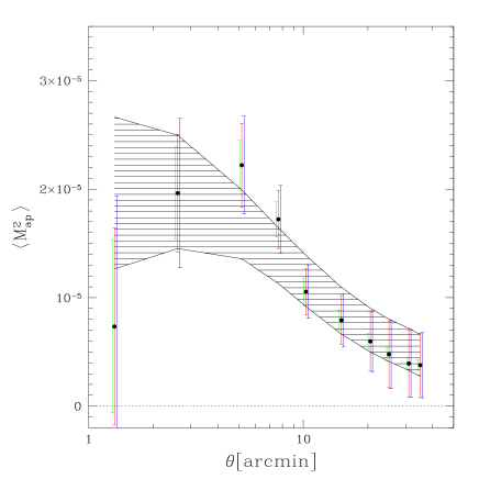
Figure 9: The aperture mass statistic $\langle M_{\rm ap}^{2}\rangle$ measured on the data (see Figure 1) compared to all the models included in the $68\%$ contour (shaded area). For each measurement point, the error bars from left to right are: statistical errors, statistical error and residual bias, statistical errors and bias and cosmic variance.

$$\sigma_{8}=\left(0.57\pm 0.04\right)\Omega_{M}^{\left(0.24\mp 0.18\right)\Omega_{M}-0.49},$$ (15)

for the $68\%$ level and

$$\sigma_{8}=\left(0.58\pm 0.13\right)\Omega_{M}^{\left(0.205\mp 0.025\right)\Omega_{M}-0.48}$$ (16)

for the $95\%$ contour. Constraints on the mass power spectrum can be obtained from the right panel if one assume that photometric redshifts provide the exact redshift distribution (which is given by $z_{s}=0.44$). In that case we have $\Gamma\in[0.12,0.38]$.

Figure 9 shows the aperture mass measurements with all the models inside the $68\%$ contours as the shaded area. The error bars show the contribution the three errors as a function of scale. Each set of errors shows 3 bars, which from left to right are: statistical noise, bias added, cosmic variance added. We see that the statistical noise dominates at small scale, while the systematic residuals dominate at larger scales, the cosmic variance is never an important contribution.

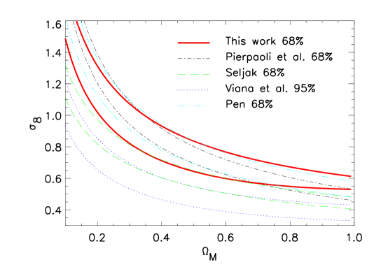
Figure 10: The $\Omega-\sigma_{8}$ constraints for a flat universe from our work, compared to the cluster normalization constraints.

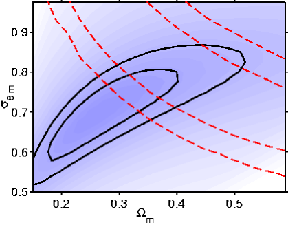
Figure 11: Solid line: the CMB alone constraints as described in Lahav et al. (2001) (figure borrowed from their paper). The CMB priors are given by a concordance model, with the Hubble constant $h=0.7$ with an r.m.s. of $0.07$, the baryon density $\Omega_{b}=0.02$, the primordial spectral index $n=1$, and the reonization depth $\tau=0$. Dashed lines our cosmic shear constraints for the flat cosmologies (see Figure 8). In either case, the contours show the $68\%$ and $95\%$ confidence levels.

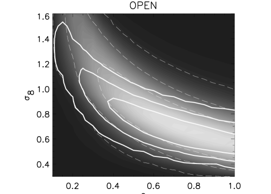
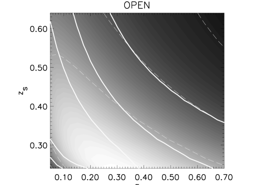
Figure 12: Same as Figure 8 for the open cosmologies.

It is interesting at this stage to compare our results with measurements from other surveys. A comparison with Cosmic Microwave Background (CMB) constraints reveals that weak lensing will be helpfull to break the degeneracy between $\sigma_{8}$ and $\Omega_{M}$. Recently, Lahav et al. (2001) have shown CMB estimation of these two parameters, assuming that the Hubble constant is a Gaussian variable centered at $h=0.7$ with an r.m.s. of $0.07$, and fixing other parameters (primordial spectral index $n=1$, baryon density $\Omega_{b}=0.02$ and reionization depth $\tau=0$). Their results are shown as the solid lines on Figure 11. An overlay of our constraints on the same plot (dashed lines) show that a combination of CMB and lensing would favorise low density models ($\Omega_{M}\sim 0.3-0.4$) and rather low normalisation ($\sigma_{8}\sim 0.7-0.8$). This plot reveals that the lensing constraints are almost orthogonal to the CMB constraints. As explained in Lahav et al. (2001), a weaker prior on $h$ would extend the CMB contours and restore the degeneracy between $\Omega_{M}$ and $\sigma_{8}$, making $\Omega_{M}=1$ a viable solution again. But we see that lensing rules out such a solution because $\Omega_{M}\sim 1$ with $\sigma_{8}>0.8$ is excluded. Given that CMB alone predicts a flat Universe, the inconsistency between CMB and lensing for $\Omega_{M}=1$ should be interpreted as in favor of a non-zero cosmological constant. The fact that CMB and lensing have oposite constraints in the ($\sigma_{8}$,$\Omega_{M}$) parameter space make them indeed very complementary. A complete analysis which take into account the marginalization over the other parameters (baryon density, $\tau$, etc…) is under way. However, we should note the agreement between our results and the combined CMB+2dF contraints (Lahav et al., 2001, Figure 5).

We should also compare our results more closely to the cluster normalization constraints, since those two methods are expected to probe a similar combination of $\sigma_{8}$ and $\Omega_{M}$. Figure 10 shows our results and those obtained from cluster measurements. As it was claimed before (Maoli et al., 2001; Van Waerbeke et al., 2001b; Rhodes et al., 2001), a joint estimate of $\Omega_{M}$ and $\sigma_{8}$ from weak lensing is consistent with the former cluster abundance estimates (Pen, 1998; Pierpaoli et al., 2001). Recently, these estimates were revisited but the new results are puzzling (see Figure 10): whereas Seljak (2001) is marginaly consistent with our constraints, on the other hand, Viana et al. (2001) is significantly lower. Pen (1998) performed direct hydrodynamic simulations to predict the cluster X-ray temperature function for various cosmological models. This bypasses the difficult mass ladder, of converting N-body or Press-Schechter mass functions into a temperature function, and/or accounting for scatters in the relation, and the results are in good agreement with the cosmic shear constraints. However, some effects that may still not be accounted for in simulations include non-gravitational feedback from galaxies, magnetic fields, thermal conduction, which may all limit the intrinsic accuracy of cluster normalizations. We will not enter into the debate between the cluster estimates here, but if the low normalization is confirmed, this discrepancy might be an important finding: it might be an indication of the inaccuracy of the non-linear predictions, as shown in Section 5.1.

The maximum likelihood analysis was also carried out for open cosmologies. The probability contours shown in Figure 12 summarize the results which are indeed similar to the flat case. However, low density ($\Omega_{M}<0.2$), open universes, seem more difficult to reconcile with the data than flat models. This contradiction between observations and low density open universe results mostly from the small scale measurement of $\langle M_{ap}^{2}\rangle$ (Figure 9). Indeed, low density open universes predict too much power at small scale as compared to what can be allowed from the amplitude of $\langle M_{ap}^{2}\rangle$ on scale of about one arc-minute. This clear difference between open and flat $\Lambda$CDM universes was already pointed out by Schneider et al. (1998) (Fig. 3) but this is the first time that it manifests on real data.

Finally, although uncertainties are still large enough to leave room for a large sample of models, it is interesting to show how cosmic shear data can be used jointly with several independent surveys (not only CMB). Because weak lensing analyses probe dark matter in a direct way, cosmic shear are the best suited surveys to constrain $\sigma_{8}$. It is then relevant to only focus on this parameter, using values of other cosmological parameters as they are derived from external data sets. Assuming the mean redshift of sources is $z_{s}=0.9$ and $h=0.7\pm 0.1$ (Freedman et al., 2001, from the HST Key Project), a flat universe (from CMB data) with a baryon fraction inferred from BBN and $\Gamma=0.2\pm 0.05$ (Szalay et al., 2002, from the SDSS redshift survey), we then have $\Omega_{M}\approx 0.3\pm 0.1$. In that case, the VIRMOS-DESCART cosmic shear survey provide $\sigma_{8}=0.98\pm 0.06$, in good agreement with other independent methods. As compared to the join CMB-cosmic shear alone discussed previously, the normalisation is higher. This is mainly due to the low $\Omega_{M}$ (i.e. high $\sigma_{8}$) combined with a strong prior on $\Gamma$ (inferred from the galaxy redshift survey) and on the source redshift.

6 Conclusion

We explored a 4-dimensional parameter space using the most recent cosmic shear data. We included all possible sources of error: statistical noise, cosmic variance and residual systematics. We obtained constraints on $\Omega_{M}$, the power spectrum slope $\Gamma$, its normalization $\sigma_{8}$ and the redshift of the sources $z_{s}$. We marginalized over $\Gamma$ and $z_{s}$. Both the marginalization, and the inclusion of all the sources of error, make our results for $(\Omega_{M},\sigma_{8})$ robust. We pointed out the complementarity between cosmic shear and CMB measurements for breaking the degeneracy among $\Omega_{M}$ and $\sigma_{8}$, and the good agreement with CMB and CMB+2dF constraints. However, our results are only in marginal agreement with the latest cluster abundance constraints, which give a lower normalization $\sigma_{8}\sim 0.7$ for $\Omega_{M}\sim 0.3$. If this discrepancy is confirmed in either measurements, this could be interpreted as an indication that the lensing non-linear prediction is not accurate enough given the already small size of cosmic shear errors. This interpretation is supported by ray-tracing simulations in a $\tau$CDM model, and more generaly by a comparison of the VIRGO simulations with the Peacock & Dodds non-linear prescription. It was claimed a $15\%$ accuracy in their original paper (Peacock & Dodds, 1996), although it might be a bit more for some cosmological models (Jenkins et al., 1998). This is clearly the maximum uncertainty we can tolerate with today’s lensing measurements, and it will be insufficient for forthcoming surveys. This potential problem suggests three paths for improvements:

1. Ray-tracing simulations should be used more intensively to test non-linear schemes. So far, simple ray-tracing have been performed, by putting all the sources at a single redshift ($z_{s}=1$), although in principle we should expect a redshift dependence of the non-linear predictions failure (because different physical scales are probes for a varying redshift, for a fixed angular scale).

2. Progress on the theory side should be done. There might be some hope by reviving the halo models which give predictions close, but not identical, to Peacock & Dodds (like the peakpatch approach, Bond, priv. comm.).

3. Ultimately, cosmic shear observations will lead to a measurement of the 3D mass power spectrum in non-parametric way, and therefore solve all the problems associated with non-linear modeling. This is possible only if the cosmological parameters are determined by other means. For instance, the linear mass power spectrum and cosmological parameters measurement at large scales using combined (or not) lensing data with cosmic microwave background, X-rays, could be obtained, and used to deconvolve the non-linear power spectrum. This means that we will be able to deconvolve the projected mass power spectrum measured from cosmic shear observations and recover the true 3D power spectrum. This is a work in progress, in which we are trying to recover the galaxy-galaxy and galaxy-mass correlations as well, using tomography techniques (Hu, 1999).