Cosmic microwave background and large scale structure limits on the interaction between dark matter and baryons

Abstract

We study the effect on the cosmic microwave background (CMB) anisotropy and large scale structure (LSS) power spectrum of a scattering interaction between cold dark matter and baryons. This scattering alters the CMB anisotropy and LSS spectrum through momentum transfer between the cold dark matter particles and the baryons. We find that current CMB observations can put an upper limit on the scattering cross section which is comparable with or slightly stronger than previous disk heating constraints at masses greater than 1 GeV, and much stronger at smaller masses. When large-scale structure constraints are added to the CMB limits, our constraint is more stringent than this previous limit at all masses. In particular, a dark matter-baryon scattering cross section comparable to the “Spergel-Steinhardt” cross section is ruled out for dark matter mass greater than 1 GeV.

I Introduction

It is now generally accepted that the energy density of the universe includes a substantial fraction of cold dark matter (CDM), constituting roughly $0.3-0.4$ of the closure density. It is normally assumed that the CDM particle does not interact with ordinary baryonic matter or with photons; hence the “dark” in cold dark matter. However, a small scattering cross section cannot be entirely ruled out, only constrained by observations.

Several different models are possible for interactions between ordinary matter and CDM. One possibility is strongly interacting dark matter (also known as strongly interacting massive particles, or SIMPs), in which the CDM particle couples to baryons, but not to photons or electrons. Recently, to solve the small scale problem in CDM models, strongly self-interacting particles were suggested Spergel ; Wandelt , with

$$8\times 10^{-25}<\frac{\sigma/{\rm cm}^{2}}{m/{\rm GeV}}<10^{-23}.$$ (1)

The range quoted here (from Ref. Wandelt ) is narrower than originally proposed in Spergel because of additional constraints. While the original Spergel-Steinhardt cross section applies only to dark matter self-interaction, if such an interaction is mediated by the strong force, then the dark matter might also interact strongly with baryonsWandelt . Examples of such dark matter includes, e.g., quark-gluino bound states Farrar , strangelets Jaffe , gauge singlet mesons Bento , and Q-balls Kusenko . Limits on such interactions were investigated by Starkman et al. Starkman , and recently reexamined in references Wandelt ; QW ; Moh ; Cyburt . A second possibility is to couple the dark matter particle electromagnetically, e.g., by giving it a tiny electromagnetic charge (see, e.g., reference millicharge and references therein); such a CDM particle will scatter primarily off of photons and free electrons.

Any interactions of this sort will affect the spectrum of the cosmic microwave background (CMB) fluctuations, since they act to transfer momentum from the dark matter to the baryon-photon fluid, although for WIMPs this effect is negligible Chen ; Hofmann . Current CMB observations can place constraints on such models. The case of direct interactions between the CDM particle and photons has already been examined Boehm , so we do not consider it here. While the model discussed in reference Boehm is not identical to the case of electromagnetically charged dark matter, since it includes photon-CDM interactions but not electron-CDM interactions, we expect it to be qualitatively similar to the charged dark matter model. Therefore, we consider only the case of strongly-interacting dark matter, in which the dark matter particle couples to baryons (only).

In the next section, we give the perturbation equations for CDM which couples to baryons, and we show the matter transfer function and CMB power spectra for some representative cases. In Sec. 3, we compare our calculations with the CMB observations to derive constraints on the cross section for dark matter-baryon scattering, and we compare to previously-derived limits. Our conclusions are summarized in Sect. 4.

II Fluctuation growth with strongly-interacting dark matter

II.1 The Basic Modified Equations

We begin by assuming a scattering cross section $\sigma$ between the CDM particle of mass $m_{c}$ and protons with mass $m_{b}$, and we derive the changes to the perturbation equations produced by this scattering interaction. Our starting point is the set of perturbation equations in reference MB95 , which form the basis for CMBFAST CMBFAST . We will not reproduce here all of the perturbation equations, but simply give those equations which are modified.

Following reference MB95 , we work in the synchronous gauge. However, because the CDM is interacting it does not provide a natural way of defining the synchronous coordinates, as opposed to standard CDM MB95 . Let $\delta_{c}$ and $\delta_{b}$ be the density fluctuation ($\equiv\delta\rho/\rho$) for the cold dark matter and the baryons, respectively, and let $\theta_{c}$ and $\theta_{b}$ be the corresponding velocity divergences. Then for the cold dark matter, we have

$$\dot{\delta}_{c} = -\theta_{c}-\frac{1}{2}\dot{h},$$ (2)

$$\dot{\theta}_{c} = -\frac{\dot{a}}{a}\theta_{c}+c_{c}^{2}k^{2}\delta_{b}+R_{c}$$ (3)

For baryons the corresponding terms are

$$\dot{\delta}_{b} = -\theta_{b}-\frac{1}{2}\dot{h},$$ (4)

$$\dot{\theta}_{b} = -\frac{\dot{a}}{a}\theta_{b}+c_{b}^{2}k^{2}\delta_{b}+R_{\gamma}+R_{b}.$$ (5)

with

$$R_{b} \equiv K_{c}(\theta_{b}-\theta_{c})=\frac{m_{c}n_{c}\sigma v_{\rm rel}a}{m_{b}+m_{c}}(\theta_{b}-\theta_{c}),$$ (6)

$$R_{c} \equiv K_{b}(\theta_{c}-\theta_{b})=\frac{m_{b}n_{b}\sigma v_{\rm rel}a}{m_{b}+m_{c}}(\theta_{c}-\theta_{b}),$$ (7)

$$R_{\gamma} \equiv K_{\gamma}(\theta_{\gamma}-\theta_{b})=\frac{4\rho_{\gamma}}{3\rho_{b}}an_{e}\sigma_{T}(\theta_{\gamma}-\theta_{b})$$ (8)

In these equations $c_{c}$ and $c_{b}$ are the adiabiatic sound speed of the CDM and baryons, respectively, $v_{\rm rel}$ is the average relative velocity between the CDM and the baryons, and $R_{c},R_{b},R_{\gamma}$ are the momentum transfer terms. The sound speeds are given by

$$c_{b}^{2} = (k_{B}T_{b}/\mu)\left(1-\frac{1}{3}\frac{d\ln T_{b}}{d\ln a}\right),$$ (9)

$$c_{c}^{2} = (k_{B}T_{c}/m_{c})\left(1-\frac{1}{3}\frac{d\ln T_{c}}{d\ln a}\right),$$ (10)

the average relative velocity by

$$v_{\rm rel}=\sqrt{\frac{3(m_{c}T_{b}+m_{b}T_{c})}{m_{b}m_{c}}},$$ (11)

In calculating average velocities we have assumed thermal Maxwell-Boltzmann distributions for both CDM and baryons. The temperature evolution of the dark matter and baryons is given by

$$\dot{T}_{b}+2\frac{\dot{a}}{a}T_{b} = -K_{\gamma}(T_{b}-T_{\gamma})-K_{c}(T_{b}-T_{c}),$$ (12)

$$\dot{T}_{c}+2\frac{\dot{a}}{a}T_{c} = -K_{b}(T_{c}-T_{b}).$$ (13)

It is possible to obtain analytical solutions for the temperature evolution equations, but they are complicated and cumbersome to use. Instead, we use a semi-implicit scheme to integrate these differential equations. We tested this method in a few cases, and found that it produces solutions which agree with the analytical solutions within 0.2%, and the effect on the CMB spectrum is negligible.

II.2 The Effect of Primordial Helium

This set of equations ignores the fact that the baryonic fluid consists of two species: hydrogen and helium-4, in a roughly 3 to 1 ratio by mass. To account for the presence of helium as well as hydrogen, we make the following replacements:

$$\frac{m_{b}n_{b}\sigma v_{\rm rel}}{m_{b}+m_{c}} \rightarrow \frac{m_{\rm H}n_{\rm H}\sigma_{\rm H}v_{\rm H}}{m_{\rm H}+m_{c}}+\frac{m_{\rm He}n_{\rm He}\sigma_{\rm He}v_{\rm He}}{m_{\rm He}+m_{c}},$$ (14)

$$\frac{m_{c}n_{c}\sigma v_{\rm rel}}{m_{b}+m_{c}} \rightarrow \frac{m_{c}n_{c}\sigma_{\rm H}v_{\rm H}}{m_{\rm H}+m_{c}}(1-Y)+\frac{m_{c}n_{c}\sigma_{\rm He}v_{\rm He}}{m_{\rm He}+m_{c}}Y,$$ (15)

where $Y$ is the primordial mass fraction of helium-4 (we take $Y=0.24$ throughout), and we define separate velocities for the hydrogen and helium relative to the dark matter:

$$v_{\rm H} = \sqrt{\frac{3(m_{c}T_{b}+m_{\rm H}T_{c})}{m_{\rm H}m_{c}}}$$ (16)

$$v_{\rm He} = \sqrt{\frac{3(m_{c}T_{b}+m_{\rm He}T_{c})}{m_{\rm He}m_{c}}}.$$ (17)

In our calculations, $\sigma$, the scattering cross section between the CDM particle and the proton, is a free parameter which we will constrain from the observations. However, we need to make some sort of assumption regarding $\sigma_{He}$, the scattering cross section between CDM and helium nuclei. For coherent scattering, we expect $\sigma_{He}=16\sigma$, while a spin-dependent cross section would yield $\sigma_{He}=0$. For now, we will examine the intermediate case of incoherent scattering, for which $\sigma_{He}=4\sigma$. Later, in Sec. 3, we will extend our calculation to consider both coherent scattering and spin-dependent scattering.

Taking $m_{\rm He}\simeq 4m_{\rm H}$, and $n_{b}=\rho_{b}/m_{\rm H}$, the above substitution can be achieved by simply replacing everywhere

$$\frac{m_{b}\sigma v_{\rm rel}}{m_{b}+m_{c}} \longrightarrow \frac{m_{\rm H}\sigma}{m_{\rm H}+m_{c}}\left[(1-Y)v_{\rm H}+Y\left(\frac{\sigma_{\rm He}}{\sigma_{\rm H}}\right)\frac{m_{\rm H}+m_{c}}{4m_{\rm H}+m_{c}}v_{\rm He}\right]$$ (18)

$$\frac{m_{c}\sigma v_{\rm rel}}{m_{b}+m_{c}} \longrightarrow \frac{m_{c}\sigma}{m_{\rm H}+m_{c}}\left[(1-Y)v_{\rm H}+Y\left(\frac{\sigma_{\rm He}}{\sigma_{\rm H}}\right)\frac{m_{\rm H}+m_{c}}{4m_{\rm H}+m_{c}}v_{\rm He}\right].$$ (19)

II.3 Tight-Coupling Approximation

Following reference MB95 , we use a separate set of equations in the limit of tight coupling between baryons and photons. In the tight-coupling regime, the temperature evolution is given by

$$\dot{T}_{b} = -2\frac{\dot{a}}{a}T_{b}+\frac{8}{3}\frac{\mu}{m_{e}}\frac{\rho_{\gamma}}{\rho_{b}}an_{e}\sigma_{T}(T_{\gamma}-T_{b})+K_{c}(T_{c}-T_{b})$$ (20)

$$\dot{T}_{c} = -2\frac{\dot{a}}{a}T_{c}+K_{b}(T_{b}-T_{c})$$ (21)

where $\mu$ is the mean molecular weight. During tight coupling, $T_{c}\sim T_{b}\sim T_{\gamma}$, $\dot{T_{b}}\sim-\frac{\dot{a}}{a}T_{b}$, and $\dot{v}_{\rm rel}=-\frac{1}{2}\frac{\dot{a}}{a}v_{\rm rel}$. Setting $R=4\rho_{\gamma}/3\rho_{b}$, and $\tau_{\gamma}=(an_{e}\sigma_{T})^{-1}$, we have

$$\dot{R}_{b}+\frac{\dot{a}}{a}R_{b}=\frac{m_{c}n_{c}\sigma av_{\rm rel}}{m_{b}+m_{c}}\left[(\dot{\theta}_{c}-\dot{\theta}_{b})-\frac{3}{2}\frac{\dot{a}}{a}(\theta_{c}-\theta_{b})\right]$$ (22)

$$(1+R)\dot{\theta_{b}}+\frac{\dot{a}}{a}\theta_{b}-c_{b}^{2}k^{2}\delta_{b}-k^{2}R\left(\frac{1}{4}\delta_{\gamma}-\sigma_{\gamma}\right)+R(\dot{\theta}_{\gamma}-\dot{\theta}_{b})-R_{b}=0,$$ (23)

$$\theta_{b}-\theta_{\gamma}=\frac{\tau_{\gamma}}{1+R}\left[-\frac{\dot{a}}{a}\theta_{b}+k^{2}(c_{b}^{2}\delta_{b}-\frac{1}{4}\delta_{\gamma}+\sigma_{\gamma})+\dot{\theta}_{\gamma}-\dot{\theta}_{b}+R_{b}\right],$$ (24)

$$\dot{\theta}_{b}-\dot{\theta}_{\gamma}=\frac{\tau_{\gamma}}{1+R}\left[-\frac{\ddot{a}}{a}\theta_{b}-\frac{\dot{a}}{a}k^{2}\frac{\delta_{\gamma}}{2}+k^{2}\left(c_{b}^{2}\dot{\delta}_{b}-\frac{1}{4}\dot{\delta}_{\gamma}\right)+\frac{\dot{a}}{a}R_{b}+\dot{R}_{b}\right]+\frac{2R}{1+R}\frac{\dot{a}}{a}\left(\theta_{b}-\theta_{\gamma}\right).$$ (25)

II.4 Applicable range of our calculation

In the calculation described above, we have assumed that the dark matter is made of a single type of particle, with density parameter $\Omega_{m}$. We have also assumed that it is a “cold dark matter” particle, i.e. during the whole range of our calculation it is non-relativistic, which translates to $m>1$ MeV. We have also assumed that during each scattering only one baryon interacts with the dark matter particle. If the interaction length of the particle is $a$ ($\sigma\equiv 4\pi a^{2}$), then we require that this interaction length be less than the inter-particle spacing:

$$a<n_{b}^{-1/3},$$ (26)

where $n_{b}\sim 10^{-5}(1+z)^{3}h_{0}^{2}\Omega_{b}{\rm cm}^{-3}$. Processes which affect CMB anisotropy happen at redshift less than $10^{5}$, so we can put a limit on the applicable cross section, neglecting factors of order unity:

$$\sigma_{\rm max}\sim 10^{-6}{\rm cm}^{2}.$$ (27)

Our calculation must be modified for $\sigma>\sigma_{\rm max}$ to take into account multi-particle scattering.

II.5 The matter and CMB power spectra

We have modified the CMBFAST code CMBFAST to include the effects discussed in the previous sections. For initial conditions, we assume that the dark matter and baryons started tightly coupled with the same temperature. Tensor modes have been ignored, and we consider only flat geometries ($\Omega=1$).

In Fig. 1 we show the CMB fluctuation spectra and the corresponding square of the matter transfer function for some representative cases. The coupling of the dark matter to the baryons damps the matter power spectrum on small scales, as can be seen in Fig.  1(b).

One might imagine that the effect on the CMB of coupling the baryons to the dark matter would be equivalent to a standard model with a larger value of $\Omega_{b}$. This is not the case, as can be seen in Fig. 1(a). Although both models produce an increase in the amplitude of the first acoustic peak, the large $\Omega_{b}$ model produces an increase in the amplitude of the third peak, while the strongly-interacting dark matter model yields a decrease in the third peak amplitude (and in all of the other peaks as well).

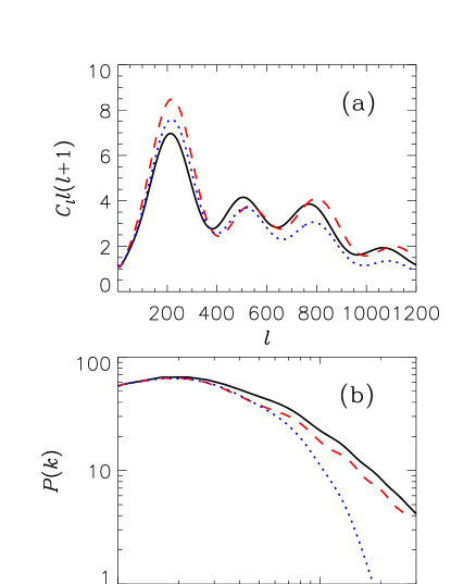
Figure 1: (a) CMB power spectra for a few sample cases. The solid (black) curve is a fiducial $\Lambda$CDM model with parameters $\Omega=1$, $\Omega_{b}h^{2}=0.018$, $\Omega_{m}h^{2}=0.18$, $H_{0}=75\,\,{\rm km}\,{\rm s}^{-1}\,{\rm Mpc}^{-1}$, $n=1$, and without dark matter-baryon interaction. The dotted (blue) curve is for a dark matter mass of 1 GeV, with a dark matter-baryon cross section $\sigma=3\times 10^{-24}\,\,{\rm cm}^{2}$. The dashed (red) curve is for a model without dark matter-baryon interaction, but with increased baryon density, $\Omega_{b}=0.05$. All spectra are calculated without COBE-normalization (arbitrary units) and taking $\sigma_{He}=4\sigma$. (b) Matter power spectra for the same models as in (a). Normalization is arbitrary.

One can understand the difference between the CMB spectra in the following way: The baryon-photon oscillations are damped oscillations, with a damping rate (viscosity) inversely proportional to the baryon-photon interaction rate. Interacting CDM with intermediate cross section amounts to adding “baryons” but simultaneously also increasing the viscosity of the plasma. Therefore the acoustic oscillations damp quickly and all peaks but the first are suppressed. Scales around the first acoustic peak have only undergone part of an oscillation and therefore have not been damped significantly. On such large scales the increase in oscillation amplitude due to added “baryons” is more important and the overall power spectrum increases.

On the other hand, increasing the baryon density has the well-known effect of increasing the height of the compression peaks (1st, 3rd,…) and decreasing the height of the decompression peaks (2nd, 4th,…). Of course, for very large cross sections, the effective viscosity of the CDM-baryon-photon plasma approaches that of a pure baryon-photon plasma and the CDM acts exactly like baryons. An effect similar to the increased viscosity due to CDM-baryon interactions can be seen in models with increased width of the last scattering surface due to non-standard recombination, where the effective viscosity of the baryon-photon plasma also increases around the time of recombination HS01 .

The effect on the matter power spectrum seen in Fig. 1(b) can be understood in the same way. The increased viscosity in the interacting model leads to a much stronger damping on small scales than in the model with increased baryon density.

III Comparison with observations

In order to constrain models with CDM-baryon interactions we compare the CMB and matter power spectra of such models with recent observational data.

CMB data set — Several data sets of high precision are now publicly available. In addition to the COBE Bennett:1996ce data for small $l$ there are data from BOOMERANG boom , MAXIMA max , DASI dasi and several other experiments WTZ ; qmask . Wang, Tegmark and Zaldarriaga WTZ have compiled a combined data set from all these available data, including calibration errors. In the present work we use this compiled data set, which is both easy to use and includes all relevant present information.

LSS data set — At present, by far the largest survey available is the 2dF 2dF of which about 147,000 galaxies have so far been analysed. Tegmark, Hamilton and Xu THX have calculated a power spectrum, $P(k)$, from this data, which we use in the present work. The 2dF data extends to very small scales where there are large effects of non-linearity. Since we only calculate linear power spectra, we use (in accordance with standard procedure) only data on scales larger than $k=0.2h\,\,{\rm Mpc}^{-1}$, where effects of non-linearity should be minimal.

The CMB fluctuations are usually described in terms of the power spectrum, which is again expressed in terms of $C_{l}$ coefficients as $l(l+1)C_{l}$, where

$$C_{l}\equiv\langle|a_{lm}|^{2}\rangle.$$ (28)

The $a_{lm}$ coefficients are given in terms of the actual temperature fluctuations as

$$T(\theta,\phi)=\sum_{lm}a_{lm}Y_{lm}(\theta,\phi).$$ (29)

Given a set of experimental measurements, the likelihood function is

$${\cal L}(\Theta)\propto\exp\left(-\frac{1}{2}x^{\dagger}[C(\Theta)^{-1}]x\right),$$ (30)

where $\Theta=(\Omega,\Omega_{b},H_{0},n,\tau,\ldots)$ is a vector describing the given point in parameter space, $x$ is a vector containing all the data points, and $C(\Theta)$ is the data covariance matrix. This applies when the errors are Gaussian. If we also assume that the errors are uncorrelated, it can be reduced to the simple expression, ${\cal L}\propto e^{-\chi^{2}/2}$, where

$$\chi^{2}=\sum_{i=1}^{N_{\rm max}}\frac{(C_{l,{\rm obs}}-C_{l,{\rm theory}})_{i}^{2}}{\sigma(C_{l})_{i}^{2}},$$ (31)

is a $\chi^{2}$-statistic and $N_{\rm max}$ is the number of power spectrum data points oh . In the present letter we use equation (31) for calculating $\chi^{2}$. In the case where we also use LSS data $\chi^{2}$ is instead given by

$$\chi^{2}=\sum_{i=1}^{N_{\rm max,CMB}}\frac{(C_{l,{\rm obs}}-C_{l,{\rm theory}})_{i}^{2}}{\sigma(C_{l})_{i}^{2}}~{}~{}~{}+\sum_{j=1}^{N_{\rm max,LSS}}\frac{(P(k)_{{\rm obs}}-P(k)_{{\rm theory}})_{j}^{2}}{\sigma(P(k))_{j}^{2}}.$$ (32)

The procedure is then to calculate the likelihood function over the space of cosmological parameters. The 2D likelihood function for $(m_{c},\sigma)$ is obtained by keeping $(m_{c},\sigma)$ fixed and marginalising over all other parameters.

As free parameters in the likelihood analysis we use $\Omega_{m}$, the matter density, $\Omega_{b}$, the baryon density, $H_{0}$, the Hubble parameter, $n$, the scalar spectral index, $\tau$, the optical depth to reionization, and $Q$, the overall normalization of the data. When large scale structure constraints are included we also use $b$, the normalization of the matter power spectrum, as a free parameter. This means that we treat $Q$ and $b$ as free and uncorrelated parameters. This is very conservative and eliminates any possible systematics involved in determining the bias parameter. We constrain the analysis to flat ($\Omega_{m}+\Omega_{\Lambda}=1$) models, and we assume that the tensor mode contribution is negligible ($T/S=0$). These assumptions are compatible with analyses of the present data WTZ , and relaxing them does not have a big effect on the final results. For maximizing the likelihood function we use a simulated annealing method, as described in reference Hannestad:2000wx .

Table I shows the different priors used. In the “CMB” prior the only important constraint is that $0.4\leq h\leq 0.9$ ($h\equiv H_{0}/(100\,\,{\rm km}\,{\rm s}^{-1}\,{\rm Mpc}^{-1})$). For the CMB+$H_{0}$+BBN prior we use the constraint $H_{0}=72\pm 8\,\,{\rm km}\,{\rm s}^{-1}\,{\rm Mpc}^{-1}$ from the HST Hubble key project freedman (the constraint is added assuming a Gaussian distribution) and the constraint $\Omega_{b}h^{2}=0.020\pm 0.002$ from BBN Burles:2000zk . Finally, in the $H_{0}$+BBN+LSS case, we add data from the 2dF survey THX .

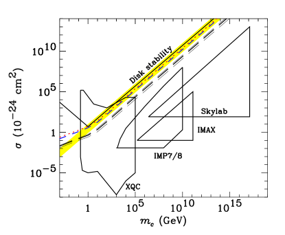
Figure 2: Excluded regions in the $(m_{c},\sigma)$ plane for strongly-interacting dark matter, where $m_{c}$ is the mass of the dark matter particle, and $\sigma$ is the cross section for scattering between dark matter and protons. Dashed and dotted lines are the CMB limits derived in this paper with various priors: dotted (red) is CMB only, short-dash (blue) is CMB+BBN+$H_{0}$, thick long-dash (black) is CMB+BBN+$H_{0}$+LSS. All of these limits assume a scattering cross-section between helium and dark matter of $\sigma_{He}=4\sigma$. Thin dashed lines give the limits for CMB+BBN+$H_{0}$+LSS for spin-dependent scattering between helium and dark matter ($\sigma_{He}=0$, upper curve) and coherent scattering ($\sigma_{He}=16\sigma$, lower curve). In all of these cases, the region above the curve is excluded at the 95% confidence level. Solid lines give excluded regions from other papers. The region above the top solid line is excluded by the disk heating constraint from Starkman et al. Closed solid contours give excluded regions from the indicated space and balloon-based experiments discussed by Wandelt et al. The regions enclosed by these curves are excluded. The shaded (yellow) strip is the region suggested in Wandelt et al. for which self-interacting dark matter would have a comparable cross section for scattering off of both baryons and itself.

Following Ref. Wandelt , we plot the constraints from various experiments in the $(m_{c},\sigma)$ plane in Fig. 2; limits obtained with different priors are plotted with different line styles. The shaded region is the “Spergel-Steinhardt” region as given in equation (1); note that it is actually narrower than plotted in Fig. 3 of Ref. Wandelt . This figure clearly shows that constraints from the CMB data alone for large CDM mass ($m_{c}>m_{b}\sim 1$ GeV) are comparable to limits from galactic disk heating arguments Starkman . On the other hand, for small CDM mass ($m_{c}<m_{b}\sim 1$ GeV), the limit from the CMB alone is much stronger. This difference arises because the limits from disk heating are related to energy transfer, which decreases as $(m_{c}/m_{b})^{2}$ for $m_{c}\ll m_{b}$, while the limits from the CMB and large scale structure are based on momentum transfer, which decreases only as $m_{c}/m_{b}$ for $m_{c}\ll m_{b}$. At the same time, the relative velocity also increases for low CDM mass (as $m_{c}^{-1/2}$). This is the reason that, for $m_{c}\ll m_{b}$, our bound goes as $m_{c}^{1/2}$, but for the disk heating argument it goes as $m_{c}^{-1}$. Our bound is therefore much stronger at low mass, even if only CMB data is used.

The addition of priors on $\Omega_{b}$ and $H_{0}$ does not increase the exclusion region by much, because there is very little degeneracy between $(m_{c},\sigma)$ and these two parameters. Only when LSS data is added do we find a significant improvement. The reason is that CDM-baryon interactions lead to a significant suppression of small scale power, as discussed in the previous section. Even for relatively small cross sections this effect leads to a disagreement with the 2dF data. With the inclusion of LSS data, our bound becomes much stronger than the disk heating argument of Starkman et al. Starkman , even at large masses. A good analytical fit to our 95% C.L. limit is

$$\frac{\sigma}{10^{-24}{\rm cm^{2}}}<\frac{0.63x^{1/2}+0.22x^{3/2}}{1+x^{1/2}}$$ (33)

where $x=m_{c}$/GeV. Equation (33) is accurate to within 10%. For this case, we also consider the effect of coherent ($\sigma_{He}=16\sigma$) and spin-dependent ($\sigma_{He}=0$) scattering between the dark matter and helium. The limits for these two cases are shown in Fig. 2 as thinner dashed curves above (for $\sigma_{He}=0$) and below (for $\sigma_{He}=16\sigma$) the limit for $\sigma_{He}=4\sigma$. Altering $\sigma_{He}$ in this way changes the upper bounds by a factor of roughly $2-3$, which is barely noticeable on the scale of this graph.

IV Conclusions

CMB observations constrain any scattering interaction between dark matter and baryons. Our results indicate that the limit from current CMB observations is comparable to previous limits from disk heating Starkman for masses greater than 1 GeV, and the CMB limit is much stronger at smaller masses. If we also include large-scale structure data, then our limit is more stringent that the disk-heating limit at all masses. An analytical fit of our combined CMB+LSS limit is given in Eq. (33).

Our CBM+LSS limits exclude the region discussed in Ref. Wandelt , in which self-interacting dark matter interacts with baryons with roughly the same cross section with which it interacts with itself (Fig. 2). This, by itself, does not exclude the self-interacting dark matter scenario, since the dark matter is not required to interact with baryons at all, but it does exclude models with the indicated dark matter-baryon scattering cross section.

While space and balloon-based experiments can provide tighter constraints for specific regions in the parameter space of CDM mass and cross section, (Fig. 2 and reference Wandelt ), the combination of CMB and large-scale structure appears to provide the best general upper limit on the CDM-baryon scattering cross section for arbitrary CDM masses (and it is much stronger than all other limits at low masses). Our constraints are somewhat stronger for coherent scattering from helium nuclei and weaker for a spin-dependent interaction. Perhaps more importantly, these limits will only get better with new CMB data.

Table 1: The different priors used in the analysis. Notice that in the first two cases, the bias parameter $b$ is not used because LSS data is not included in the fit.

prior type	$\Omega_{m}$	$\Omega_{b}h^{2}$	$h$	$n$	$\tau$	$Q$	$b$
CMB	$\Omega_{b}$-1	0.008 - 0.040	0.4-1.0	0.66-1.34	0-1	free	not used
CMB + BBN + $H_{0}$	$\Omega_{b}$-1	$0.020\pm 0.002$	$0.72\pm 0.08$	0.66-1.34	0-1	free	not used
CMB + BBN + $H_{0}$ + LSS	$\Omega_{b}$-1	$0.020\pm 0.002$	$0.72\pm 0.08$	0.66-1.34	0-1	free	free