The abundance and clustering of dark haloes in the standard $\Lambda$CDM cosmogony

Abstract

Much evidence suggests that we live in a flat Cold Dark Matter universe with a cosmological constant. Accurate analytic formulae are now available for many properties of the dark halo population in such a Universe. Assuming current “concordance” values for the cosmological parameters, we plot halo abundance against redshift as a function of halo mass, of halo temperature, of the fraction of cosmic matter in haloes, of halo clustering strength, and of the clustering strength of the $z=0$ descendants of high redshift haloes. These plots are useful for understanding how nonlinear structure grows in the model. They demonstrate a number of properties which may seem surprising, for example: $10^{9}\,\rm M_{\odot}$ haloes are as abundant at $z=20$ as $L_{*}$ galaxies are today; $10^{6}$K haloes are equally abundant at $z=8$ and at $z=0$; 10% of all matter is currently in haloes hotter than 1 keV, while more than half is in haloes too cool to trap photo-ionized gas; 1% of all matter at $z=15$ is in haloes hot enough to ionise hydrogen; haloes of given mass or temperature are more clustered at higher redshift; haloes with the abundance of present-day $L_{*}$ galaxies are equally clustered at all $z<20$; the metals produced by star-formation at $z>10$ are more clustered at $z=0$ than are $L_{*}$ galaxies.

1 INTRODUCTION

Over the last 20 years the Cold Dark Matter (CDM) cosmogony set out by Peebles (1982), Blumenthal et al. (1984) and Davis et al. (1985) has become the standard model for structure formation in the Universe. It assumes the cosmic mass budget to be dominated by an as yet unidentified, weakly interacting massive particle, whose gravitational effects build structure from an initially Gaussian distribution of adiabatic fluctuations. All structure originated as quantum zero-point fluctuations during an early period of inflationary expansion (see Guth 1997 for a review). CDM models are specified by a small set of parameters. These are the fractions of the current critical density in CDM ($\Omega_{\rm CDM,0}$), in baryons ($\Omega_{\rm B,0}$), and in the cosmological constant ($\Omega_{\Lambda,0}$), the current expansion rate, specified by Hubble’s constant $H_{0}=100h\,{\rm{km\,s^{-1}}}\,{\rm{Mpc}}^{-1}$, and the power spectrum of the initial density fluctuations. Over the wavenumber range of interest, the latter can be approximated by a power-law $P_{i}(k)=Ak^{n}$ with $n$ near unity. Conventionally, the amplitude of the power spectrum is quoted in terms of $\sigma_{8}$, the rms (extrapolated) linear mass fluctuation at $z=0$ in a sphere of radius $8\,h^{-1}{\rm{Mpc}}$.

These parameters are heavily constrained by observation and a “concordance” model, the standard $\Lambda$CDM model, has now emerged, with $\Omega_{0}\equiv\Omega_{\rm CDM,0}+\Omega_{\rm B,0}+\Omega_{\Lambda,0}=1$, $\Omega_{\Lambda,0}\sim 0.7$, $h\sim 0.7$, $\Omega_{\rm B,0}\sim 0.02h^{-2}$, $n\sim 1$, and $\sigma_{8}\sim 0.9$. The evidence that the Universe is flat ($\Omega_{0}=1$) comes primarily from recent measurements of the angular power spectrum of fluctuations in the temperature of the Cosmic Microwave Background (de Bernardis et al. 2002). The non-zero value for the cosmological constant comes from combining this result with the distance-luminosity relation of type Ia supernovae (Perlmutter et al. 1999). The value of Hubble’s constant is taken from the HST programme to measure galaxy distances using Cepheids (Freedman et al. 2001). The baryon density is derived by comparing cosmic nucleosynthesis calculations to the measured deuterium abundance in the intergalactic medium (O’Meara et al. 2001; Olive, Steigman & Walker 2000 and references therein). Finally, the values of $n$ and $\sigma_{8}$ are based on COBE observations of the CMB temperature fluctuations on large scales (Bennett et al. 1996). The predictions with this set of model parameters are consistent with a broad range of other observations, most notably with the number density of rich clusters of galaxies (White, Efstathiou & Frenk, 1993; Viana & Liddle 1999; Reiprich & Börhinger 2002), with the shear field produced by weak gravitational lensing (e.g. Van Waerbeke et al. 2001), with the clustering of galaxies and clusters on large scales (Mo, Jing & White 1996; Jing, Mo & Boerner 1998; Benson et al. 2000; Peacock et al. 2001; Schuecker et al. 2001; Efstathiou et al. 2002), and with structure in the high redshift intergalactic medium as measured using Ly$\alpha$ forest absorption in quasar spectra (Croft et al. 1999). We note that full consensus on a “concordance” model is still lacking. For example, most determinations of Hubble’s constant from time-delay measurements in gravitational lensed quasars give values of $h$ lower than $0.7$ (Kochanek 2002, but compare Hjorth et al 2002); some recent estimates of $\sigma_{8}$ from cluster abundance are significantly lower than $0.9$ (e.g. Seljak 2001; Viana, Nichol & Liddle 2002); and the results of Croft et al. (1999) in fact favour $\Omega_{\rm CDM,0}$ values rather higher than $0.3$.

In the CDM cosmogony, a key concept in the build-up of structure is the formation of dark matter haloes. These are quasi-equilibrium systems of dark matter particles, formed through non-linear gravitational collapse. In hierarchical scenarios like CDM, most mass at any given time is bound within dark haloes; galaxies and other luminous objects are assumed to form by cooling and condensation of the baryons within haloes (White & Rees 1978). Thus understanding evolution of the abundance and clustering of dark haloes is an important first step towards understanding how visible populations of objects form and cluster. Because the growth of haloes is purely gravitational, it is a relatively simple process. Accurate analytic formulae are now available for many properties of the halo distribution. In this paper, we assemble these formulae and use them to produce plots which give considerable insight into the growth of nonlinear structure in the standard $\Lambda$CDM model. While none of the formulae plotted are original to this work, we believe our diagrams are useful because they highlight several under-appreciated properties of the standard paradigm which have substantial impact on its predictions for high redshift evolution.

2 The key formulae

Following common practice, we define the characteristic properties of a dark halo within a sphere of radius $r_{200}$ chosen so that the mean enclosed density is 200 times the mean cosmic value $\overline{\rho}$. (Note that other authors often use $r_{200}$ to denote the radius within which the mean density is 200 times the critical value.) With this definition, the mass and circular velocity of the halo are related to $r_{200}$ by

$$r_{200}=\left[{GM\over 100\Omega_{\rm m}(z)H^{2}(z)}\right]^{1/3},~{}~{}\mbox{and}~{}~{}~{}V_{c}=\left({GM\over r_{200}}\right)^{1/2},$$ (1)

where $H(z)$ is Hubble’s constant at redshift $z$, and $\Omega_{\rm m}(z)=\Omega_{\rm CDM}(z)+\Omega_{\rm B}(z)$ is the corresponding density parameter of non-relativistic matter. These quantities are related to their present-day values by

$$H(z)=H_{0}E(z)\,~{}~{}~{}\mbox{and}~{}~{}~{}~{}\Omega_{\rm m}(z)={\Omega_{\rm m,0}(1+z)^{3}\over E^{2}(z)}\,,$$ (2)

where

$$E(z)=\left[\Omega_{\rm\Lambda,0}+(1-\Omega_{0})(1+z)^{2}+\Omega_{\rm m,0}(1+z)^{3}\right]^{1\over 2}.$$ (3)

We define the characteristic or ‘virial’ temperature of the halo to be

$$T={\mu V_{c}^{2}\over 2k}=3.6\times 10^{5}\left[{V_{c}\over 100{\rm km~{}s^{-1}}}\right]^{2}{\rm K}\,,$$ (4)

where $\mu\approx 0.6m_{\rm p}$ (with $m_{\rm p}$ being the proton mass) is the mean molecular weight. Notice that even in equilibrium the actual temperature of gas within the halo will differ from this virial temperature by a factor of order unity which depends on the halo’s detailed internal structure. For a given mass we also use the current mean density of the Universe $\overline{\rho}_{0}$ to define a radius

$$R(M)\equiv\left({3M\over 4\pi{\overline{\rho}}_{0}}\right)^{1/3}\,,$$ (5)

which is the Lagrangian radius of the halo at the present time. Note that $M$ and $R$ are equivalent for a given cosmology.

In a Gaussian density field, the statistical properties of dark matter haloes of mass $M$ depend on redshift and on

$$\sigma^{2}(R)={1\over 2\pi^{2}}\int_{0}^{\infty}k^{3}P(k){\tilde{W}}^{2}(kR){{\rm d}k\over k}\,,$$ (6)

where ${\tilde{W}}(x)=3(\sin kR-kR\cos kR)/(kR)^{3}$ is the Fourier transform of a spherical top-hat filter with radius $R$, and $P(k)$ is the power spectrum of density fluctuations extrapolated to $z=0$ according to linear theory. Assuming $\Omega_{\rm B,0}\ll\Omega_{\rm CDM,0}$, the CDM power spectrum can be approximated by

$$P(k)\propto kT^{2}(k)\,,$$ (7)

where we assume $n=1$ and $T(k)$, the transfer function representing differential growth since early times, is

$$T(k)={\ln(1+2.34q)\over 2.34q}\left[1+3.89q+(16.1q)^{2}+(5.46q)^{3}+(6.71q)^{4}\right]^{-1/4}\,,$$ (8)

with $q=k/[(\Omega_{\rm CDM,0}+\Omega_{\rm B,0})h^{2}\,{\rm{Mpc}}^{-1}]$ (Bardeen et al. 1986).

According to the argument first given by Press & Schechter (1974, hereafter PS), the abundance of haloes as a function of mass and redshift, expressed as the number of haloes per unit comoving volume at redshift $z$ with mass in the interval $(M,M+dM)$, may be written as

$$n(M,z){\rm d}M=\sqrt{2\over\pi}{{\overline{\rho}_{0}}\over M}{{\rm d}\nu\over{\rm d}M}\exp\left(-{\nu^{2}\over 2}\right)\,{\rm d}M\,.$$ (9)

Here $\nu\equiv\delta_{c}/[D(z)\sigma(M)]$, where $\delta_{c}\approx 1.69$ is a constant (we adopt $\delta_{c}=1.69$ throughout our discussion), and the growth factor for linear fluctuations can, following Carroll, Press & Turner (1992) be taken as $D(z)=g(z)/[g(0)(1+z)]$ with

$$g(z)\approx{5\over 2}\Omega_{\rm m}\left[\Omega_{\rm m}^{4/7}-\Omega_{\Lambda}+(1+\Omega_{\rm m}/2)(1+\Omega_{\Lambda}/70)\right]^{-1}\,,$$ (10)

and

$$\Omega_{\rm m}\equiv\Omega_{\rm m}(z)\,,~{}~{}~{}\Omega_{\Lambda}\equiv\Omega_{\Lambda}(z)={\Omega_{\rm\Lambda,0}\over E^{2}(z)}\,.$$ (11)

Press & Schechter derived the above mass function from the Ansatz that the fraction $F$ of all cosmic mass which at redshift $z$ is in haloes with masses exceeding $M$ is twice the fraction of randomly placed spheres of radius $R(M)$ which have linear overdensity at that time exceeding $\delta_{c}$, the value at which a spherical perturbation collapses. Since the linear fluctuation distribution is gaussian this hypothesis implies

$$F(>M,z)={\rm erfc}\left({\nu\over\sqrt{2}}\right)\,,$$ (12)

and equation (9) then follows by differentiation. Let us define a characteristic halo mass at each redshift, $M_{\star}(z)$, by $\nu=1$ [i.e. by $\sigma(M_{\star})=\delta_{c}/D(z)$]. Such haloes may be called $1\sigma$ haloes. In general, haloes with $\nu=N$ may be called ${\rm N}\sigma$ haloes. According to equation (12), the mass fractions in haloes more massive than the $1\sigma$, $2\sigma$ and $3\sigma$ levels are

$$F_{1\sigma}\approx 0.32\,,~{}~{}~{}~{}~{}F_{2\sigma}\approx 0.046\,,~{}~{}~{}~{}~{}F_{3\sigma}\approx 0.0027\,.$$ (13)

Numerical simulations show that although the scaling properties implied by the PS argument hold remarkably well for a wide variety of hierarchical cosmogonies, substantially better fits to simulated mass functions are obtained if the error function in equation (12) is replaced by a function of slightly different shape. Sheth & Tormen (1999) suggested the following modification of equation (9)

$$n(M,z){\rm d}M=A\left(1+{1\over\nu^{\prime 2q}}\right)\sqrt{2\over\pi}{{\overline{\rho}}\over M}{{\rm d}\nu^{\prime}\over{\rm d}M}\exp\left(-{\nu^{\prime 2}\over 2}\right)\,{\rm d}M,$$ (14)

where $\nu^{\prime}=\sqrt{a}\nu$, $a=0.707$, $A\approx 0.322$ and $q=0.3$. [See Sheth, Mo & Tormen (2001) and Sheth & Tormen (2002) for a justification of this formula in terms of an ellipsoidal model for perturbation collapse.] The fraction of all matter in haloes with mass exceeding $M$ can be obtained by integrating equation (14). To good approximation,

$$F(>M,z)\approx 0.4\left(1+{0.4\over\nu^{0.4}}\right){\rm erfc}\left({0.85\nu\over\sqrt{2}}\right)\,$$ (15)

in the range $0.1<\nu<10$. In this case,

$$F_{1\sigma}\approx 0.22\,,~{}~{}~{}~{}~{}F_{2\sigma}\approx 0.047\,,~{}~{}~{}~{}~{}F_{3\sigma}\approx 0.0055\,.$$ (16)

In a detailed comparison with a wide range of simulations, Jenkins et al. (2001) confirmed that this model is indeed a good fit provided haloes are defined at the same density contrast relative to the mean in all cosmologies. This is the reason behind our choice of definition for $r_{200}$ in equation (1).

Starting from an extension of the PS formalism due to Bond et al. (1991), Mo & White (1996) developed an analytic model for the spatial clustering of dark matter haloes which they tested extensively against large N-body simulations. They proved that at large separations the cross-correlation between haloes and mass is simply a constant $b$ times the autocorrelation of the mass. At any given redshift, this bias factor for haloes of mass $M$ can be written as

$$b(M,z)=1+{{\nu^{2}(M,z)-1}\over\delta_{c}}.$$ (17)

[Cole & Kaiser (1989) had derived this asymptotic formula earlier from a different but closely related argument based on the “peak-background split”.] At large separation the halo-halo autocorrelation and the halo-mass cross-correlation are then just: $\xi_{\rm hh}(r,z)=b^{2}(M,z)\xi_{\rm mm}(r,z)$, $\xi_{\rm hm}(r,z)=b(M,z)\xi_{\rm mm}(r,z)$, where $\xi_{\rm mm}(r,z)$ is the autocorrelation of the mass at redshift $z$. For this same population of redshift $z$ haloes, a second bias factor defined in Mo & White (1996) is

$$b_{0}(M,z)=1+{D(z)\over\delta_{c}}\left[\nu^{2}(M,z)-1\right]\,.$$ (18)

This relates the autocorrelation of the $z=0$ descendants of the haloes (and their cross-correlation with mass) to the mass autocorrelation at $z=0$: $\xi_{\rm dd}(r,0)=b_{0}^{2}(M,z)\xi_{\rm mm}(r,0)$, $\xi_{\rm dm}(r,0)=b_{0}(M,z)\xi_{\rm mm}(r,0)$.

As first shown by Jing (1998), the original Mo & White formulae suffer from similar inaccuracies to the original PS mass function, and indeed the two discrepancies are closely related. More precise formulae can be obtained from the ellipsoidal collapse model:

$$b=1+{1\over\delta_{c}}\left[\nu^{\prime 2}+b\nu^{\prime 2(1-c)}-{\nu^{\prime 2c}/\sqrt{a}\over\nu^{\prime 2c}+b(1-c)(1-c/2)}\right]\,,$$ (19)

$$b_{0}=1+{D(z)\over\delta_{c}}\left[\nu^{\prime 2}+b\nu^{\prime 2(1-c)}-{\nu^{\prime 2c}/\sqrt{a}\over\nu^{\prime 2c}+b(1-c)(1-c/2)}\right]\,,$$ (20)

where $\nu^{\prime}=\sqrt{a}\nu$, $a=0.707$, $b=0.5$ and $c=0.6$ (Sheth, Mo & Tormen 2001). Numerical simulations show that both of these revisions are substantially more accurate than their spherical counterparts, especially for haloes with $M<M_{\star}$ (Jing 1998; Sheth & Tormen 1999; Casas-Miranda et al. 2002). In the next section, we will use the rms fluctuations in spheres of comoving radius $8\,h^{-1}{\rm{Mpc}}$ as a measure of the strength of halo clustering. Thus we define

$$\Delta_{8}(M,z)\equiv\overline{b}(M,z)\sigma_{8}D(z)~{}~{}\mbox{and}~{}~{}~{}\Delta_{8,0}(M,z)\equiv\overline{b}_{0}(M,z)\sigma_{8}\,,$$ (21)

to represent the clustering strength of haloes more massive than $M$ at redshift $z$ and that of their $z=0$ descendants respectively. The overbars on $b$ and $b_{0}$ in these two formulae represent the fact that the values given by equations (19) and (20) are averaged over the distribution of haloes more massive than $M$ at redshift $z$ [i.e. using equation (14)].

3 The clustering pattern

Figure 1: Each curve indicates the variation with redshift of the comoving number density of dark matter haloes with masses exceeding a specific value $M$ in the standard $\rm\Lambda CDM$ model with $\Omega_{\rm m,0}=0.3$, $\Omega_{\rm\Lambda,0}=0.7$, $h=0.7$ and $\sigma_{8}=0.9$. The label on each curve indicates the corresponding value of $\log(M/\,\rm M_{\odot})$.

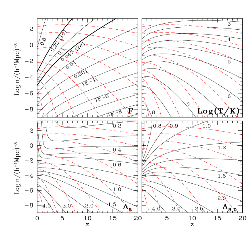
Figure 2: The comoving number density of dark matter haloes with mass exceeding $M(z)$ is plotted as a function of redshift for the standard $\rm\Lambda CDM$ model, $\Omega_{\rm m,0}=0.3$, $\Omega_{\rm\Lambda,0}=0.7$, $h=0.7$ and $\sigma_{8}=0.9$, and for various definitions of the limiting mass $M(z)$. In the panel at top left, solid lines show the halo abundance when $M(z)$ is chosen to define haloes containing a given fraction $F$ of all cosmic matter; the values of $F$ are given as labels against each curve. The particular values of $F$ corresponding to “$1\sigma$” (or $M_{*}$) and “$2\sigma$” haloes are noted. The panel at top right shows results when $M(z)$ is chosen to correspond to a given virial temperature at each redshift; labels correspond to the logarithm of the temperature in Kelvin. For the panel at bottom left, the limiting mass $M(z)$ is chosen so that the comoving clustering length of haloes (as measured by $\Delta_{8}$) has a given value, shown by the label on each solid curve. Finally, for the panel at bottom right, $M(z)$ is chosen so that the clustering strength of the halo descendants at $z=0$ (as measured by $\Delta_{8,0}$) has a given value listed by the label on each curve. In all these plots, dashed lines repeat the curves of Figure 1 and so can be used to assign a limiting mass $M(z)$ to each point in the abundance-redshift plane.

In this section we plot the halo abundances predicted by the analytic formulae given above for a version of the current “concordance” $\Lambda$CDM model. Specifically we pick a model with $\Omega_{\rm m,0}=0.3$, $\Omega_{\rm\Lambda,0}=0.7$, $h=0.7$ and $\sigma_{8}=0.9$. We have chosen to show comoving abundance as a function of redshift for haloes with masses exceeding $M(z)$ for various definitions of the mass limit $M(z)$. We have found these plots to be particularly instructive, and by comparing them it is possible to read off a wide variety of halo properties as a function of redshift. In the following we will consider halo abundance as a function of halo mass, of total halo contribution to the cosmic density, of halo virial temperature, of halo clustering strength, and of the clustering strength of the present-day descendants of high redshift haloes.

3.1 Halo abundance as a function of mass

In Figure 1 we show the comoving abundance of haloes of given mass as a function of redshift for a wide range of halo masses. Plots of this kind have appeared before in the literature a number of times (e.g. Efstathiou & Rees 1988; Cole & Kaiser 1989). Our figure updates earlier versions in that it is appropriate for the currently popular model and it uses more accurate formulae (equation 14) than the Press-Schechter model used by previous authors. It is also required for comparison with the other plots we discuss below.

Figure 1 illustrates a number of well known properties of the standard $\Lambda$CDM model. Haloes as massive as a rich galaxy cluster like Coma ($M\sim 10^{15}\,\rm M_{\odot}$) have an average spacing of about $100h^{-1}$Mpc today, but their abundance drops dramatically in the relatively recent past. By $z=1.5$ it is already down by a factor exceeding 1000, corresponding to a handful of objects in the observable Universe. The decline in the abundance of haloes with mass similar to that of the Milky Way ($M\sim 10^{12}\,\rm M_{\odot}$) is much more gentle. By $z=5$ the drop is only about one order of magnitude. At the smallest masses shown ($M\sim 10^{7}$ to $10^{8}\,\rm M_{\odot}$) there is little change in abundance over the full redshift range $0<z<20$ that we plot. Notice also that the abundance of such low mass haloes is actually declining slowly at low redshifts as members of these populations merge into larger systems faster than new members are formed. It is interesting that haloes of mass $10^{9}\,\rm M_{\odot}$ are as abundant at $z=20$ as $L_{*}$ galaxies are today, and haloes of $10^{10}\,\rm M_{\odot}$ are as abundant as present-day rich galaxy clusters. Thus a significant population of relatively massive objects could, in principle, be present even at these early times.

3.2 The cosmic mass fraction in massive haloes

For the upper left plot of Figure 2 we have used equation (15) to compute lower mass limits $M(z)$ such that the halo population contains a given fixed fraction of all cosmic mass. As noted in Section 2, for our “improved” Press-Schechter models haloes corresponding to $>1\sigma$ and $>2\sigma$ initial fluctuations contain 0.22 and 0.047 of the cosmic mass respectively, independent of redshift. By our conventions, the $1\sigma$ limiting mass is defined as $M_{*}$, the characteristic mass of clustering. By comparing the $1\sigma$ line in Figure 2 with the constant mass lines copied over from Figure 1, one can see that $M_{*}$ drops from just over $10^{13}\,\rm M_{\odot}$ at the present day to just below $10^{7}\,\rm M_{\odot}$ at $z=6$.

From the redshift zero axis on this same plot, we can see that one percent of all mass today is in objects more massive than $10^{15}\,\rm M_{\odot}$, ten percent is in objects more massive than $10^{14}\,\rm M_{\odot}$, but more than half is in objects less massive than $10^{10}\,\rm M_{\odot}$, one percent of the halo mass of the Milky Way. According to our standard model, the mass of the Universe is currently distributed over objects with an extremely wide range of masses. The predicted distribution of the lower half of the mass is actually very uncertain, since use of our formulae in this regime would involve extrapolation far below the limits for which they have been tested against $N$-body simulations (see Jenkins et al. 2001). For this reason we do not give curves for mass fractions above 0.5.

At redshift 5 just under one percent of all matter is in haloes more massive than that of the Milky Way, but by redshift 10 this fraction has dropped to $10^{-6}$. At redshift 10 there is, nevertheless, still one percent of all matter in haloes more massive than about $10^{10}\,\rm M_{\odot}$ and five percent in haloes more massive than about $10^{8}\,\rm M_{\odot}$. By redshift 20 only about $10^{-3}$ of all matter is in haloes more massive than $10^{8}\,\rm M_{\odot}$ and only about $10^{-6}$ in haloes more massive than $10^{10}\,\rm M_{\odot}$.

3.3 Halo abundance as a function of temperature

Because we define the boundary of our haloes at fixed overdensity relative to the cosmic mean, the mass we assign to a given dark halo will vary with redshift even in the absence of evolution. This is actually quite a strong effect. For example, we would assign an order of magnitude smaller mass to a halo like the Milky Way’s at redshift 5 than at the present day, even if its density profile was unchanged. As a result, and also because both the ionisation and the cooling of diffuse gas within a halo depend primarily on its temperature, it is often more helpful to study the abundance of haloes as a function of characteristic temperature (or equivalently of characteristic circular velocity) rather than of mass. We give the relationship between these quantities in equations (1) and (4) above, and we compare the evolution of halo abundance at fixed temperature to that at fixed mass in the upper right panel of Figure 2. Again, we are not the first to make such abundance evolution plots, but the current plots update earlier versions by using more accurate formulae and the current “best bet” cosmological parameters.

The first point to note from this diagram is that made above – haloes of a given temperature correspond to different masses at different redshifts. Thus a $10^{6}$K halo (with $V_{c}\sim 200$km/s) has a mass of about $2\times 10^{12}\,\rm M_{\odot}$ at the present day, but a mass of only $2\times 10^{10}\,\rm M_{\odot}$ at $z=20$. Conversely, a $2\times 10^{10}\,\rm M_{\odot}$ halo at $z=0$ has a temperature of only $5\times 10^{4}$K and so a circular velocity of only 36 km/s.

A second important point is that over a wide range of temperature the evolution of abundance with redshift is quite slow. Thus the abundance of haloes hotter than 1keV is approximately the same at $z=3$ as at $z=0$. Indeed, for temperature limits equal to or below the observed temperatures of Abell clusters ($T\la 5$keV) the abundance of objects actually increases with increasing redshift away from $z=0$. An X-ray temperature-selected sample of galaxy clusters is expected to show little abundance evolution unless the temperature threshold for inclusion is quite high. For the characteristic temperature of the Milky Way’s halo, $T\sim 10^{6}$K corresponding to $V_{c}\sim 200$km/s, the abundance of systems at $z=8$ is about the same as it is at $z=0$. Apparently the formation of galaxies like our own could, in principle, start at very early times.

Infall onto haloes with characteristic temperatures greater than $10^{4}$K will produce strong enough shocks to ionise the infalling gas. As a result, atomic line cooling is expected to be efficient in such systems and to lead to condensation of dense gas at their centres, possibly with associated star formation. Figure 2 shows the abundance of such systems to be almost constant at $n\sim 10h^{3}$Mpc^-3 all the way from $z=20$ down to $z=3$. At $z=15$ about 1% of all matter is already in objects above the collisional ionization threshold, and by $z=5$ this fraction has climbed to about 20%. In the absence of effects other than cooling, roughly 1 and 20% of all baryons would be in dense systems by redshifts of 15 and 5 respectively, whereas current estimates suggest that this fraction is below 10% even at $z=0$ (Balogh et al. 2001). In fact, it has long been argued that radiative and hydrodynamic feedback must be associated with the formation of stars and active galactic nuclei, and that it must limit the condensation of gas within smaller haloes (White & Rees 1978; White & Frenk 1991; Efstathiou 1992).

According to the calculations of Gnedin (2000) for standard reionisation models, haloes with $T\la 10^{5}{\,\rm K}$ are unable to trap, and therefore to cool, significant amounts of diffuse photoionised gas at low redshifts ($z\la 5$). Since reionisation is known to have occurred before $z=6$, Figure 2 suggests that more than half of all baryons were never part of a halo in which cooling was efficient. These baryons must currently reside in a diffuse intergalactic medium (see Cen & Ostriker 1999).

3.4 Halo clustering

As noted in Section 2 we have decided to characterise the clustering of haloes as a function of mass and redshift using $\Delta_{8}(M,z)$ the rms overdensity in the number of haloes more massive than $M$ at redshift $z$ after smoothing with a spherical top-hat filter of comoving radius $8h^{-1}$Mpc. This measure is convenient to calculate and has become traditional because it is close to unity for moderately bright galaxies in the present Universe. The theory of Mo & White (1996), as corrected empirically by Jing (1998) and Sheth & Tormen (1999), shows that at each redshift and for halo masses below $M_{*}$, the value of $\Delta_{8}(M,z)$ varies little with $M$ and is just below $D(z)\sigma_{8}$, the corresponding mass density fluctuation. For halo masses above $M_{*}(z)$ the value of $\Delta_{8}$ increases rapidly with $M$ [see equations (19) and (21)].

The lower left panel of Figure 2 shows the abundance-redshift relation for haloes more massive than $M(z)$ chosen so that $\Delta_{8}$ takes specific values, given as labels beside each curve. From the $y$-axis of this plot we see that no halo population in the present Universe has $\Delta_{8}<0.5$, that haloes more massive than $M_{*}$ currently have $\Delta_{8}\sim 1.2$, and that rich galaxy clusters at $z=0$ have $\Delta_{8}\ga 3$. The locus of $M_{*}$ haloes is clearly visible in this plot joining the points of maximum curvature on each of the constant $\Delta_{8}$ curves. (Compare with the $1\sigma$ curve in the upper left panel of Figure 2.)

A striking feature of this clustering plot is the weak dependence of clustering strength on redshift for haloes more massive than $M_{*}(z)$. In this regime the increase in bias with increasing redshift compensates for the decreasing clustering strength of the underlying mass distribution. Thus haloes with the abundance of $L_{*}$ galaxies, $n\sim 10^{-3}h^{3}{\rm Mpc}^{-3}$, have $\Delta_{8}\sim 0.9$ for all $z<10$. Over this redshift range their mass drops from about $10^{13}\,\rm M_{\odot}$ at $z=0$ to about $10^{11}\,\rm M_{\odot}$ at $z=10$. It is interesting that their clustering strength is close to that measured at $z\sim 3$ for the “Lyman break” galaxy population identified by Steidel et al (1996; see also Adelberger et al. 1998) which indeed has a comoving number density of about $0.001h^{3}{\rm Mpc}^{-3}$. This has led many authors, beginning with Mo & Fukugita (1996), to speculate that Lyman break galaxies may be the central objects of $z\sim 3$ haloes and that their UV luminosity may correlate well with their halo mass. The halo mass of a Lyman break galaxy at $z\sim 3$ can then be read off from Figure 2; it is $M\sim 10^{12}\,\rm M_{\odot}$. Clearly a more detailed study of the clustering of high redshift galaxies should provide detailed information about how the masses of the haloes they inhabit are related to their observable properties (Baugh et al. 1998; Mo, Mao & White 1999; Somerville, Primack & Faber 2001; Wechsler et al 2001; Shu, Mao & Mo 2001).

Another surprising property of the clustering predictions is that haloes of given mass actually become more strongly clustered with increasing redshift once the mass chosen exceeds $M_{*}(z)$. The same is also true, although more weakly so, for samples selected to a fixed virial temperature. Thus galaxy clusters selected to a fixed rest-frame X-ray temperature limit are expected to be equally clustered at $z=1$ and at $z=0$, while clusters selected to a given observed temperature limit will be substantially more clustered at the higher redshift. Relatively low mass haloes can be surprisingly strongly clustered even at very high redshift. For example, at $z=20$ haloes of mass above $10^{8}\,\rm M_{\odot}$ have a virial temperature above $2\times 10^{4}$K, contain 0.1% of all matter, and have a clustering strength of $\Delta_{8}\sim 0.4$.

3.5 Clustering of the present-day remnants of high redshift haloes

One of the major puzzles in current astrophysics is the relation between the objects observed in the high redshift Universe and those around us today. Which present-day galaxies contain the stellar population we see forming in Lyman break galaxies? Which host the massive black holes which powered high redshift quasars? Where are the remnants of the very first stellar populations? How are the heavy elements they produced distributed through the present Universe? Our current understanding of where to look for such remnants comes primarily from simulations (Governato et al 1998; Cen & Ostriker 1999; White & Springel 2000; Kauffmann & Haehnelt 2001) but considerable intuition can also be gained from simpler analytic estimates of remnant clustering (Mo & Fukugita 1996). We illustrate this here using $\Delta_{8,0}(M,z)$, the clustering strength of the present-day descendants of halos with mass greater than $M$ at redshift $z$. Note that this measure weights each descendant by the number of its high redshift progenitors.

In the lower right panel of Figure 2 we give abundance-redshift relations for haloes selected to mass limits $M(z)$ which give the specific values of $\Delta_{8,0}$ listed against each curve. Along the $z=0$ axis the abundance-clustering strength relation in this plot is, of course, identical to that of the $\Delta_{8}$ plot in the lower left panel. At higher redshifts $\Delta_{8,0}$ exceeds $\Delta_{8}$ everywhere as a result of the growth of clustering with time. The $\Delta_{8,0}=0.9$ curve is close to the curve for $F=0.22$ in the top left panel; at each redshift $1\sigma$ haloes are unbiased relative to the mass, and their descendants remain unbiased as clustering evolves. Over most of our abundance-redshift plot, $\Delta_{8,0}$ is substantially larger than 0.9, so that the the remnants of the relevant halo populations are more clustered today than the dark matter or than $L_{*}$ galaxies. The descendants of $z=3$ halos with the abundance of Lyman break galaxies ($n\sim 10^{-3}h^{3}{\rm Mpc}^{-3}$) have $\Delta_{8,0}\sim 1.6$, suggesting that the Lyman break systems have evolved preferentially into massive early-type galaxies (Mo & Fukugita 1996; Governato et al. 1998).

Bright quasars have now been seen to redshifts beyond 6. Their observed comoving number density is $n\sim 4\times 10^{-8}h^{3}{\rm Mpc}^{-3}$ at $z\sim 3$, and $n\sim 2\times 10^{-9}h^{3}{\rm Mpc}^{-3}$ at $z\sim 6$ (Fan et al. 2001). If we adopt a typical quasar lifetime at redshift $z$ of $3\times 10^{7}[H_{0}/H(z)]$ years (e.g. Kauffmann & Haehnelt 2000), the implied number density of host haloes is $n\sim 10^{-5}h^{3}{\rm Mpc}^{-3}$ at $z\sim 3$, and $n\sim 10^{-6.5}h^{3}{\rm Mpc}^{-3}$ at $z\sim 6$. From Figure 1 we see that the masses of such haloes are $M\sim 10^{13}\,\rm M_{\odot}$, suggesting there will be no problem forming such luminous objects by the observed redshifts in our standard cosmology. At $z\sim 3$ these haloes have correlation strength $\Delta_{8}\sim 1.5$ corresponding to a comoving correlation length of about $8\,h^{-1}{\rm{Mpc}}$ . Their present-day descendants then have $\Delta_{8,0}\sim 2$, or a correlation length about $11\,h^{-1}{\rm{Mpc}}$. The predicted correlation lengths for the $z\sim 6$ quasars and their descendants are about $11\,h^{-1}{\rm{Mpc}}$ and $14\,h^{-1}{\rm{Mpc}}$ respectively. These $z=0$ correlation lengths are comparable to those of the most luminous elliptical galaxies in the present Universe. Such galaxies are indeed now thought to host the $\sim 10^{9}\,\rm M_{\odot}$ black holes which must have powered these distant quasars (Gebhardt et al 2000; Ferrarese & Merritt 2000). Notice that our inferred clustering lengths are quite sensitive to the quasar lifetimes we assumed. A number of authors have pointed out that clustering can therefore constrain quasar lifetimes (La Franca, Andreani & Cristiani 1998; Fang & Jing 1998; Haehnelt, Natarajan & Rees 1998; Haiman & Hui 2001; Martini & Weinberg 2001; Kauffmann & Haehnelt 2001).

High-$z$ quasars are also expected to be strongly correlated with other objects at the same redshift. For example, at $z\sim 6$ the mean density enhancement of haloes with $M\sim 10^{10}\,\rm M_{\odot}$ in an $8\,h^{-1}{\rm{Mpc}}$ sphere surrounding a bright quasar is the product of the $\Delta_{8}$ values for the two populations, i.e. about $0.4\times 2=0.8$. Such dense environments surrounding quasars may have important implications for the interpretation of quasar absorption spectra, in particular for the proximity effect or for the effective absorption optical depth of the foreground IGM.

As a final example of these clustering plots, we consider the distribution of the metals produced by the first generations of stars. Tegmark et al. (1997, see also Loeb & Barkana 2001 and references therein) showed that primordial gas in haloes with virial temperatures above $3\times 10^{3}{\,\rm K}$ can cool by molecular hydrogen and atomic line cooling at $z\la 20$. Population III stars may form in such haloes, which would then begin ionising the intergalactic medium and polluting it with heavy elements. As one can see from Figure 2, just below 1 percent of the cosmic mass is already in such haloes at $z\sim 20$, and their clustering is already moderately strong, $\Delta_{8}\sim 0.25$. By redshift zero the metals produced by this population will have $\Delta_{8,0}\sim 1.15$ and so will be as clustered as $L_{*}$ galaxies. By redshift 3 the clustering strength of these metals has already reached $\Delta_{8}\sim 0.6$. Thus the metallicity distribution in the gas probed by observed Lyman $\alpha$ forest is predicted to be highly inhomogeneous even if enrichment is due to Population III objects burning at early times. [These various clustering strengths can be read off Figure 2 as follows. The upper left panel gives $n\sim 10^{2}h^{3}{\rm Mpc}^{-3}$ as the abundance of objects at $z=20$ with a virial temperature above $3\times 10^{3}$K. The panels at lower left and lower right then give the clustering strength of these objects and of their $z=0$ descendants respectively. The clustering strength of the $z=3$ descendants is obtained by following the $\Delta_{8,0}=1.15$ line in the bottom left panel from $z=20$ down to $z=3$ where it corresponds to $n\sim 10^{-1.5}h^{3}{\rm Mpc}^{-3}$. The appropriate clustering strength $\Delta_{8}\sim 0.6$ is then read off from the bottom left panel.]

4 Concluding words

Throughout this paper we have discussed a single version of the current standard $\Lambda$CDM model, but the formulae given in Section 2 are complete enough that the reader can easily produce modified versions of our plots for other choices of the cosmological parameters. These can be useful for understanding whether the abundance and clustering of a population of interest may be sensitive to the particular cosmological context in which it is evolving. We have given examples of applications to galaxy clusters, to Lyman break galaxies, to quasars, and to the enrichment of the intergalactic gas by high redshift Population III stars. Other applications are possible, but these already illustrate how the observed abundance and clustering of a population can be used to infer the masses of the dark haloes in which it is embedded. Even for the “standard” model we have studied, a number of the properties evident from our plots seem at first sight to be counter-intuitive or surprising. We have found this graphical presentation of the model properties to be surprisingly useful, and we hope that others will also.

References

- [1]
- [2] Adelberger K.L., Steidel C.C., Giavalisco M., Pettini M., Kellogg M., 1998, ApJ, 505, 18
- [3] Balogh M.L., Pearce F.R., Bower R.G., Kay S.T., 2001, MNRAS, 326, 1228
- [4] Bardeen J.M., Bond J.R., Kaiser N., Szalay A.S., 1986, ApJ, 304, 15
- [5] Baugh C.M., Cole S., Frenk C.S., Lacey C.G., 1998, ApJ, 498, 504
- [6] Bennett C.L., et al., 1996, ApJL, 464, 1
- [7] Benson A.J., Baugh C.M., Cole S., Frenk C.S., Lacey C.G., 2000, MNRAS, 316, 107
- [8] Blumenthal G.R., Faber S.M., Primack J.R., Rees M.J., 1984, Nat, 311, 517
- [9] Bond J.R., Cole S., Efstathiou G., Kaiser N., 1991, ApJ, 379, 440
- [10] Carroll S.M., Press W.H., Turner Edwin L., 1992, ARA&A, 30, 499
- [11] Casas-Miranda R., Mo H.J., Sheth R.K., Börner G., 2002, MNRAS, in press
- [12] Cen R., Ostriker J.P., 1999, ApJ, 519, L109
- [13] Cole S., Kaiser N., 1989, MNRAS, 237, 1127
- [14] Croft R.A.C., Weinberg D.H., Pettini M., Hernquist L., Katz N., 1999, ApJ, 520, 1
- [15] Davis M., Efstathiou G., Frenk C.S., White S.D.M., 1985, ApJ, 292, 371
- [16] de Bernardis P., et al., 2002, ApJ, 564, 559
- [17] Efstathiou G., 1992, MNRAS, 256, P43
- [18] Efstathiou G., Rees M.J., 1988, MNRAS, 230, P5
- [19] Efstathiou G., et al., 2002, MNRAS, 330, L29
- [20] Fan X.H. et al. 2001, AJ, 122, 2833
- [21] Fang L.-Z., Jing Y.P., 1998, ApJ, 502, L95
- [22] Ferrarese L., Merritt D., 2000, ApJ, 539, L9
- [23] Freedman W., et al., 2001, ApJ, 553, 47
- [24] Gebhardt K., et al., 2000, ApJ, 543, L5
- [25] Gnedin N.Y., 2000, ApJ, 542, 535
- [26] Governato F., Baugh C.M., Frenk C.S., Cole S., Lacey C.G., Quinn T., Stadel J., 1998, Nat, 392, 359
- [27] Guth A., 1997, The Inflationary Universe, The Quest for a New Theory of Cosmic Origins. Addison-Wesley, Reading
- [28] a value of Haehnelt Martin G., Natarajan P., Rees M.J., 1998, MNRAS, 300, 817
- [29] Haiman Z., Hui L., 2001, 2001, ApJ, 547, 27
- [30] Hjorth J., Burud I., Jaunsen A.O., Schechter P.L., Kneib J.P., Andersen M.I., Korhonen H., Clasen J.W., Kaas A.A., Ostensen R., Pelt J., Pijpers F.P., 2002, ApJ Lett., in press
- [31] Jenkins A., Frenk C.S., White S.D.M., Colberg J.M., Cole S., Evrard A.E., Couchman H.M.P., Yoshida N., 2001, MNRAS, 321, 372
- [32] Jing Y.P., 1998, ApJ, 503, L9
- [33] Jing Y.P., Mo H.J., Boerner G., 1998, ApJ, 494, 1
- [34] Kauffmann G., Haehnelt M., 2000, MNRAS, 311, 576
- [35] Kauffmann G., Haehnelt M., 2001, astro-ph/0108275
- [36] La Franca F., Andreani P., Cristiani S., 1998, ApJ, 497, 529
- [37] Loeb A., Barkana R., 2001, ARA&A, 39, 19
- [38] Martini P., Weinberg D.H., 2001, ApJ, 547, 12
- [39] Mo H.J., Fukugita M., 1996, ApJ, 467, L9
- [40] Mo H.J., Jing Y.P., White S.D.M., 1996, MNRAS, 282, 1096
- [41] Mo H.J., Mao S., White S.D.M., 1999, MNRAS, 304, 175
- [42] Mo H.J., White S.D.M., 1996, MNRAS, 282, 347
- [43] Olive K.A., Steigman G., Walker T.P., 2000, Phys. Rep., 333, 389
- [44] O’Meara J.M., Tytler D., Kirkman D., Suzuki N., Prochaska J. X., Lubin D., Wolfe A.M., 2001, ApJ, 552, 718
- [45] Peacock J.A., et al. 2001, Nat, 410, 169
- [46] Peebles P.J.E. 1982, ApJ, 263, L1
- [47] Press W.H., Schechter P., 1974, ApJ, 187, 425 (PS)
- [48] Perlmutter S., et al. 1999, ApJ, 517, 565
- [49] Reiprich T.H., Böhringer H., 2002, ApJ, 567, 716
- [50] Schuecker P., et al., 2001, A&A, 368, 86
- [51] Seljak U., 2001, preprint (astro-ph/0111362)
- [52] Sheth R.K., Tormen G., 1999, MNRAS, 308, 119
- [53] Sheth R.K., Tormen G., 2002, MNRAS, 329, 61
- [54] Sheth R.K., Mo H.J., Tormen G., 2001, 2001, MNRAS, 323, 1
- [55] Shu, C.G., Mao S.D., Mo H.J., 2001, MNRAS, 327, 895
- [56] Somerville R.S., Primack J.R., Faber S.M., 2001, MNRAS, 320, 504
- [57] Steidel C.C., Giavalisco M., Pettini M., Dickinson M., Adelberger K.L., 1996, ApJ, 462, L17
- [58] Tegmark M., Silk J., Rees M.J., Blanchard A., Abel T., Palla F., 1997, ApJ, 474, 1
- [59] Viana P.T.P., Liddle A.R., 1999, MNRAS, 303, 535
- [60] Viana P.T.P., Nichol R.C., Liddle A.R., 2002, ApJ, 569, L75
- [61] Van Waerbeke L., et al., 2001, A&A, 374, 757
- [62] Wechsler R.H., Somerville R.S., Bullock J.S., Kolatt T.S., Primack J.R., Blumenthal G.R., Dekel A., 2001, ApJ, 554, 85
- [63] White S.D.M., Efstathiou G., Frenk C.S., 1993, MNRAS, 262, 1023
- [64] White S.D.M., Frenk C.S., 1991, ApJ, 379, 52
- [65] White S.D.M., Rees, M., 1978, MNRAS, 183, 341
- [66] White S.D.M., Springel V., 2000, In A. Weiss, et al. eds. The First Stars, Springer: Berlin, p.327