Low power BL Lacertae objects and the blazar sequence

The spectral properties of blazars seem to follow a phenomenological sequence according to the source luminosity. By inferring the source physical parameters through (necessarily) modeling the blazar spectra, we have previously proposed that the sequence arises because the particles responsible for most of the emission suffer increasing radiative losses as the luminosity increases. Here we extend those results by considering the widest possible range of blazar spectral properties. We find a new important ingredient for shaping the spectra of the lowest power objects, namely the role of a finite timescale for the injection of relativistic particles. Only high energy particles radiatively cool in such timescale leading to a break in the particle distribution: particles with this break energy are those emitting most of the power, and this gives raise to a link between blazar spectra and total energy density inside the source, which controls the cooling timescale. The emerging picture requires two phases for the particle acceleration: a first pre–heating phase in which particles reach a characteristic energy as the result of balancing heating and radiative cooling, and a more rapid acceleration phase which further accelerate these particles to form a power law distribution. While in agreement with standard shock theory, this scenario also agrees with the idea that the luminosity of blazars is produced through internal shocks, which naturally lead to shocks lasting for a finite time.

1 Introduction

Blazars appear to come in different flavors, according to e.g. their strong or weak (or even absent) broad emission lines, their optical polarization and the position of the peak of the synchrotron component in their spectral energy distribution (SED), namely at low (mm–IR) or high (UV and soft X–ray) frequencies (e.g. Padovani & Urry 2001). The latter criterion has been indeed (proposed and) favored in the last few years as possibly associated with more ‘physical’ and fundamental properties of the sources (Giommi & Padovani 1994; Fossati et al. 1998, hereafter F98; Ghisellini et al. 1998, hereafter G98). In particular, within this scenario, F98 and G98 proposed that the different sub–classes of blazars form a spectral and physical sequence in the position and intensity of the peaks, controlled primarily by one parameter, which they identified with the bolometric observed luminosity. The sequence in the SED has been described by F98 phenomenologically (on the assumption that the bolometric luminosity scales linearly with the radio one), while G98 modeled the SED of individual blazars adopting a homogeneous synchrotron plus inverse Compton model.

In this way G98 deduced values of the physical quantities behind the sequence, i.e. translated the spectral trend (power vs SED) into a trend between physical parameters, which could be consistently interpreted as governed by the importance of radiative cooling. In fact they found an inverse correlation between the energy of the particles emitting at the peaks of the SED, $\gamma_{\rm peak}m_{\rm e}c^{2}$, and the energy density $U$ (magnetic and radiation fields) as seen in the frame comoving with the emitting plasma. More specifically the correlation appeared to be well approximated by $\gamma_{\rm peak}\propto U^{-0.6}$, directly implying that the radiative cooling rate at $\gamma_{\rm peak}$ ($\propto\gamma^{2}_{\rm peak}U$) is almost constant for all sources, suggesting a key role of the radiative cooling process in shaping the SED.

Given the potential relevance of such result in the attempt to understand the dissipation and particle acceleration mechanisms, we decided to further explore the presence of such a trend over a larger range of the parameter space. In fact, in order to efficiently constrain the model parameters (in particular from the high emission component) the modeling procedure in G98 was applied only to those sources detected in the $\gamma$-ray band by EGRET (the high energy instrument onboard the Compton Gamma Ray Observatory), for which both the $\gamma$–ray spectral shape and the cosmological distance were determined.

As the majority of the EGRET detected blazars comprises sources of large power, Flat Spectrum Radio Quasars (FSRQ) and Low energy peak BL Lacs (LBLs, in the definition of Giommi & Padovani 1995), such initial selection of the sources was biased against low power BL Lacs, under–represented in G98, and thus against sources with high energy peaks at very high frequencies (above the EGRET range).

In reality a few of those sources have been detected by Cherenkov telescopes in the TeV band and the modeling of their broad band energy distribution confirmed the phenomenological trend between the SED and the source power (F98). Furthermore a number of low power BL Lacs have been recently observed by $Beppo$SAX and detected in the X–ray band up to $\sim$ 100 keV. Therefore there is now a reasonable number of comparatively weak sources with sufficient data to constrain the shape of their SED and thus explore the $\gamma_{\rm peak}$–$U$ correlation at high $\gamma_{\rm peak}$ (low $U$).

Such an extension becomes even more relevant since a change in the correlation is indeed expected. In fact we already stress here that it is possible to immediately predict a deviation from the $\gamma_{\rm peak}\propto U^{-0.6}$ behavior. Consider for illustration the case of the most extreme sources, e.g. Mkn 501 in the flaring state and 1ES 1426+428 (Pian et al. 1998; Costamante et al. 2001). They are both TeV detected sources (Catanese & Weekes 1999 and references therein; Horan 2000, Djannati–Atai, priv. comm.) and also showed a synchrotron component peaking above $\sim$ 100 keV. The peak at TeV energies implies that $\gamma_{\rm peak}$ exceeds $10^{5}$–$10^{6}$: according to the correlation found by G98 this would correspond to magnetic fields weaker than $\sim$ 0.05 G. However this implies a synchrotron peak frequency two–three orders of magnitude smaller than observed. We therefore expect a change in the correlation at the high $\gamma_{\rm peak}$ end of the parameter space, and so plausibly we expect to find an additional key ingredient, besides radiative cooling, regulating the blazar SED.

In this paper we thus explore such issue by extending the sample of blazars, including several extreme high energy peakers, as presented in Section 2. We then consider at first the modeling of the SED of such objects with the synchrotron inverse Compton model used by G98 and examine the results in relation to the $\gamma_{\rm peak}$–$U$ correlation in Section 3. The parameters inferred from the modeling imply that in the extreme sources it is necessary to consider the effect of the duration of the relativistic particle injection as this can be comparable or shorter than the relevant cooling timescale (see also Sikora et al. 2001, Sikora & Madejski 2001). Therefore in Section 4 we re–analyze the whole sample of blazars with a finite injection time model, discuss the findings and propose a physical interpretation for the $\gamma_{\rm peak}$–$U$ relation. Summary and conclusions are reported in Section 5.

2 The extreme BL Lac objects

We consider “extreme BL Lac objects” the sources with a synchrotron peak at energies exceeding 0.1 keV. The frequency of the peak, $\nu_{\rm peak}$, can be thus directly determined by broad band X–ray detectors, such as those onboard the BeppoSAX satellite.

Candidate extreme BL Lacs were selected by Costamante et al. (2001) on the basis of their SEDs and their broad band (radio/optical/X–rays) spectral indices, which constitute good indicators of the location of the synchrotron peak, as objects of different characteristics tend to gather in different regions of the spectral index parameter spaces (Stocke et al. 1991; Padovani & Giommi 1995; F98). For five out of the seven objects observed by BeppoSAX (Costamante et al. 2001) $\nu_{\rm peak}$ turned out to be indeed in the X–ray range and for one of them, 1426+428, $\nu_{\rm peak}$ was bound to be at frequencies larger than 100 keV, as occurred in Mkn 501 during the flaring state of 1997 (Pian et al. 1998) and in 1ES 2344+514 (Giommi, Padovani & Perlman 2000). These three, so far unique, sources have all been detected at TeV energies. In addition to these, here we also reconsider Mkn 501 and 1ES 2344+514, together with Mkn 421, for modeling their SED observed during flaring states (the SED in G98 corresponded only to the more “quiescent” states) and include in the sample PKS 2005–489 and 1ES 1101–232, since BeppoSAX observations of these sources revealed a high peak synchrotron frequency (Wolter et al. 2000; Tagliaferri et al. 2001).

In order to extend the range covered by the $\gamma$–$U$ relation we also considered, at the other end of the blazar sequence, three very powerful FSRQ recently found at high redshift (Fabian et al. 2001a,b; Moran & Helfand 1997 and references therein). In fact, although they do not have a complete information on their high energy peak (not being detected by EGRET), their hard X–ray spectra constrain the emission model rather tightly.

In Table 1 we list the sources included in this paper (and not already present in the sample of G98) and the references to the data used in constructing the SEDs shown in Fig. 1a,b,c.

Source	Other name	$z$	Ref
0033$+$595	1ES	0.086a	NED, Co01, Pe96, SG99, Br97
0120$+$340	1ES	0.272	NED, Co01, BS94
0548$-$322	1ES, PKS	0.069	NED, Co01, GAM95, Pe96, WW90, Ta95, Ti94
1101$-$232	1ES	0.186	NED, Wo00, SG99
1101$+$384	Mkn 421	0.031	NED, Ma95, Ma96, Sc97
1114$+$203	RGB J1117+202	0.139b	NED, Co01, Br97
1218$+$304	1ES	0.130	NED, Co01, GAM95, Pi93, Sa94, Fo98
1426$+$428	1ES	0.129	NED, Co01, GAM95, La96, Sa93, Sa97, Fi94, Ho00
1652$+$398	Mkn 501	0.034	NED, Pi98
2005$-$489	PKS	0.071	NED, Ta01
2344$+$514	1ES	0.044	NED, Gi00, SG99, Pe96, Fi94
2356$-$309	H 2356–309	0.165	NED, Co01, Be92, Fa94
0525$-$334	PMN	4.41	Fa01a
1428$+$422	B3	4.715	Fa01b
1508$+$571	GB	4.301	MH97

Table 1: List of the sources studied in this paper. The line separates the extreme BL Lacs (above) and the very powerful FSRQ (below). a) Tentative, Perlman, priv. comm. as reported in Falomo & Kotilanen 1999. b) redshift reported in Bohringer et al. 2000. Sources of data: Be92: Bersanelli et al. 1992; Br97: Brinkmann et al. 1997; BS94: Brinkmann & Siebert 1994; Co01: Costamante et al. 2001; F98: Fossati et al. 1998; Fa01a: Fabian et al. 2001a; Fa01b: Fabian et al. 2001b; Fa94: Falomo et al. 1994; Fi94: Fichtel et al. 1994; GAM95: Giommi, Ansari & Micol 1991; Gi00: Giommi, Padovani & Perlman 2000; Ho00: Horan 2000; La96: Lamer, Brunner & Staubert 1996; Ma95: Macomb et al. 1995; Ma96: Macomb et al. 1996; MH97: Moran & Helfand 1997; Pe96: Perlman et al. 1996; Pi93: Pian & Treves 1993; Pi98: Pian et al. 1998 (and references therein); Sa93: Sambruna et al. 1993; Sa94: Sambruna et al. 1994; Sa97: Sambruna et al. 1997; Sc97: Schubnell 1997; SG99: Stevens & Gear 1999; Ta95: Tashiro et al. 1995; Ta01: Tagliaferri et al. 2001 (and references therein); Wo00: Wolter et al. 2000; WW90: Worral & Wilkes 1990.

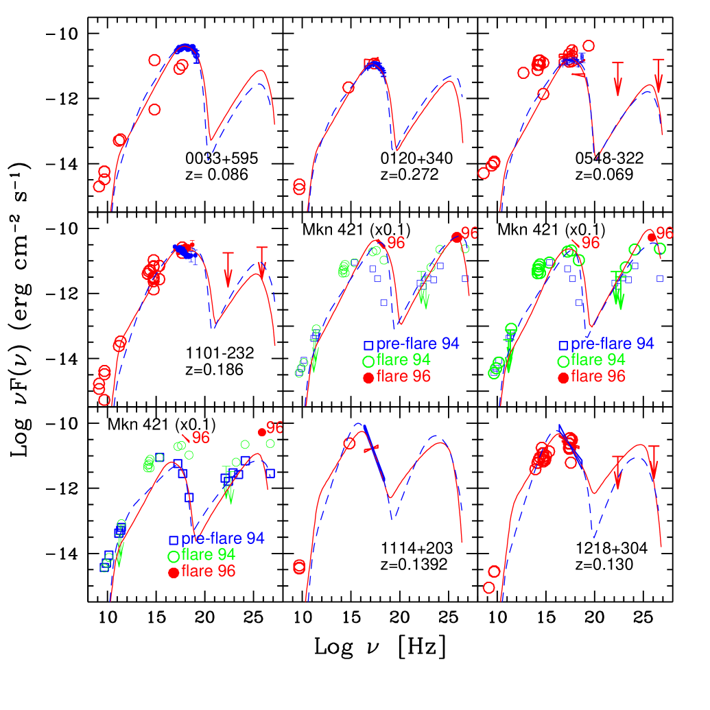
Figure 1: a): The SED of our extreme BL Lac objects. The solid and dashed lines correspond to the steady–state and finite injection time models, as discussed in Section 3 and 4, respectively.

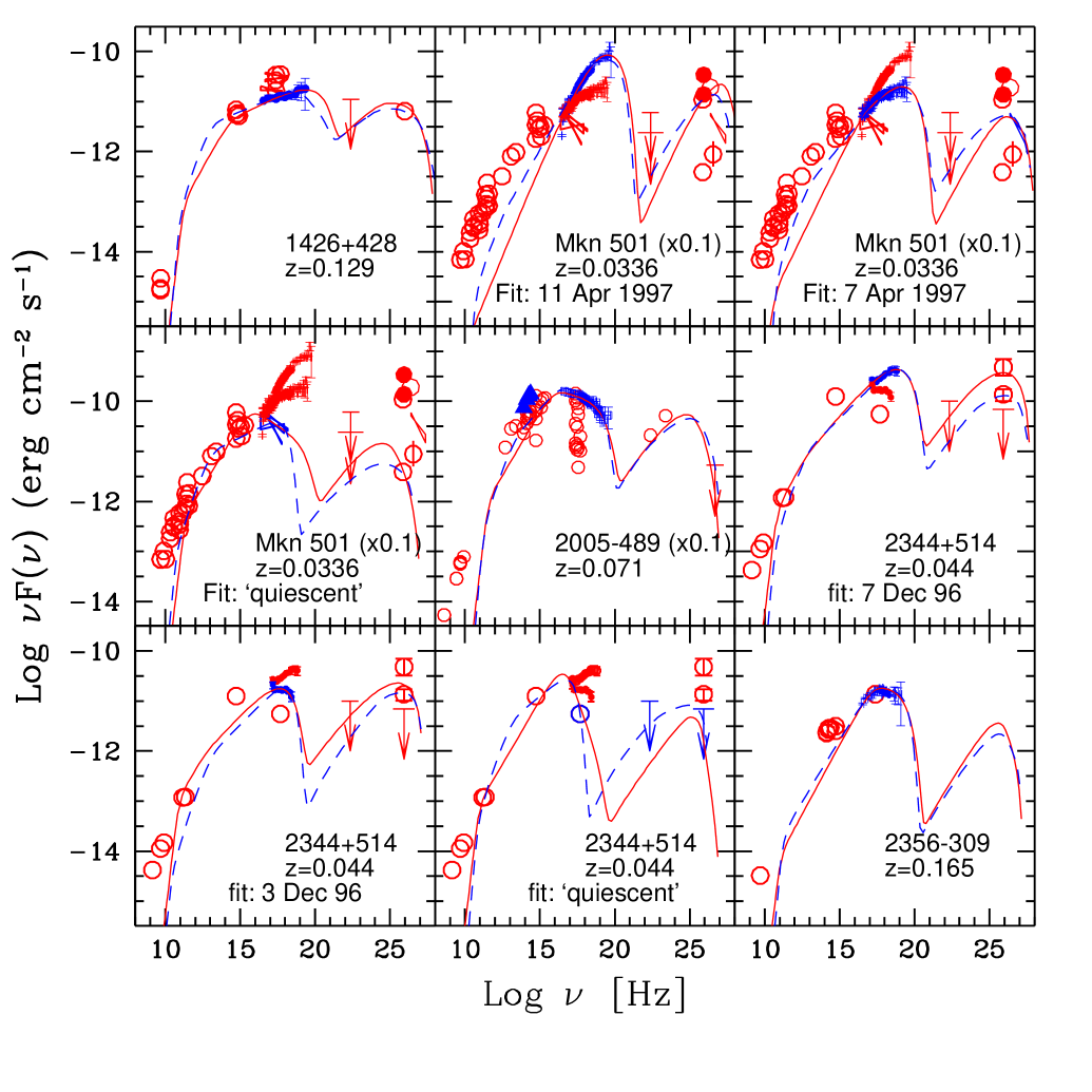
Figure 1: b): The SED of our extreme BL Lac objects. The solid and dashed lines correspond to the steady–state and finite injection time models, as discussed in Section 3 and 4, respectively.

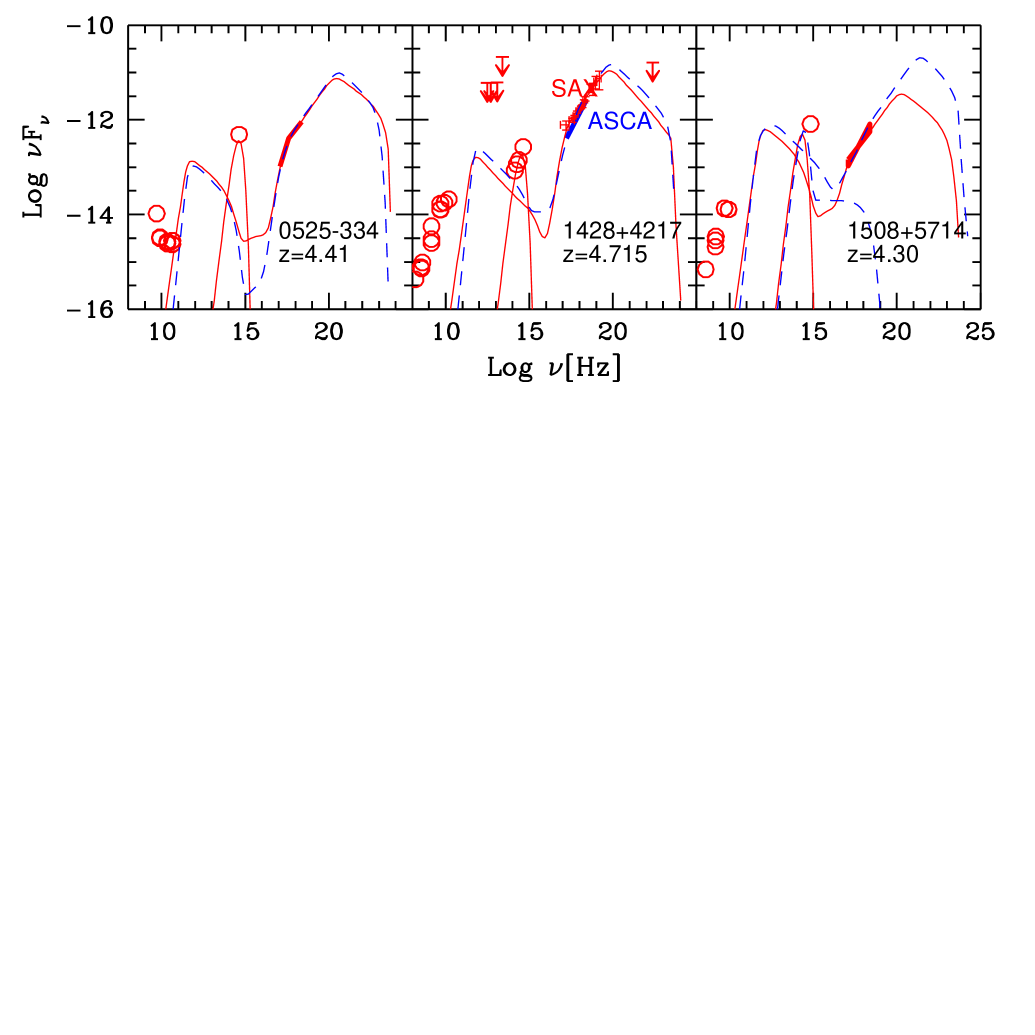
Figure 1: c): The SED of the 3 quasars at $z>4$ considered in this paper. The solid and dashed lines correspond to the steady–state and finite injection time models, as discussed in Section 3 and 4, respectively.

3 Steady–state synchrotron inverse Compton model

Source	$R$	$L^{\prime}_{\rm inj}$	$\gamma_{\rm min}$	$\gamma_{\rm max}$	$\gamma_{\rm peak}$	$s$	$B$	$\delta$	$L_{\rm ext}$	$R_{\rm ext}$	Notes
	cm	erg s-1					Gauss		erg s-1	cm
0033$+$595	5e15	1.8e41	9.0e4	1.2e6	9.0e4	2.0	0.73	15	—	—
0120$+$340	5e15	5.6e41	3.0e4	3.0e5	3.0e4	2.2	1.83	15	—	—
0548$-$322	5e15	4.3e40	8.0e4	8.0e5	8.0e4	2.1	0.51	15	—	—
1101$-$232	5e15	6.5e41	4.0e4	1.5e6	4.0e4	2.1	1.97	15	—	—
1101$+$384	5e15	3.3e41	1.0e5	1.0e6	1.0e5	2.5	0.34	15	—	—	1996 high state
1101$+$384	5e15	1.1e42	6.0e4	8.0e5	6.0e4	2.0	0.22	11	—	—	1994 flare (G98 fit)
1101$+$384	5e15	2.2e41	4.0e4	4.0e5	4.0e4	2.3	0.27	11	—	—	1994 pre–flare
1114$+$203	5e15	7.4e41	1.2e4	2.0e5	1.2e4	3.6	2.11	15	—	—
1218$+$304	5e15	6.5e41	1.0e4	4.0e5	1.0e4	3.0	3.11	15	—	—
1426$+$428	5e15	1.1e41	6.0e3	7.0e6	1.0e6	1.9	0.52	20	—	—
1652$+$398	5e15	1.7e41	1.0e6	9.0e6	2.5e6	1.4	0.10	20	—	—	11 Apr 1997
1652$+$398	5e15	4.6e40	7.0e4	5.0e6	1.4e6	1.4	0.17	20	—	—	07 Apr 1997
1652$+$398	5e15	3.7e41	1.0e4	8.0e5	1.0e4	2.8	1.11	10	—	—	quiescent, G98 fit
2005$-$489	5e15	6.5e41	1.0e4	7.0e5	1.0e4	2.2	2.20	15	—	—
2344$+$514	6e15	8.9e40	1.0e3	4.0e6	1.3e6	1.5	0.14	15	—	—	07 Dec 1996 high state SAX
2344$+$514	6e15	4.4e40	1.0e3	1.0e6	3.0e5	1.5	0.14	15	—	—	03 Dec 1996 low state SAX
2344$+$514	8e15	4.1e40	4.0e4	7.0e5	4.0e4	3.7	0.47	14	—	—	quiescent, G98 fit
2356$-$309	5e15	3.1e41	7.0e4	1.2e6	7.0e4	2.0	0.97	15	—	—
0525$-$334	2e16	1.4e44	45	2.0e3	45	2.5	5.13	15	5.0e45	8.0e17
1428$+$422	2e16	2.2e44	25	5.0e3	25	2.8	9.12	15	3.0e45	4.0e17
1508$+$571	2e16	7.4e43	50	2.0e3	50	2.5	11.8	15	6.6e45	1.2e18

Table 2: Parameters used to model the SED of the extreme BL Lacs (above the line) and powerful FSRQ (below the line) considered in this work, according to the steady–state synchrotron inverse Compton model as discussed in Section 3. $L_{\rm ext}$ and $R_{\rm ext}$ correspond to the luminosity and extension of the external photon source (assumed to originate in a Broad Line Region).

The SED of the considered sources have been modeled as in G98. We briefly remind the main assumptions of this model: in a spherical source of radius $R$, embedded in a tangled and homogeneous magnetic field $B$, a distribution of relativistic electrons is continuously injected at the rate $Q(\gamma)\propto\gamma^{-s}$ [cm^-3 s^-1] between $\gamma_{\rm min}$ and $\gamma_{\rm max}$, with a corresponding injected power $L_{\rm inj}^{\prime}$ as measured in the comoving frame. Note that $\gamma_{\rm min}$ is the minimum Lorentz factor of the injected electrons, and should not be confused with the minimum Lorentz factor of the emitting particle distribution, which is here assumed to extend down to $\gamma\sim 1$. The emitting particle distribution and corresponding spectrum are derived by solving the steady–state continuity equation, assuming synchrotron and inverse Compton radiative losses and possible pair production through photon–photon collisions. The seed photons for the inverse Compton process are both synchrotron and external photons, the latter ones assumed to be distributed as a (diluted) blackbody with peak frequency $\nu_{o}\sim 10^{16}$ Hz (as observed in the comoving frame). Externally produced radiation has been considered for the three high redshift quasars, while for all the extreme BL Lacs studied here the spectrum can be fitted with a pure synchrotron self–Compton (SSC) model, and we can therefore consistently neglect the presence of externally produced radiation.

For sources with $\gamma$–ray information we have enough data to completely constrain the SSC model. For the remaining objects we have to assume from the variability timescale $t_{var}$ the parameters $R$ and the bulk Lorentz factor $\delta$. We decided to adopt the same values of $\delta$ (=15) and $R$ ($=5\times 10^{15}$ cm) for all sources with no $\gamma$–ray data. Such values are in agreement with what we inferred for Mkn 501 and 1ES 1426+428 and with values reported by other authors in the literature (e.g. Mastichiadis & Kirk 1997; Tavecchio, Maraschi & Ghisellini 1998; Kataoka et al. 1999; Kino, Takahara & Kusunose, 2001). In the following we examine the dependence of the results on the assumption on $\delta$ . For the three high redshift quasars we have fixed the value of $\delta$ (=15, as for the other BL Lacs) and assumed a somewhat larger size of the emitting region ($R=2\times 10^{16}$ cm).

Note that the applied model is aimed at reproducing the spectrum originating in a limited part of the jet, thought to be responsible for most of the emission. This region is necessarily compact, since it must satisfy the constraints from the fast variability shown by blazars especially at high frequencies. Therefore the radio emission from such compact regions is strongly self–absorbed: the model cannot thus account for the observed radio flux.

In Table 2 we list all the input parameters used for the “fits” shown in Fig. 1a,b,c as solid lines, and we also report the value of the derived parameter $\gamma_{\rm peak}$.

In Fig. 2 we plot $\gamma_{\rm peak}$ as a function of the (comoving) energy density $U=U_{\rm r}+U_{B}$ (radiative plus magnetic) for these sources and those of G98. As in G98, the plotted radiation energy density $U_{\rm r}$ is not the total one, but only that part available for scattering in the Thomson regime for electrons of Lorentz factor $\gamma{\rm peak}$. Fig. 2 clearly shows that $\gamma_{\rm peak}$ and $U$ are still significantly correlated also for the more extreme objects, but, as expected, with a different functional dependence of $\gamma_{\rm peak}$ vs $U$: for values of $\gamma_{\rm peak}$ greater than $\sim 1000$ (corresponding to $U\lower 3.22916pt\hbox{$\sim$}\hbox to0.0pt{\hss\raise 1.1625pt\hbox{$<$}}1$ erg cm^-3), the new branch is approximately described by $\gamma_{\rm peak}\propto U^{-1}$. In Table 4 we give the statistical results of a linear correlation between $\log\gamma_{\rm peak}$ and $\log U$.

Let us consider the robustness of such finding with respect to our assumption on the Doppler factors. As mentioned above for Mkn 501 and 1ES 1426+428 the model parameters are completely determined by the spectral and variability information, while for the other sources we had to assume a value for the beaming factor $\delta$ (=15). Using for all of the new sources a lower (higher) value of $\delta$ would translate only into a shift of the $\gamma_{\rm peak}\propto U^{-1}$ branch towards higher (lower) $U$, not affecting its slope and thus its presence. Clearly, a spread in the values of $\delta$ would result in a scatter of the points around the correlation. Even in the fine tuned assumption of a systematic increase of $\delta$ – say between 10 and 20 – along the branch towards high $\gamma_{\rm peak}$, the slope would not change enough to recover the $\gamma_{\rm peak}\propto U^{-0.6}$ correlation. We conclude that the presence of the new steeper trend is robust.

On the other hand, we stress that the three powerful objects have been included in the sample in order to better test the presence of the flatter $\gamma_{\rm peak}\propto U^{-0.6}$ branch. Indeed as shown for example in the case of 1428+4217, the extension of the hard X-ray spectrum clearly constrains a minimum value of $\gamma_{\rm peak}$.

3.1 Interpretation

The existence of such good correlations between $\gamma_{\rm peak}$ and $U$ intriguingly suggests that these are the result of robust physical process(es). While, as already mentioned, the high $U$ branch corresponds to a constant (with respect to all other parameters) cooling rate at $\gamma_{\rm peak}$, the new steeper branch $\gamma_{\rm peak}\propto U^{-1}$ is equivalent to an approximately constant radiative cooling time $t_{\rm cool}(\gamma_{\rm peak})$. This appears to indicate that $\gamma_{\rm peak}$ might be determined by the cooling timescale approaching another relevant timescale of the system. Plausibly the most characteristic one would be the light crossing time associated to the dimension of the system. And indeed we find also quantitative indication from the parameters of the model that $t_{\rm cool}(\gamma_{\rm peak})\sim R/c$. Processes which can operate on such a timescale include adiabatic losses and/or particle escape (for expansion and escape velocities of order $\sim c$, see Kino, Takahara & Kusunose, 2001) or a particle injection (e.g. in a relativistic shock) lasting for $R/c$.

However the similarity of these two timescales also puts in evidence the inconsistency of the assumed model. More precisely if the typical cooling timescale for the particle radiating the bulk of the emission is of the order of the light crossing time, the assumption of steady state for deriving the particle distribution cannot be satisfied.

In such a situation therefore we have to consider a different scenario. In this respect two observational facts should be taken into account for the modeling of the emission. The variability characterizing blazars in general, and low power BL Lacs in particular, indicates that the deposition of energy is not continuous, but rather suggests a finite time of injection for each typical flare. Furthermore the symmetry of the raise and decay of flux in the light curves during flaring episodes, together with the absence of a plateau at constant flux, also indicates that the injection timescale should not exceed $R/c$ (Chiaberge & Ghisellini 1999). For these reasons we also explore here the situation where the injection lasts for a finite timescale, of order of the light crossing time.

A physical scenario where flares naturally occur and the injection timescale can be of order of the dynamical one is that of internal shocks (e.g. Piran 1999; Ghisellini 1999a; Spada et al. 2001), in which the dissipation takes place during the collision of two shells of fluid moving at different speeds. Let us then adopt such scenario.

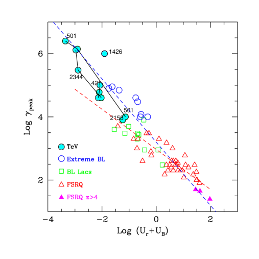
Figure 2: The Lorentz factor of the electrons emitting at the peaks of the SED, $\gamma_{\rm peak}$, as a function of the comoving energy density (radiative plus magnetic), according to the steady–state synchrotron self–Compton model, as discussed in Section 3. The points connected by a line correspond to the quiescent and flaring states of the same source, namely Mkn 501, Mkn 421 and 1ES 2344+514, as labeled. The dashed lines corresponds to the linear correlations found by G98 and the one found in this paper considering only BL Lac objects (see Table 4.

4 Finite injection time model

Source	$R$	$L^{\prime}_{\rm inj}$	$\gamma_{\rm min}$	$\gamma_{\rm max}$	$\gamma_{\rm peak}$	$s$	$B$	$\delta$	$L_{BLR}$	$R_{BLR}$	Notes
	cm	erg s-1					Gauss		erg s-1	cm
0033$+$595	9.0e15	1.0e41	1000	6.0e5	5.3e4	2.01	0.8	18.2	—	—
0120$+$340	1.0e16	4.4e41	700	2.5e5	7.0e4	2.2	0.6	18.6	—	—
0548$-$322	8.0e15	7.5e40	700	5.0e5	5.0e4	2.1	0.8	14.1	—	—
1101$-$232	7.0e15	5.3e41	2000	1.0e6	5.3e4	2.1	0.9	19.9	—	—
1101$+$384	1.5e16	3.3e42	1000	7.0e5	7.0e5	2.1	0.1	14.3	—	—	1996 flare
1101$+$384	1.7e16	1.4e42	800	5.5e5	5.5e5	2.1	0.08	14.3	—	—	flare
1101$+$384	1.7e16	1.5e41	800	3.8e5	3.8e5	2.4	0.08	14.3	—	—	Pre–Flare
1114$+$203	8.0e15	4.5e41	6000	2.0e5	6.0e3	3.6	1.5	18.8	—	—
1218$+$304	1.0e16	2.0e41	6000	3.0e5	1.4e4	2.9	1.5	19.3	—	—
1426$+$428	1.3e16	7.0e40	1000	6.0e6	7.2e5	2.7	0.18	25.1	—	—
1652$+$398	7.0e15	7.0e42	500	4.0e6	5.5e5	1.9	0.28	16.3	—	—	11 Apr 1997
1652$+$398	7.0e15	6.0e41	200	4.0e6	4.5e5	2.26	0.3	16.3	—	—	07 Apr 1997
1652$+$398	1.8e16	2.5e40	1000	3.0e5	3.0e5	2.7	0.24	16.3	—	—	quiescent
2005$-$489	1.0e16	8.0e41	600	5.0e5	1.3e4	2.3	1.5	15.5	—	—
2344$+$514	1.2e16	6.0e41	2000	2.4e6	1.6e6	2.4	0.11	14.2	—	—	7 Dec 1996 high state
2344$+$514	1.2e16	1.2e41	2000	8.0e5	8.0e5	2.4	0.09	14.2	—	—	3 Dec 1996 low state
2344$+$514	1.e16	5.0e40	1000	1.0e5	1.0e5	2.5	0.4	14.2	—	—	quiescent
2356$-$309	7.0e15	2.0e41	100	7.0e5	6.0e4	2.01	0.9	18.8	—	—
0525$-$334	2.0e16	6.0e43	60	1.0e3	60.0	2.7	10	19.0	1.1e46	2.0e17
1428$+$422	2.0e16	5.0e44	33	2.0e3	33.0	2.7	11	12.6	8.0e45	2.5e17
1508$+$571	3.0e16	6.0e44	200	8.0e3	200	2.7	14	12.7	1.2e45	4.0e17

Table 3: Parameters used to model the SED of the extreme BL Lacs and powerful FSRQ (above and below the horizontal line, respectively) considered in this paper, according to the finite injection time synchrotron inverse Compton model as discussed in Section 4. $L_{BLR}$ and $R_{BLR}$ correspond to the equivalent luminosity and extension of the external photon energy density (assumed to originate in a Broad Line Region).

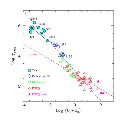
Figure 3: The Lorentz factor of the electrons emitting at the peaks of the SED, $\gamma_{\rm peak}$, as a function of the comoving energy density (radiative plus magnetic), according to the finite injection time synchrotron inverse Compton model as discussed in Section 4. The points connected by a line correspond to the quiescent and flaring state of the same source, namely Mkn 501, Mkn 421, 1ES 2344+514, as labeled. The dashed lines correspond to $\gamma_{\rm peak}\propto U^{-1/2}$ and $\propto U^{-1}$ (they are not best fits).

Model	$m$	$q$	$N$	$r$	$P$
Steady st. (BL)	$-$0.958$\pm$0.11	3.10$\pm$0.18	30	$-$0.86	7.3e-8
Fin. inj. (BL)	$-$0.975$\pm$0.06	2.94$\pm$0.12	30	$-$0.95	7.5e-8
Steady st. (FSRQ)	$-$0.565$\pm$0.06	2.88$\pm$0.06	44	$-$0.84	4.4e-8
Fin. inj. (FSRQ)	$-$0.544$\pm$0.06	2.79$\pm$0.05	44	$-$0.82	1.5e-8

Table 4: Results of linear correlations between $\log\gamma_{\rm peak}$ and the total energy density $\log U$ (magnetic plus radiative) in the comoving frame. We have fitted separately all BL Lac objects, including the extreme sources studied in this paper, and all FSRQ, including the three high redshift quasars studied here. The correlation is in the form $\log\gamma_{\rm peak}=m\log U+q$. $P$ is the probability of a random distribution and $r$ the correlation coefficient.

As in the steady state model just considered, the magnetic field is assumed to be homogeneous and tangled throughout the region. Note however that in the internal shock scenario the geometry of the emitting volume is a cylinder with thickness $\Delta R^{\prime}\sim R/\Gamma$ (in the comoving frame) and radius $R$ corresponding to the cross section of the jet. In the following we thus adopt such geometry and again assume $\Gamma\sim\delta$.

In the hypothesis of a finite injection time $t_{\rm inj}$, which we assume lasts for $t_{\rm inj}=\Delta R^{\prime}/c$, clearly the continuity equation governing the particle distribution has no steady state solution (see also Sikora et al. 2001). However since we are studying variable (flaring) sources, a reasonably good representation of the observed spectrum can be obtained by considering the particle distribution at the time $t_{\rm inj}$, i.e. at the end of the injection, where in fact the emitted luminosity is maximized.

Beside the geometrical difference, clearly the main (and possibly crucial as far as the interpretation is concerned) difference between the steady–state and the finite injection hypothesis is related to the shape of the emitting particle distribution. In fact in the latter scenario $\gamma_{\rm peak}$ does not have to be associated with the minimum energy of the injected particles (as was the case so far in our modeling). If the injection lasts for a finite timescale, only the higher energy particles have the time to cool and therefore the particle distribution can be described as a broken power–law with a steep part above $\gamma_{\rm peak}$ and the original injection slope below. In other words $\gamma_{\rm peak}$ results to be defined by the condition $t_{\rm cool}(\gamma_{\rm peak})=t_{\rm inj}$, while the minimum energy $\gamma_{\rm min}$ can be much smaller than $\gamma_{\rm peak}$.

More precisely, let us define $\gamma_{\rm c}$ as the energy of those electrons that can cool in the injection time $t_{\rm inj}$, i.e. $t_{\rm cool}(\gamma_{\rm c})=t_{\rm inj}$. At energies greater than $\gamma_{\rm c}$, particles radiatively cool, and the distribution reaches a steady state in a time smaller than $t_{\rm inj}$. The particle distribution $N(\gamma)$ will be then described according to the following prescriptions:

• If $\gamma_{\rm c}>\gamma_{\rm max}$, then no particles cool in the injection time and we assume that $N(\gamma)\propto\gamma^{-s}$ above $\gamma_{\rm min}$, and $N(\gamma)\propto\gamma^{-1}$ below.

• If $\gamma_{\rm min}<\gamma_{\rm c}<\gamma_{\rm max}$, we assume that $N(\gamma)\propto\gamma^{-(s+1)}$ above $\gamma_{\rm c}$, $N(\gamma)\propto\gamma^{-s}$ between $\gamma_{\rm min}$ and $\gamma_{\rm c}$ and $N(\gamma)\propto\gamma^{-1}$ below $\gamma_{\rm min}$.

• If $\gamma_{\rm c}<\gamma_{\rm min}$ then $N(\gamma)\propto\gamma^{-(s+1)}$ above $\gamma_{\rm min}$; $N(\gamma)\propto\gamma^{-2}$ between $\gamma_{\rm c}$ and $\gamma_{\rm min}$ and $N(\gamma)\propto\gamma^{-1}$ below $\gamma_{\rm c}$.

• If electron of all energies radiatively cool in the time $t_{\rm inj}$, then $N(\gamma)\propto\gamma^{-(s+1)}$ above $\gamma_{\rm min}$ and $N(\gamma)\propto\gamma^{-2}$ below.

We note here that even if the shape of $N(\gamma)$ is not formally derived by solving the continuity equation, it does correspond to the shape expected from injecting a broken power–law with a break at $\gamma_{\rm min}$, and slopes $\propto\gamma^{-1}$ and $\propto\gamma^{-s}$ below and above.

With these prescriptions we then modeled all SEDs. In Table 3 we list the input parameters used (plus the derived value of $\gamma_{\rm peak}$) for the spectra shown in Fig. 1a,b,c as dashed lines. It is apparent that the accuracy of the representation of the SED is comparable with that obtained in the stationary assumption, and does not allow to discriminate between the two models.

In Fig. 3 we show $\gamma_{\rm peak}$ as a function of the comoving energy density $U$ according to the application of this model to $all$ sources, the sources analyzed in this paper plus those considered in G98 for consistency. As expected, for powerful blazars (large $U$, small $\gamma_{\rm peak}$) we do not find significant differences with respect to the results of the previous model (compare the branches at high $U$ of Fig. 2 and Fig. 3), since for these sources $\gamma_{\rm c}\ll\gamma_{\rm min}$, and therefore $\gamma_{\rm peak}\sim\gamma_{\rm min}$ in both scenarios. However, for small values of $U$, $\gamma_{\rm peak}$ coincides with $\gamma_{\rm c}>\gamma_{\rm min}$ and this automatically ensures that $\gamma_{\rm peak}\propto U^{-1}$, except when $\gamma_{\rm c}$ results to be so large to exceed $\gamma_{\rm max}$ (in this case, of course, $\gamma_{\rm peak}=\gamma_{\rm max}$). In the finite injection model, in fact, the relation $\gamma_{\rm c}\propto U^{-1}$ is built–in, and translates into a $\gamma_{\rm peak}\propto U^{-1}$ when $\gamma_{\rm c}>\gamma_{\rm min}$. What we have verified is that this model fits the SEDs of all blazars, including the powerful ones. For the latter (i.e. large $U$ and small $\gamma_{\rm peak}$) we find the same correlation as found using the steady state model. We conclude that also this more consistent scenario confirms the existence of the two branches. These connect, as before, for values of $U\sim$ a few erg cm^-3 and $\gamma_{\rm peak}\sim 300$. This is a consequence of $\gamma_{\rm c}$ becoming smaller than $\gamma_{\rm min}$ caused by the increased radiative cooling in powerful blazars.

5 Summary and conclusions

By studying blazars of very high and very small observed power we have confirmed that different flavors of blazars form a spectral and power sequence, where the peak frequency position and the relative intensity of the low and high energy spectral components decrease with increasing source power.

This phenomenological behavior is plausibly the manifestation of a physical trend. By (necessarily) adopting an emission model for the production of the radiation, it is then possible to infer the physical parameters and look for the process(es) responsible for it.

In particular we considered the emission via synchrotron and inverse Compton scattering by a homogeneous region containing a tangled magnetic field and relativistic electrons. Already in a previous study (G98) this resulted in the finding of a clear relationship between the energy of the particles emitting at the peaks of the spectrum $\gamma_{\rm peak}m_{e}c^{2}$ and the total energy density. Here we extended the range of parameters by including sources with more extreme values of $\gamma_{\rm peak}$. The physical conditions found for low power BL Lacs imply a radiative cooling timescale long compared with the source light crossing time, and led us to consider the effects of a finite time $t_{\rm inj}$ for the injection of the relativistic particles.

The modeling of the blazar SED including a finite injection timescale (e.g. plausibly resembling what expected in the internal shock scenario) confirms the existence of a new branch of the correlation at high $\gamma_{\rm peak}$, with $\gamma_{\rm peak}\propto U^{-1}$. As the injection of particles above an energy $\gamma_{\rm min}m_{\rm e}c^{2}$ lasts for $t_{\rm inj}$ we obtain two behaviors: in the fast cooling regime $\gamma_{\rm peak}\sim\gamma_{\rm min}$ and we re–obtain the result of G98, while in the slow cooling regime $\gamma_{\rm peak}$ corresponds to particles whose cooling time equals the injection time. In this case $\gamma_{\rm peak}$ is always greater than $\gamma_{\rm min}$ and we obtain $\gamma_{\rm peak}\propto U^{-1}$.

While these results and their interpretation do not reveal the acceleration mechanism itself, they are suggestive of the fact that two processes maybe at work: a phase of (pre–)heating determining $\gamma_{\rm min}$, and a phase of rapid acceleration leading to a non–thermal distribution. If so the typical energy produced by the pre–heating (in the range $\gamma_{\rm min}\sim$ 30–10³) would correspond to the balancing between heating and cooling rates, which would give the $\gamma_{\rm min}\propto U^{-0.5}$ dependence. The second phase, reminiscent of acceleration at shocks, would have to be a fast (“instantaneous”) acceleration of particles according to a power–law distribution. The energetic particles would then cool (as in post–shock plasma) and after a time $t_{\rm inj}$ the particles above $\gamma_{\rm c}$ would have cooled according to $\gamma_{\rm c}\propto U^{-1}$. Although this interpretation might sound rather speculative, we stress that the occurrence of these two phases is indeed needed in the context of particle acceleration by shocks.

We also note that, in the framework of the adopted finite time injection model, we cannot reproduce the SED of blazars by imposing that a single mechanism is at work, namely by fixing $\gamma_{\rm min}$ to a constant value for all blazars and letting only $\gamma_{\rm c}$ to assume the value appropriate for the particular cooling conditions. In this case, in fact, we would be forced to assume $\gamma_{\rm min}\sim$a few for all blazars (to properly fit the powerful ones) with a particle distribution $N(\gamma)\propto\gamma^{-s}$ between $\gamma_{\rm min}$ and $\gamma_{\rm c}$. As a result, we would overestimate the flux of our extreme BL Lacs at frequencies below the synchrotron peak, which instead require $\gamma_{\rm min}\lower 3.22916pt\hbox{$\sim$}\hbox to0.0pt{\hss\raise 1.1625pt\hbox{$>$}}10^{3}$.

An important point to be considered in interpreting the above findings is that they refer to an average state of the source within the proposed blazar sequence. However, individual flares have been observed to behave also differently: a specific source can vary by a significant factor in the direction opposite to the sequence trend, i.e. both $\gamma_{\rm peak}$ and the observed luminosity can increase at the same time (e.g. Mkn 501 during its 1997 active state). The correlation between $\gamma_{\rm peak}$ and the comoving energy density still holds even in these cases (see the “tracks” shown in Fig. 2 and Fig. 3 for the TeV BL Lacs modeled in different states), but it is important to notice that in the case of the flaring state of Mkn 501 the particle distribution is found to be quite flat (i.e. $N(\gamma)\propto\gamma^{-(s+1)}$ with $s<2$), at variance with the typical values generally found (i.e. $s>2$, see Table 3). This implies values of $\gamma_{\rm peak}$ close to $\gamma_{\rm max}$ irrespective of the amount of radiative cooling. Physically, this suggests that when the source undergoes major flares, the shock acceleration mechanism becomes energetically dominant with respect to the pre–heating process, leading to flat particle distributions and thus to flat spectra in the entire synchrotron frequency range.

Let us conclude by asking whether there is any physical limit to the value of $\gamma_{\rm peak}$. BL Lac objects even more extreme than Mkn 501 could exist, with their synchrotron peak frequency reaching the MeV band. The found trends suggest that the most extreme values of $\gamma_{\rm peak}$ are possible only in sources intrinsically weak in the radio and optical band which could have thus escaped so far from being recognized as BL Lac objects in existing samples (see e.g. Ghisellini 1999b). As in the radio and optical band the SED would presumably be dominated by the emission from the host galaxy, these putative sources might resemble low power radio galaxies (such as those of the B2 sample). Their BL Lac–ness should appear evident in the TeV band and at hard X–ray energies, although care should be taken not to confuse their emission with the similarly hard X–ray spectra produced by e.g. low radiative efficiency accretion model (where the radiation is via free free or thermal Comptonization).

- (1) Bersanelli et al. 1992, AJ, 104, 28 (Be92)
- (2) Bohringer H., Voges W., Huchra J.P. et al., 2000, ApJS, 129, 435
- (3) Brinkmann W., Siebert J., Feigelson E.D. et al., 1997, A&AS, 323, 739 (Br97)
- (4) Brinkmann W. & Siebert, 1994, A&A, 285, 812 (BS94)
- (5) Catanese M., & Weekes T.C., 1999, PASP, 111, 1193
- (6) Chiaberge M. & Ghisellini G., 1999, MNRAS, 306, 551
- (7) Costamante L., Ghisellini G., Giommi P. et al., 2001, A&A, 371, 512 (Co01)
- (8) Fabian A.C., Celotti A., Iwasawa K., McMahon R.G., Carilli C.L., Brandt W. N., Ghisellini G. & Hook I.M., 2001a, 323, 373 (Fa01a)
- (9) Fabian A.C., Celotti A., Iwasawa K. & Ghisellini G., 2001b, MNRAS, 324, 628 (Fa01b)
- (10) Falomo R., Scarpa R. & Bersanelli M., 1994, ApJS, 93, 125 (Fa94)
- (11) Falomo R. & Kotilainen J., 1999, A&A, 352, 85
- (12) Fichtel C.E., Bertsch D.L., Chiang J., et al. 1994, ApJS, 94, 551 (Fi94)
- (13) Fossati G., Maraschi L. Celotti A., Comastri A. & Ghisellini G., 1998, MNRAS, 299, 433 (F98)
- (14) Ghisellini G., Celotti A., Fossati G., Maraschi L. & Comastri A., 1998, MNRAS, 301, 451 (G98)
- (15) Ghisellini G., 1999a, 4th ASCA Symp., Astronomische Nachrichten. Editors: H. Inoue, T.Ohashi & T.Takahashi, 320, p. 232
- (16) Ghisellini G., 1999b, in: TeV Astrophysics of Extragalactic Objects, Astroparticle Physics, Eds. M. Catanese & T. Weeks, Vol. 11, Issue 1–2, p. 11–18
- (17) Giommi P., Ansari S.G. & Micol A., 1995, A&AS, 109, 267 (GAM95)
- (18) Giommi P. & Padovani P., 1994, MNRAS, 268, L51
- (19) Giommi P., Padovani P. & Perlman E., 2000, MNRAS, 317, 743 (GI00)
- (20) Horan D. VERITAS collaboration, 2000, HEAD meeting, No 23, 05.03 (Ho00)
- (21) Kataoka J., Mattox J.R., Quinn J., et al., 1999, ApJ, 514, 138
- (22) Kino M., Takahara F. & Kusunose M., 2001, ApJ, in press (astro–ph/0107436)
- (23) Lamer G., Brunner H., & Staubert R., 1996, A&A, 311, 384 (La96)
- (24) Macomb J., Akerlof C.W., Aller H.D. et al. 1995, ApJ, 449, L99 (Ma95)
- (25) Macomb J., Akerlof C.W., Aller H.D. et al. 1996, ApJ, 459, L111 (erratum) (Ma96)
- (26) Mastichiadis A. & Kirk J.G., 1997, A&A, 320, 19
- (27) Moran E.C. & Helfand D.J., 1997, ApJ, 484, L95 (MH97)
- (28) Padovani P. & Giommi P., 1995, ApJ, 444, 567
- (29) Padovani P. & Urry C.M., 2001, Blazar Demographics and Physics, ASP Conf Series, 227
- (30) Perlman E.S, Stocke J.T., Schachter J.F., et al., 1996, ApJS, 104, 251 (Pe96)
- (31) Pian E. & Treves A., 1993, ApJ, 416, 130 (Pi93)
- (32) Pian E., Vacanti G., Tagliaferri G. et al., 1998, ApJ, 491, L17
- (33) Piran T., 1999, Phys. Rep., 314, 575
- (34) Sambruna R.M., Barr P., Maraschi L., Tagliaferri G. & Treves A., 1993, ApJ, 408, 452 (Sa93)
- (35) Sambruna R.M., Barr P., Giommi P., Maraschi L., Tagliaferri G. & Treves A., 1994, ApJS, 95, 37 (Sa94)
- (36) Sambruna R.M., George I.M., Madejski G., Urry C.M., Turner T.J., Weaver K.A., Maraschi L. & Treves, A., 1997, ApJ, 483, 774 (Sa97)
- (37) Schubnell M., 1997, Proceedings of the Fourth Compton Symposium, Eds C.D. Dermer, M.S. Strickman & J.D. Kurfess, AIP Conference Proceedings 410, p. 1386 (astro–ph/9707047)
- (38) Sikora M., Blazejowski M., Begelman M.C. & Moderski R., 2001, ApJ 544, 1.
- (39) Sikora M. & Madejski G., 2001, in: International Symposium on High Energy Gamma-Ray Astronomy, Heidelberg, Eds. F. Aharonian and H. Voelk, 2001, AIP, in press (astro–ph/0101382)
- (40) Stevens, J. & Gear 1999, MNRAS, 307, 403 (SG99)
- (41) Stocke J.T., Morris S.L., Gioia I.M., Maccacaro T., Schild R., Wolter A., Fleming T.A., Henry J.P. 1991, ApJS, 76, 813
- (42) Tagliaferri G., Ghisellini G., Giommi P. et al., 2001, A&A, 368, 38 (Ta01)
- (43) Tashiro M., Makishima K., Ohashi T., Inda–Koide M., Yamashita A., Mihara T., Kohmura Y., 1995, PASJ, 47, 131 (Ta95)
- (44) Tavecchio F., Maraschi L. & Ghisellini G., 1998, ApJ, 509, 608
- (45) Wolter A., Tavecchio F., Caccianiga A., Ghisellini G. & Tagliaferri G., 2000, A&, 357, 429 (Wo00)
- (46) Worral D.M. & Wilkes B.J., 1990, ApJ, 360, 396 (WW90)