Predictions for Fourier-resolved X-ray spectroscopy from the model of magnetic flare avalanches above an accretion disc with hot ionized skin

Abstract

The magnetic flare avalanches model of Poutanen & Fabian for X–ray variability of accreting black holes is combined with computations of vertical structure of illuminated accretion discs in hydrostatic equilibrium. The latter predict the existence of a hot ionized skin, due to the thermal instability of X–ray illuminated plasma. The presence of such ionized skin, with properties dependent on disc radius, introduces a dependence of the emitted X–ray spectrum on the position on the disc. If the position is related to the time scale of the flares, the X–ray energy spectra (both the primary continuum and the reprocessed component) gain an additional dependence on Fourier frequency, beside that resulting from spectral evolution during a flare. We compute the Fourier frequency resolved spectra in this model and demonstrate that the presence of the hot skin introduces trends opposite to those observed in black hole binaries. Furthermore, the flare profile is strongly constrained, if the Fourier frequency dependence due to spectral evolution is to agree with observations.

1 Introduction

X–ray emission from accreting compact objects carries information about geometry and physical conditions in the immediate vicinity of central objects. Unfortunately, the information is “encrypted” into a series of numbers, each number (event) corresponding to a detection of a photon from the source. Two main characteristics of each event are the photon energy and arrival time (we neglect here polarization of radiation). One way of analyzing the data stream is then to project the events onto the energy axis, thus suppressing the timing information. Thus obtained energy spectra give a first, rough insight into physical mechanism of emission of radiation. For example, observations of cutoffs at $\sim 100$ keV in low/hard state of accreting black holes demonstrate that the Comptonizing electrons have a thermal rather than non-thermal distribution. From modelling the spectra a mean plasma temperature and scattering optical depth can be inferred. However, any possible distributions of plasma temperature and density cannot be recovered from time-averaged spectra (e.g. Kazanas, Hua & Titarchuk 1997; Coppi 1999).

In an analogous way, projecting the data onto the time axis produces a light curve, which can be analyzed either in the time or Fourier domain. The results, too, enable determination of certain average properties. For example from power spectral density (PSD), the root mean square variability or constraints on distribution of shots’ time scales in the shot noise model can be found (Lehto 1989; Lochner, Swank & Szymkowiak 1991).

Further progress can be made by including at least limited information from along the other parameter axis. For example, cross-correlation analysis (both in time and Fourier domain) reveal that higher energy X–rays lag the lower energy ones (Miyamoto & Kitamoto 1989), which one can attempt to interpret as e.g. spectral evolution during a shot (flare). Then the energy dependent auto-correlation functions give average shot profiles as a function of energy (see review in Poutanen 2001 and references therein).

Similarly, studying a sequence of energy spectra, each one averaged over a certain short time interval, enables determination of not only the mean spectral properties, but also “higher orders” statistics properties. The most important result that has emerged recently is that spectral properties of a given source vary with time, but correlations between parameters exist. The power law slope, $\Gamma$, is correlated with the amplitude of reflection $R$ and the width of the Fe K_α line (Zdziarski, Lubiński & Smith 1999; Gilfanov, Churazov & Revnivtsev 1999; Revnivtsev, Gilfanov & Churazov 2001; Życki, Done & Smith 1998). Interestingly, the same correlations seem to exist between sources in a sample (Zdziarski et al. 1999; Lubiński & Zdziarski 2001).

A number of geometrical/physical scenarios can be built based on the $R$–$\Gamma$ correlation alone. The crucial element of all models is the feedback between the hot, X–ray emitting plasma and the cooler, optically thick plasma: most of the soft photons crossing the hot plasma have to come from thermalization/reprocessing of the illuminating hard X–rays (Poutanen 1998 and references therein). Given this condition alone, models can be constructed belonging to two main classes, (1) with the standard accretion disc disrupted at a certain radius, and (2) with the standard accretion disc extending to the last stable orbit:

• standard accretion disc disrupted at a given radius, and filled with hot, optically thin, X–ray producing flow (Esin, McClintock & Narayan 1997; Poutanen, Krolik & Ryde 1997; Różańska & Czerny 2000), with the amount of overlap between the two phases controlling the correlations,

• hot, optically thin, quasi-spherical flow with cold cloudlets inside (Rees 1987; Kuncic, Celotti & Rees 1997), with the cloudlets filling factor controlling the correlations,

• spherical accretion of cold clouds onto a central X–ray source (Collin-Souffrin et al. 1996; Malzac 2001), with the covering factor of the clouds as the control parameter,

• mildly relativistic outflow of the X–ray emitting plasma, above a standard accretion disc, with the outflow velocity controlling the correlations (Beloborodov 1999a,b; Janiuk, Czerny & Życki 2000; Malzac, Beloborodov, Poutanen 2001),

• hot, ionized skin on top of the accreting disc, due to thermal instability of the X–ray illuminated plasma, with the skin thickness as the control parameter (Różańska & Czerny 1996; Nayakshin, Kazanas & Kallman 2000; Życki & Różańska 2001).

Also, models for time variability predicting correct PSD, time lags and coherence function can be constructed for the two main geometries (Poutanen & Fabian 1999, hereafter PF99; Böttcher & Liang 1999; review in Poutanen 2001). Therefore, based solely on the limited spectral/temporal data distinguishing between these scenarios appears very difficult, if at all possible (see e.g. discussion and application to Cyg X-1 in Di Salvo et al. 2001). Employing more sophisticated tools, involving both spectral and temporal properties is clearly required.

The Fourier frequency resolved ($f$-resolved hereafter) energy spectra seem to be a potentially powerful tool to apply to the problem of distinguishing the models. The $f$-resolved spectra are energy spectra in the limited range of Fourier frequency and so, roughly speaking, represent spectra at different time scales of variability (Revnivtsev, Gilfanov & Churazov 1999; Gilfanov, Churazov & Revnivtsev 2000a,b). The $f$-resolved spectra found from data of X-ray binaries show a number of features and correlations. Most importantly, the $R$-$\Gamma$ correlation is fulfilled by the $f$-resolved spectra in the sense that the higher the Fourier frequency, the harder the spectrum, and the smaller the amplitude of reflection (Revnivtsev et al. 1999). This result indicates that the same mechanism which is responsible for the correlation on long timescales ($\sim 10^{3}$ sec $\approx 10^{5}$–$10^{6}t_{\rm dyn}$, $t_{\rm dyn}=\Omega_{\rm K}^{-1}$ being the dynamical timescale), acts also on much shorter time scales, at least down do $\sim 0.01$ sec, the time bin of the Revnivtsev et al. analysis. This fact provides the motivation for our attempt to connect the spectral and timing models and predict their combined results. Therefore in this paper we consider a simple combination of the model of PF99, with the structure of illuminated accretion discs in hydrostatic equilibrium. The former is the most complete X–ray emission model so far, since it addresses both the spectral and timing properties of Comptonization emission. The latter naturally predicts the appearance of a hot, ionized skin on top of the disc (Różańska & Czerny 1996; Nayakshin et al. 2000), as a result of the thermal instability of the X-ray irradiated plasma (Field 1965; Krolik, McKee & Tarter 1981). The ionized skin reduces the effectiveness of reprocessing and thermalization of the hard X–rays. The flux of soft photons is reduced, which may lead to a harder continuum spectrum. If the ionized skin is thickest close to the black hole (Nayakshin 2000; Życki & Różańska 2001), then the hardest spectra, with lowest reflection amplitude are expected to originate there. If the short time scale (high Fourier frequency, $f$) flares originate close to the black hole, then one may expect the high-$f$ spectra to be harder, and show less reflection compared to low-$f$ spectra, precisely as observed from accreting black hole binaries.

The plan of the paper is as follows: in Section 2 we define the model, in Section 3 we perform some test computations to gain deeper insight into the properties of frequency-resolved spectra, Section 4 contains results of full model calculations and their comparison with data; the results are discussed in Section 5.

2 The Model

2.1 Time variability

We envision that the X–rays are produced in flares occurring above an accretion disc. The variability part of our model is therefore identical to that of PF99 (see also Stern & Svensson 1996), so only a brief description is given here for completeness. There is a number of spontaneous flares, $\lambda$ per second, each of which can give rise to an avalanche of stimulated flares. The number of stimulated flares is drawn from a Poissonian distribution with the mean $\mu$. Each stimulated flare is delayed from the stimulating flare by an interval $\Delta t$, drawn from a Poissonian distribution of mean $\alpha\tau_{1}$, where $\tau_{1}$ is the time scale of the stimulating flare while $\alpha$ is a parameter. The time scales of all flares are drawn according to a power law probability distribution $\propto\tau^{-p}$ between $\tau_{\rm min}$ and $\tau_{\rm max}$.

As in PF99 all flares have the same profile, which describes the heating of electrons as a function of time, $l_{\rm h}(t)$. Here, $l_{\rm h}$ is the compactness parameter, $l\equiv L\sigma_{\rm T}/(R_{\rm flare}m_{\rm e}c^{3})$, where $L$ is the luminosity and $R_{\rm flare}$ is the radius of a flare. The flare profile turns out to be decisive for the obtained dependence of energy spectra on Fourier frequency, therefore we will employ two of prescriptions:

• the function used by PF99,

  $$l_{\rm h,1}(t)\propto(t/\tau)^{2}\exp(-t/\tau),$$ (1)

• a double exponential function defined as

  $$l_{\rm h,2}(t)\propto\left\{\begin{array}[]{lc}\exp(t/\tau_{\rm r}),&\mbox{for $t<0$}\\ \exp(-t/\tau_{\rm d}),&\mbox{for $t>0$},\end{array}\right.$$ (2)

  where $\tau_{\rm r}$ and $\tau_{\rm d}$ represent the rise and decline time scales and $\tau_{\rm r}\gg\tau_{\rm d}$ (Maccarone, Coppi & Poutanen 2000).

The functions are normalized to give an assumed value of peak compactness, $l_{\rm h,max}$, for which we adopt $l_{\rm h,max}=10$. The flare decline time scale is assumed $\tau_{\rm d}=0.1\tau_{\rm r}$.

The flux of soft photons through the flare is given as $l_{\rm s}(t)=l_{\rm s,0}+D(t)l_{\rm h}(t)$ (PF99), where the second term describes the feedback due to reprocessing of the hard X–rays. Here, our first extension of the PF99 model is introduced: the feedback expression contains a factor describing the effectiveness of thermalization due to the ionized skin,

$$D(t)=S(t)\,{D_{0}\over 1+3\left[H(t)\right]^{2}}.$$ (3)

Here $S(t)=S[\tau_{\rm hot}(t)]$ is the fraction of the illuminating hard X–rays that get through the ionized skin to the cold disc, as a function of $\tau_{\rm hot}$ (equation 11), $D_{0}$ is a parameter, while $H(t)$ is the height of the flare above the disc.

2.2 Radial dependencies

The crucial extension of the PF99 model which needs to be made here is to relate the time scale of a flare to its radial location on the accretion disc. We will consider two cases:

1. There is a unique correspondence between the time scale of an individual flare (both spontaneous and stimulated) and its location on the disc. Since we do not assume any correlation between time scales of a stimulating and stimulated flare, this means that spatial locations of flares within an avalanche are not correlated.

2. The unique correspondence between $\tau$ and $r$ holds for spontaneous flares, while all flares stimulated by a given spontaneous flare occur at the location of the latter (Merloni & Fabian 2001).

The essential assumption here is that there is at least partial correspondence between flare’s time scale and its radial position. To quantify the discussion we assume that the flare time scale has the same radial dependence as the inverse of the Keplerian frequency, $\tau\propto r^{3/2}$. Moreover, the shortest flare time scale is assumed to correspond to the marginally stable orbit at $6r_{\rm g}=6GM/c^{2}$. This gives

$$r=6r_{\rm g}\left({\tau\over\tau_{\rm min}}\right)^{2/3}.$$ (4)

One consequence of such assumption is the existence of the maximum radius of the flares-covered disc, $r_{\rm max}=6r_{\rm g}\left(\tau_{\rm max}/\tau_{\rm min}\right)^{2/3}\approx 170r_{\rm g}$.

Some other parameters of the model need to be considered as functions of radius, too. The compactness

$$l_{\rm s,0}\equiv\pi R_{\rm flare}F_{\rm disc}{\sigma_{\rm T}\over m_{\rm e}c^{3}}$$ (5)

(see equation 1 in PF99) is a function of radius, since both the internal disc emission, $F_{\rm disc}$, and the flare’s radius, $R_{\rm flare}$ may in general be functions of radius. For the internal disc emission we adopt the standard, Newtonian formula (Shakura & Sunyaev 1973)

$$F_{\rm disc}(r)=\xi F_{\rm tot}(r)=\xi\,{3\over 8\pi}{GM{\dot{M}}\over r^{3}}\left(1-\sqrt{6\,r_{\rm g}\over r}\right),$$ (6)

where $\xi$ is the fraction of total energy dissipated inside the disc ($1-\xi$ dissipated in the active corona). We will assume that the radius of a flare, $R_{\rm flare}$, is constant with the radial position. The value of $R_{\rm flare}$ will be derived from global energy budget for the hot plasma: the total, time-integrated luminosity of all flares equals energy dissipation in the hot phase,

$${m_{\rm e}c^{3}\over\sigma_{\rm T}}\sum_{i=1}^{N}\int_{0}^{T}\,l_{{\rm h},i}(t)R_{{\rm flare},i}\,dt=(1-\xi)L_{\rm tot}T,$$ (7)

where the sum is over all flares, $L_{\rm tot}=\int_{6r_{\rm g}}^{\infty}2\pi rF_{\rm tot}(r)\,dr$ is the total accretion luminosity, while $T$ is the total time interval. Note that the radial dependence of $l_{\rm s,0}$ introduces slight overall radial dependence of spectra, since the time evolution of electron temperature depends on the value of $l_{\rm s,0}$.

2.3 The energy spectrum

2.3.1 Comptonized continuum

We assume that the continuum spectrum is due to Comptonization of soft photons from the disc and most of these photons come from reprocessing of the hard X–ray flux. The Comptonized spectrum is computed using the thComp code of Zdziarski, Johnson & Magdziarz (1996), based on solution of the Kompaneets equation. This is parameterized by the photon index of the spectrum, $\Gamma$ and plasma temperature, $kT_{\rm e}$. These parameters are computed using formulae from Beloborodov (1999b): $\Gamma=2.33(l_{\rm h}/l_{\rm s})^{-1/6}$, $\Gamma=(9/4)y^{-2/9}$, and $y=4(\theta_{\rm e}+4\theta_{\rm e}^{2})\tau_{\rm es}(\tau_{\rm es}+1)$, where $y$ is the Comptonization parameter and $\theta_{\rm e}=kT_{\rm e}/m_{\rm e}c^{2}$. We assume $\tau_{\rm es}=1.8$ (PF99).

2.3.2 The reprocessed component

From equation (1) of PF99 one can derive the flux of radiation illuminating the disc in the immediate vicinity of the flare,

$$F_{\rm irr}(t)={m_{\rm e}c^{3}\over\sigma_{\rm T}\pi}{l_{\rm h}(t)\over R_{\rm flare}}{\eta D_{0}\over 1+3\left[H(t)\right]^{2}},$$ (8)

where the height of the flare above of the disc is $H(t)=H_{0}t/\tau$, with $\eta=0.5$ and $D_{0}$ and $H_{0}$ as parameters. From the known $F_{\rm irr}$ the thickness of the ionized skin can be computed at the considered radius ($0.25F_{\rm irr}$ is used in the actual computations, representing spatially average flux). This is in general a complicated task, requiring solving simultaneously equations of the vertical structure of the disc and the ionized skin (Różańska & Czerny 1996; Różańska 1999; Nayakshin et al. 2000; Życki & Różańska 2001). The computations cannot be performed in real time because of the large number of spectra needed. Simulating a 256 sec lightcurve with $1/128$ sec time resolution requires computing more than $10^{5}$ spectra. Therefore, we use the code of Życki & Różańska (2001) to generate a grid of $\tau_{\rm hot}$ as a function of $F_{\rm irr}$ and $r$. A fitting formula is then used to describe the results,

$$\tau_{\rm hot}(F_{\rm irr},r)=N\left\{1+\tanh{\log\left[{F_{\rm irr}\over F_{0}}\left({r\over 20r_{\rm g}}\right)^{1.6}\right]\over W}\right\},$$ (9)

where $F_{0}=10^{22.45}\ {\rm erg\ cm^{-2}\ s^{-1}}$, $W=1.05$, and $N=1.034+0.0937\log(r/2r_{\rm g})$. The accuracy of the formula is demonstrated in Fig. 1.

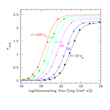
Figure 1: Thomson thickness of the hot skin as a function of the illuminating flux and disk radius computed using the code of Życki & Różańska (2001). Fitting formula (Eq. 9) has been used as a representation of the results (curves) for a given value of the spectral index of illuminating radiation. Power law with $\Gamma=1.65$ was used in the presented case.

Knowing $\tau_{\rm hot}$ we estimate the effective amplitude of the cold reprocessed component as

$$R={[p_{\rm tr}(\tau_{\rm hot})]^{2}\over 1+p_{\rm rf}(\tau_{\rm hot})},$$ (10)

where $p_{\rm tr}(\tau_{\rm hot})$ is the probability of an illuminating photon being transmitted through the hot skin to the cold disc, while $p_{\rm rf}(\tau_{\rm hot})=1-p_{\rm tr}(\tau_{\rm hot})$ is the probability of the photon being back-scattered in the hot skin and contributing to the primary continuum (Życki & Różańska 2001). The square of $p_{\rm tr}$ in the numerator comes from the fact that the reflected photons have to go twice through the hot skin. The probabilities are estimated using a Monte Carlo code for a purely scattering atmosphere. The above prescription for $R$ is obviously rather approximate, so we do not attempt to e.g. reproduce the correct observed amplitude of the reprocessed component. The function $S(\tau_{\rm hot})$ describing the dependence of the soft flux from thermalization on $\tau_{\rm hot}$ (see Eq. 3) is taken from Poutanen (2002),

$$S(\tau_{\rm hot})=(1-a){7+\exp(-10\tau_{\rm hot})\over 2[4+3\tau_{\rm hot}(1-a)]},$$ (11)

where $a$ is the cold reflection albedo, $a\approx 0.2$.

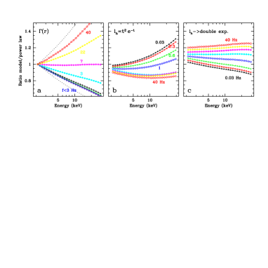
Figure 2: Test cases of Fourier-$f$ resolved spectra, plotted as ratio to $E^{-1.75}$ power law. Panel (a) shows an artificial case of a power law dependence of $\Gamma(r)$ such that $\Gamma(r_{\rm min})=1.5$ while $\Gamma(r_{\rm max})=2$, i.e. the shorter flares have harder spectra. The dotted lines show the limiting functions $E^{-1.5}$ and $E^{-2}$. Labels denote the Fourier frequency with the $f<3$ denoting: 1, 0.6, 0.3 and 0.03 Hz. The frequencies in all panels are the same. Panels (b) and (c) show the model of PF99 (i.e. no radial dependence of flares’ parameters, with spectral evolution during flares), for the PF99 and double exponential heating functions, respectively (see eq. 1 and 2). Spectra were rescaled for clarity. Note opposite behaviour of the spectra for the two $l_{\rm h}(t)$, and no dependence on $f$ in the range $f>3$ Hz, where the PSD is formed by superposition of individual flares.

The spectrum of the reprocessed component is constructed according to the simple formula of Lightman & White (1988),

$$S_{\rm refl}(E)={1-\epsilon\over 1+\epsilon}S_{\rm prim}(E),\quad\quad\epsilon=\sqrt{{\kappa_{\rm abs}\over\kappa_{\rm abs}+\kappa_{\rm es}}},$$ (12)

where $\kappa_{\rm abs}(E)$ and $\kappa_{\rm es}(E)$ are the photo-absorption and electron scattering opacities, respectively. “Cold” matter absorption opacities and elements abundances from Morrison & McCammon (1983) are used. Eq. 12 gives the angle averaged reflected spectrum and it is valid up to $\sim 15$ keV, i.e. as long as the electron scattering can be treated as elastic. Formula (12) is multiplied by a simple exponential cutoff to mimic the proper shape of the reflected continuum at higher energies. This rough approximation to the reflected spectrum is sufficient for our purposes, since the spectra only up to $\sim 30$ keV will be presented, and it is not feasible to use e.g. the proper angle-dependent functions of Magdziarz & Zdziarski (1995). The Fe K_α line is added to the reprocessed continuum. Its equivalent width (EW) is computed as a function of the spectral slope, $\Gamma$, based on computations by Życki & Czerny (1994). We note a number of simplifications involved in the above treatment of the reprocessing: most importantly, constant $\Gamma$ was used in computing $\tau_{\rm hot}$, while the continuum slope evolves during a flare. Furthermore, in our basic model no time delay is assumed in computing the reprocessed component, either due to finite light travel time or adjustment of hydrostatic equilibrium (Nayakshin & Kazanas 2001). However, a possible influence of the latter effect on the results will be presented in Sec. 4.3.3 in a very simple approximation.

Finally, the $f$-resolved spectra are computed according to the prescription given by Revnivtsev et al. (1999). The normalized power spectral density (PSD) is computed as,

$$P_{j}=2{T\over\bar{C}^{2}}|C_{j}|^{2},\quad\quad j=0,\dots,N-1$$ (13)

$$C_{j}=\sum_{k=0}^{N-1}\,c_{k}\,e^{2\pi if_{j}t_{k}},$$ (14)

where the discrete frequencies $f_{j}\equiv j/T$ for $j=-N/2,\dots,N/2$; $T$ is the total light curve time, $\bar{C}$ is the mean count rate, while $c_{k}$ are the number of counts in $k$-th time bin. The $f$-resolved spectrum at energy $E_{i}$ and Fourier frequency $f_{j}$ is then defined as

$$S(E_{i},f_{j})=\bar{C}_{i}\sqrt{P_{i}(f_{j})\,\Delta f_{j}}=\sqrt{{2|C_{i,j}|^{2}\over T}\Delta f_{j}}.$$ (15)

All computations are done for the central black hole mass $M=10\,{\rm M}_{\odot}$, accretion rate ${\dot{M}}=0.01{\dot{M}}_{\rm Edd}$, where ${\dot{M}}_{\rm Edd}=L_{\rm Edd}/(\varepsilon c^{2})$ and $\varepsilon=0.057$ is the accretion efficiency. A fraction $\xi=0.2$ of total gravitational energy is assumed to be dissipated in the disc, with the rest converted to hard X–rays (e.g. Di Salvo et al. 2001).

3 Test runs

Before presenting the results of the full model computations let us consider simpler test runs, which turn out to be helpful in understanding the interpretation of the Fourier-$f$ resolved spectra.

The first, trivial test run is to assume that (1) there is no spectral evolution during a flare, i.e. the feedback between the soft and hard X–rays is switched off, and (2) all flares have the same spectra (no radial dependence of any of the parameters). The reprocessed component is not computed. All frequency-resolved spectra are then expected to be the same and equal to the assumed spectrum, as is indeed the case in our computations.

Second, we set up a run with an artificial dependence of spectrum on the flare time scale, $\tau$, but still no spectral evolution during flares. Specifically, we assume a power law $\Gamma(\tau)$ function such, that the shortest flares (i.e. located at $r=r_{\rm min}$) have hard spectra, $\Gamma=1.5$, while the longest ones (at $r=r_{\rm max}$) have $\Gamma=2$. The reprocessed component is not computed. Result plotted in Figure 2a show, as expected, the high frequency spectra are hard and the spectra soften with decreasing $f$. Below $f\approx 3$ Hz, where PSD is formed by flares’ avalanches, the slope of the energy spectra is no longer dependent on $f$.

Third, we introduce spectral evolution during flares, but neither the radial dependences nor reprocessing. The model is thus equivalent to that of PF99, with the same values of all parameters, $\lambda=45$; $\mu=0.8$; $\alpha=7$; $p=1$; $\tau_{\rm min}=1$ ms; $\tau_{\rm max}=0.15$ s, $H_{0}=0.5$, $D_{0}=0.5$. The frequency-resolved spectra now too show some Fourier frequency dependence, even though all flares have the same time evolution (in time units of $\tau$). In Fig. 2b,c the spectra are plotted for the two flare profiles (eq. 1 and eq. 2). The dependencies on $f$ are opposite for the two profiles: for the PF99 profile the spectra are harder at lower frequencies, while the opposite is true for the double exponential profile. All $f$-resolved spectra are identical in the frequency range where individual flares form the PSD, i.e. $f>3$ Hz (see fig. 2b in PF99), the latter value being related to $\tau_{\rm max}$ and chosen to match the break in observed PSD.

The opposite behaviour of energy spectra for $f<3$ Hz is related to differences in spectral evolution during a flare for the two profiles. For the PF99 profile the rise time at soft X-rays is shorter than at hard X-rays (see fig. 1b in PF99), therefore the soft X-ray PSD breaks at higher frequency than the hard X-ray PSD. The high-$f$ energy spectra are thus softer. The opposite is true for the double exponential profile: the soft X-ray rise time is longer here, the soft X-ray PSD breaks at lower $f$, and the higher-$f$ energy spectra are harder.

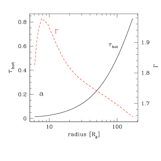
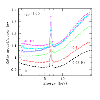
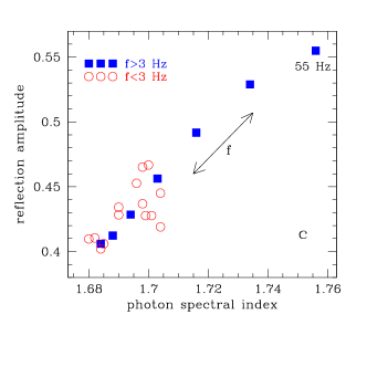
Figure 3: Results of computations for the basic model with the double exponential $l_{\rm h}(t)$ (eq. 2). Panel (a) shows the flux-average $\tau_{\rm hot}$ and $\Gamma$ as functions of radius. The hot skin is thickest at the maximum radius and, as a consequence, the spectrum is hardest there. This means that the high-$f$ spectra, originating at small $r$, are soft, reversing the trend of hardening with $f$, as shown in panel (b) – compare with Fig. 2c. The spectra plotted in panel (b) are for $f=0.03$, 0.6, 1, 3, 22 and 40 Hz, ordered by increasing normalization at 2 keV. Panel (c) plots the $R$–$\Gamma$ correlation with the Fourier frequency as the control parameter. The correlation holds only for high frequency, $f\geq 3$ Hz (solid squares), i.e. when the PSD is formed by individual flares, but it breaks down for avalanches of flares ($f<3$ Hz, empty circles). The EW of the Fe K_α line (panel d) shows a complicated behaviour: it follows the $R$–$\Gamma$ correlation for $f\geq 3$ Hz; below this frequency it is roughly constant, with a weak minimum $f\approx 1$ Hz.

4 Full model runs

The main qualitative results of the computations with the hot skin can actually be easily predicted. Assuming $R_{\rm flare}(r)={\rm const}$ and $l_{\rm h,max}(r)={\rm const}$ we obtain that the maximum illuminating flux is independent of radius. Since the gravity decreases with radius, the thickness of the hot skin will increase with radius. This is opposite to what is observed in usual computations (Nayakshin 2000; Życki & Różańska 2001), where the illuminating flux is proportional to the locally dissipated gravitational energy. Moreover, the total luminosity of a flare is proportional to its time scale, $L_{\rm flare}=\int_{0}^{T}L_{\rm flare}(t)\,dt\propto\tau$ for both flare profiles. Thus the emitted radiation is dominated by emission from outer radii (recall that by assumption $r\propto\tau^{2/3}$) of the emitting region, i.e. where the hot skin is thickest.

4.1 Basic model

In our basic model we assume the double exponential profile of the flare heating function, eq. 2, with the following parameters: $\lambda=60$, $\mu=0.7$, $\alpha=5$, $p=1$, $\tau_{\rm min}=1$ ms, $\tau_{\rm max}=0.15$ s. The value of $H_{0}$ ($\propto$vertical velocity of the flare) is such that the height of the flare above the disc is equal to its radius at the peak of energy dissipation, while $D_{0}=0.7$, so that the average spectrum has slope $\Gamma\approx 1.7$.

The full numerical simulations confirm the above qualitative estimates. The flux-weighted average thickness of the hot skin is plotted in Figure 3a, together with the average slope of the Comptonized continuum. The thickness reaches maximum at the maximum radius (recall that the existence of the maximum radius comes from the assumption of a unique relation between the flare time scale and radius). The Comptonized continuum originating at larger distances is then indeed harder. Spectral index, $\Gamma$, is smaller than in the test run (for the same values of other parameters) because of the reduction of the soft reprocessed flux due to the hot skin.

The $f$-resolved spectra are presented in Figure 3b. The high frequency, $f\geq f_{\rm break}$ ($f_{\rm break}\approx 2$ Hz), spectra are now split due to the radial dependence of $\tau_{\rm hot}$ (compare with Fig. 2c). Above $f_{\rm break}$, the higher the frequency the softer (intrinsically) the spectra and the larger the amplitude of the reprocessed component (so the hardening above $\approx 10$ keV is more significant). The $R$–$\Gamma$ correlation holds for these high Fourier frequencies, as shown in Figure 3c. The values of $R$ and $\Gamma$ plotted there at each $f$ were obtained by constructing an e.g. “$\Gamma$-spectrum”, $S(\Gamma,t)=l_{\rm h}(t)\times G[\Gamma-\Gamma_{0}(t)]$ at each point in time, where $G(x)$ is a (narrow) gaussian function and $\Gamma_{0}$ is the current value of the spectral index. The $\Gamma$-spectrum thus describes the current distribution of the spectral index, analogously to the energy spectrum describing the distribution of energy. Obviously, since $\Gamma$ has a well defined value at each time step, its distribution is strictly speaking a Dirac $\delta$-function. Thus obtained sequence of spectra can be analyzed analogously to the usual energy spectra. In particular $f$-resolved $\Gamma$-spectra were found, and the mean values of $\Gamma$ and $R$ from these latter spectra are plotted in Fig. 3c. An alternative procedure of determining $\Gamma$ and $R$ for each $f$ would be to fit a reflection model to a spectrum for a particular Fourier component. The result would however be dependent on the reflection model used, hence the above, model independent procedure was adopted. Variation of $\Gamma$ below $f\approx 3$ Hz is due to spectral evolution during a flare (Fig. 2) rather than the presence of the hot skin and, as a consequence, the $R$–$\Gamma$ correlation does not hold for those lower frequencies. This can also be seen from Fig. 3d, where the EW of the Fe K_α line is plotted as a function of $f$. There is a clear monotonic dependence EW$(f)$ for $f\geq f_{\rm break}$, but not so below this frequency.

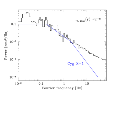
Figure 4: PSD from the 3 keV lightcurve in the model with radial dependence of $l_{\rm h,max}$: $l_{\rm h,max}(r)\propto r^{-2.5}$. The diameter of the flare is assumed constant. The radial dependence of the peak flare luminosity influences the distribution of number of events over luminosity and, consequently, affects the PSD. In this example the PSD has no high-$f$ break, which is commonly observed in black hole binary systems at $f\sim 1$ Hz.

4.2 Comparison with observations

The trends obtained in the presence of the hot skin are clearly opposite to what was found from observations of black hole binaries. For both Cyg X–1 and GX 339-4 the $f$-resolved spectra are harder when $f$ increases (Revnivtsev et al. 1999, 2001). This holds best for the frequency range $\approx 0.5$–$12$ Hz, where both single flares and flares’ avalanches form the PSD. The $\Gamma(f)$ dependence seems to flatten both at low, $f<0.5$ Hz, and high, $f>10$ Hz, frequencies (Revnivtsev et al. 1999). Similar conclusion, that the shots contributing to low-$f$ part of PSD have softer spectra than average, was reached by Negoro, Kitamoto & Mineshige (2001), using the technique of superposed shots profile. The EW of the Fe K_α line decreases monotonically with $f$ for $f>0.5$ Hz, being $\sim$constant below that frequency (Revnivtsev et al. 1999, 2001). Again this is incompatible with the model, where a rise of EW with $f$, for $f>1$ Hz is observed. At low frequency, $f<1$ Hz, the model EW$(f)$ is $\sim$constant at $\approx 40$ eV, i.e. the reflection is least efficient. The observed value is $\approx 100$ eV, compatible with amplitude of reflection $R\approx 1$ (Revnivtsev et al. 1999).

4.3 Variations on the basic model

4.3.1 Radial dependence of the flare peak luminosity

From the discussion above it is clear that the opposite behaviour of Comptonized spectra with Fourier frequency to that observed is partly due to the peak flares luminosity being constant with radius. Additionaly, the increase of luminosity with radius is obviously in disagreement with the radial dependence of the gravitational energy release, $dL/dr(r)\propto rr^{-3}$. It might therefore seem appropriate to modify the $l_{\rm h,max}(r)$ dependence assuming it should decrease with radius, so that the longer flares have lower peak luminosities. However, any such modification will affect the PSD. This is because the PSD is related to the distribution of the number of events (individual flares and avalanches) over their (total) luminosity. The $f^{-1}$ behaviour is a direct result of superposing many small events, fewer bigger events, still fewer even bigger events, etc. (e.g. Bak 1997). The break at $f\approx 2$ Hz in PSD in the original model of PF99 seems to be related to a break in the distribution $dN/dL$ in this model which occurs at $L=\tau_{\rm max}l_{\rm h,max}\times 2R_{\rm flare}m_{\rm e}c^{2}/\sigma_{\rm T}$ (i.e. total luminosity of longest flares). Decreasing $l_{\rm h,max}$ at the maximum radius (i.e. longest flares) decreases the range of $L$ spanned by individual flares. The resulting distribution has no clear break and, as a result, the PSD has no break in the whole range of frequencies of interest (Fig. 4). This is obviously incompatible with the observed PSD of X–ray lightcurves, which universally show breaks at a few Hz. The conclusion about lack of break in PSD seems to be independent of the value of the exponent in the $P(\tau)$ probability (see Sec. 2.1), provided that $l_{\rm h,max}(r)$ is adjusted to give an assumed $dL/dr(r)$ (e.g. $\propto r^{-2}$) dependence. Since the total emission from each flare is $\propto\tau l_{\rm h,max}$, the radial distribution of emission is $dL/dr\propto dN/d\tau\times\tau l_{\rm h,max}\propto P(\tau)\tau l_{\rm h,max}$. For the assumed $P(\tau)\propto\tau^{-1}$ and $\tau(r)\propto r^{3/2}$ (Eq. 4), the distribution becomes $dL/dr\propto r^{1/2}l_{\rm h,max}(r)$. The PSD plotted in Fig. 4 was computed assuming $l_{\rm h,max}(r)\propto r^{-2.5}$, which gives $dL/dr(r)\propto r^{-2}$.

The effect of the hot skin in this model is insignificant. This is because, adjusting the normalization of $l_{\rm h,max}(r)$ so that the mean luminosity-weighted $l_{\rm h}\approx 10$, the simple time average of $l_{\rm h}$ is much smaller than before. This requires larger sizes of flares, $R_{\rm flare}$, in order for the total luminosity to remain constant. Hence, the maximum illuminating flux, which scales as $F\propto L_{\rm flare}/h^{2}\propto 1/R_{\rm flare}^{2}$ (assuming the height of maximum dissipation $h\approx R_{\rm flare}$), is smaller than in the model with $l_{\rm h,max}(r)={\rm const}$. As a consequence, no correlations is obtained between $R$ and $\Gamma$. The $f$-resolved spectra in this model show slight hardening with $f$, due to flare spectral evolution (see Fig. 2c), but the reprocessed component is constant with $f$.

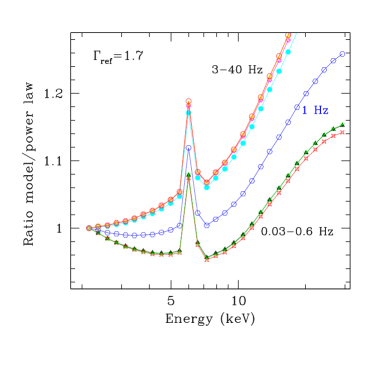
Figure 5: Fourier $f$-resolved spectra in the modified model, assuming that the location of stimulated flares is the same as their stimulating flare (Sec. 4.3.2), i.e. whole avalanche developes in the same place. The high-$f$ ($f>3$ Hz) spectra are now the same, since the correspondence of time scale and physical conditions is lost.

4.3.2 Modified radial distribution of the stimulated flares

The Fourier frequency dependence of the spectra becomes less significant, when the assumption is made that the spatial positions of all stimulated flares coincide with that of their stimulating flare (Sec 2.2; the distribution of time scales $P(\tau)\propto\tau^{-1}$ is retained for all flares). This is to be expected, since the correspondence of variability time scale (i.e. $f$) and physical conditions (i.e. $r$) is no longer unique. In particular, the high-$f$ spectra are almost identical in this case, while the lower-$f$ ones are somewhat softer compared to results of the basic model (Fig. 5). The EW of the K_α line shows no frequency dependence being approximately constant at $\approx 60$ eV.

4.3.3 Delayed response of the reflecting medium

The properties of the reprocessed component may not be always given by the instanteneous illuminating flux, as the accretion disc needs to re-adjust to the condition of hydrostatic equilibrium with changed X–ray radiation pressure and the Compton temperature (Nayakshin & Kazanas 2001). Parameters of the hot skin are thus not given by the instantaneous flux, if the flux fluctuates rapidly. The thickness of the hot skin re-adjusts on the dynamical time scale $t_{\rm response}\approx t_{\rm dyn}=\Omega_{\rm K}^{-1}$, while its temperature on the thermal time scale, which is usually much shorter (Nayakshin & Kazanas 2001). This effect may influence our results, since the response time is approximately equal the flare time scale, $\tau\approx t_{\rm dyn}\approx t_{\rm response}$. Since proper computations of time-dependent response of an accretion disc to changing illumination are not possible at present, we model here the response in a rather approximate way, motivated by the results of Nayakshin & Kazanas (2001). We simply assume that for each flare $\tau_{\rm hot}(t)$ is determined by illumination flux at an eariler time $t_{1}=t-t_{\rm response}=t-t_{\rm dyn}$, i.e. the complex response of reflection is approximated as a simple time shift. In particular, at the beginning of a flare, for $t<t_{\rm dyn}$, there is no hot skin and the reprocessed component is produced with amplitude 1.

The radial dependence of $\tau_{\rm hot}$ in this model is qualitatively the same as in the basic model, i.e. $\tau_{\rm hot}$ increases with $r$. The values of $\tau_{\rm hot}(r)$ are now smaller, though, since by assumption $\tau_{\rm hot}$ is fixed at zero for a certain time $\approx\tau$ during each flare. The radial dependence of $\Gamma$ is somewhat weaker but the overall trends are virtually the same as in our basic model (Fig. 3b). With increasing $f$ the spectra become harder first, then, above $f\approx 3$ Hz, they soften. The EW of the K_α line has the same $f$-dependence except for a slight overall increase by 15–20 eV. There results are not unexpected since the delay is relatively short compared to the duration of a flare. With increasing delay, still the same qualitative results are obtained. The influence of the hot skin becomes less significant but the radial trends are the same, if the delay time scale is related to the flare time scale. In the limit of a very long delay the presence of the hot skin becomes unimportant, and the model reduces to the original model of PF99.

5 Discussion

A number of geometrical/physical models of accretion onto compact sources can be constructed, if only a part of the available information on X-ray emission is used. Supplementing the usually employed energy spectral analysis with time variability and, in particular, correlated spectral–timing behaviour, one can attempt to distinguish between the models. In this paper predictions for Fourier-resolved spectroscopy are presented for the model of magnetic flares avalanches (PF99) above an accretion disc with hot ionized skin.

The basic model formulated by PF99 is quite successful in explaining both energy spectra and a number of timing characteristics: PSD, hard X–ray time lags and the coherence function. With the suitably chosen flare profile (e.g. a double exponential with $t_{\rm rise}\gg t_{\rm decay}$), the auto- and cross-correlation function can also be reproduced (Maccarone et al. 2000). The dependence of energy spectra on Fourier frequency, resulting from the spectral evolution during flares alone, is in agreement with observations for e.g. the double exponential flare profile, but not for the profile assumed in PF99 (Sec 3).

Our extension of the PF99 model is to assume that there exists at least partial correspondence between location of a flare and its time scale. The simplest assumption about such correspondence is that it follows from projecting the flares time scales onto the (inverse of) Keplerian frequency. The shortest flares are then located near the inner radius of the disc, the longer a flare the farther away it is located. Now, in the basic model both the peak heating rate (compactness parameter) and flare diameter are independent of radius, which means that the peak flux of the disc illuminating X–rays is independent of radius, too. Since the vertical component of gravity decreases with radius ($g_{\rm z}\propto(z/r)r^{-2}$), the thickness of the hot ionized skin increases with radius. The fast flares, located where the hot skin is thinest, have then softer spectra than the slower flares located where the thick hot skin decreases the effectiveness of thermalization of X–rays and, consequently, the flux of soft photons for Comptonization. As a result, the energy spectra corresponding to high Fourier frequencies are softer than the lower $f$ spectra, for the frequency where the properties of individual flares determine the PSD, $f>f_{\rm break}$, where $f_{\rm break}=1$–3 Hz in black hole binaries. This is opposite to the observed trends, which show steady hardening of the spectra with increasing Fourier frequency, at least up to $\approx 12$ Hz (Revnivtsev et al. 1999).

As a consequence, the properties of the reprocessed component in the presented model, in particular the Fe K_α line, do not agree with the observed trends, either. At high $f>f_{\rm break}$ the reflection amplitude and EW of the K_α line increase sharply with $f$, as a consequence of the inwards–decreasing thickness of the hot skin. At low $f<1$ Hz the model $R$ and EW of the line are roughly constant, however $R$ is significantly less than 1 and, consequently, EW is smaller than the corresponding value of $\sim 100$ eV. This is contrary to the observed $R\approx 1$ and EW$\approx 100$ eV at these low frequencies.

These results hold true even when some of the model assumptions are modified (Sec. 4.3). None of the modifications made: the different radial distribution of the stimulated flares, radial dependence of the peak flare luminosity or the delayed response of reflection, changed the trends of spectral parameters with Fourier frequency. It is worth emphasizing that the perhaps most obvious of the above modifications – the radial distribution of flares peak luminosity such that the total flares luminosity decreases with radius – not only does not help to reproduce the observed EW$(f)$ and $\Gamma(f)$, but it also changes the PSD so that it no longer agrees with observations. It remains to be seen whether a more complex formulation of the model is possible, which would simultaneously predict the correct PSD and thickness of the hot skin decreasing with radius.

The same technique of analysis of $f$-resolved spectra can be applied to other models mentioned in Sec. 1. In the dynamic corona model with bulk outflow of the plasma, the plasma velocity, $\beta$, is the control parameter of the $R$–$\Gamma$ correlation (Beloborodov 1999a,b). The observed $f$-dependence of the energy spectra would require higher $\beta$ closer to the center. This is indeed expected, if the X-ray luminosity scales with local gravitational energy dissipation. However, if the X–ray emission is determined from the properties of the flares, assuming their radial distribution as adopted in this paper (Sec. 2.2, Eq. 4), then stronger X–ray emission is expected from larger distances, exactly as in the computations of the hot skin model. It is then likely that $\beta$ will increase with radius, analogously to the result that the thickness of the hot skin increases with radius in our model. The result for the $f$-resolved spectra will then be the same as for the model with hot skin. In the alternative geometry (the optically thick flow distrupted at certain radius and replaced with some form of hot optically thin flow), the model of Böttcher & Liang (1999) can be used to compute the $f$-resolved spectra. Alternatively, the idea of Kotov, Churazov & Gilfanov (2001; see also Nowak et al. 1999), that the X–ray emitting perturbations are propagating inwards, if developed further into a more physical model, could be used to predict the $f$-resolved spectra.

6 Conclusions

• Fourier-resolved X–ray spectroscopy is a powerful tool for discriminating various models of accretion.

• The model of (avalanches of) magnetic flares, radially distributed above an accretion disc with hot ionized skin, predicts dependencies of various spectral parameters ($\Gamma$, $R$, EW of the Fe K_α line) on Fourier frequency opposite to those observed.

References

- [] Bak P., 1997, How Nature works, Oxford University Press, Oxford.
- [] Beloborodov A. M., 1999a, ApJ, 510, L123
- [] Beloborodov A. M., 1999b, in Poutanen J., Svensson R. eds, ASP Conf. Ser. 161, High Energy Processes in Accreting Black Holes, 295, (astro-ph/9901108)
- [] Böttcher M., Liang E. P., 1999, ApJ, 511, L37
- [] Collin-Souffrin S., Czerny B., Dumont A.-M., Życki P. T., 1996, A&A, 314, 393
- [] Coppi P. S., 1999, in Poutanen J., Svensson R., eds, ASP Conf Ser. Vol. 161. Astron. Soc. Pac., San Francisco, p. 375 (astro-ph/9903158)
- [1] Di Salvo T., Done C., Życki P. T., Burderi L., Robba N. R., 2001, ApJ, 547, 1024
- [] Esin A. A., McClintock J. E., Narayan R., 1997, ApJ, 489, 865
- [] Field G. B., 1965, ApJ, 142, 531
- [] Gilfanov M., Churazov E., Revnivtsev M., 1999, A&A, 352, 182
- [] Gilfanov M., Churazov E., Revnivtsev M., 2000a, in Proc. of the 5th Sino-German Workshop on Astrophysics, SGSC Conference Ser., Vol. 1, China Science & Technology Press, Beijing, p. 114 (astro-ph/0002415)
- [] Gilfanov M., Churazov E., Revnivtsev M., 2000b, MNRAS, 316, 923
- [] Janiuk A., Czerny B., Życki P., 2000, MNRAS, 318, 180
- [] Kazanas D., Hua X. M., Titarchuk L., 1997, ApJ, 480, 735
- [] Kotov O., Churazov E., Gilfanov M., 2001, MNRAS, 327, 799
- [] Krolik J. H., McKee C. F., Tarter C. B., 1981, ApJ, 249, 422
- [] Kuncic Z., Celotti A., Rees M. J., 1997, MNRAS, 284, 717
- [] Lehto H. J., 1989, in The 23rd ESLAB Symposium on Two Topics in X–Ray Astronomy. Volume 1: X Ray Binaries, ESA, p. 499
- [] Lightman A. P., White T. R., 1988, ApJ, 335, L57
- [] Lochner J. C., Swank J. H., Szymkowiak A. E., 1991 ApJ, 376, 295
- [] Lubiński P., Zdziarski A. A., 2001, MNRAS, 323, L37
- [] Maccarone T. J., Coppi P. S., Poutanen J., 2000, ApJ, 537, L107
- [] Magdziarz P., Zdziarski A. A., 1995, MNRAS, 273, 837
- [] Malzac J., 2001, MNRAS, 325, 1625
- [] Malzac J., Beloborodov A. M., Poutanen J., 2001, MNRAS, 326, 417
- [] Merloni A., Fabian A. C., 2001, MNRAS, 328, 958
- [] Miyamoto S., Kitamoto S., 1989, Nat, 342, 773
- [] Morrison R., McCammon D., 1983, ApJ, 270, 119
- [] Nayakshin S., 2000, ApJ, 534, 718
- [] Nayakshin S., Kazanas D., 2001, ApJ, in press (astro-ph/0106450)
- [] Nayakshin S., Kazanas D., Kallman T. R., 2000, ApJ, 537, 833
- [] Negoro H., Kitamoto S, Mineshige S., 2001, ApJ, 554, 528
- [] Nowak M. A., Wilms J., Vaughan B. A., Dove J. B, Begelman M. C., 1999, ApJ, 515, 726
- [] Poutanen J., 1998, in Abramowicz M. A., Björnsson G., Pringle J. E., eds, Theory of Black Hole Accretion Discs. CUP, Cambridge, p. 100 (astro-ph/9805025)
- [] Poutanen J., 2001, AdSpR, 28, 267 (astro-ph/0102325)
- [] Poutanen J., 2002, MNRAS, in press (astro-ph/0106189)
- [] Poutanen J., Fabian A. C., 1999, MNRAS, 306, L31 (PF99)
- [] Poutanen J., Krolik J. H., Ryde F., 1997, MNRAS, 292, L21
- [] Rees M., 1987, MNRAS, 228, 47P
- [] Revnivtsev M., Gilfanov M., Churazov E., 1999, A&A, 347, L23
- [] Revnivtsev M., Gilfanov M., Churazov E., 2001, A&A, 380, 520
- [] Różańska A., 1999, MNRAS, 308, 751
- [] Różańska A., Czerny B., 1996, Acta Astron., 46, 233
- [] Różańska A., Czerny B., 2000, A&A, 360, 1170
- [] Shakura N. I., Sunyaev R. A., 1973, A&A, 24, 337
- [] Stern B. E., Svensson R., 1996, ApJ, 469, L109
- [] Zdziarski A. A., Johnson W. N., Magdziarz P., 1996 ApJ, 283, 193
- [] Zdziarski A. A., Lubiński P., Smith D. A., 1999, MNRAS, 303, L11
- [] Życki P. T., Czerny B., 1994, MNRAS, 266, 653
- [] Życki P. T., Różańska A., 2001, MNRAS, 325, 197
- [] Życki P. T., Done C., Smith D. A., 1998, ApJ, 496, L25