Photometric redshifts from evolutionary synthesis with PÉGASE: the code Z-PEG and the $z=0$ age constraint

Photometric redshifts are estimated on the basis of template scenarios with the help of the code Z-PEG, an extension of the galaxy evolution model PÉGASE.2 and available on the PÉGASE web site. The spectral energy distribution (SED) templates are computed for nine spectral types including starburst, irregular, spiral and elliptical. Dust, extinction and metal effects are coherently taken into account, depending on evolution scenarios. The sensitivity of results to adding near-infrared colors and IGM absorption is analyzed. A comparison with results of other models without evolution measures the evolution factor which systematically increases the estimated photometric redshift values by $\Delta z\geq 0.2$ for $z>1.5$. Moreover we systematically check that the evolution scenarios match observational standard templates of nearby galaxies, implying an age constraint of the stellar population at $z=0$ for each type. The respect of this constraint makes it possible to significantly improve the accuracy of photometric redshifts by decreasing the well-known degeneracy problem. The method is applied to the HDF-N sample (see in Fernández-Soto et al.,1999). From fits on SED templates by a $\chi^{2}$-minimization procedure, not only is the photometric redshift derived but also the corresponding spectral type and the formation redshift $z_{\textrm{for}}$ when stars first formed. Early epochs of galaxy formation $z>5$ are found from this new method and results are compared to faint galaxy count interpretations. The new tool is available at: http://www.iap.fr/pegase

1 Introduction

The determination of galaxy distances is so crucial for clues on galaxy evolution and cosmic structures that a large variety of methods is currently being explored. Spectroscopic determinations are the most precise but they consume excessive observing time for deeper and deeper large galaxy samples. For instance, the redshift surveys such as CFRS(Le Fèvre (1995)), 2dF Folkes et al. (1999)), Hawaii(Cowie et al. (1994)) and more recently the SLOAN, with millions of targets with various spectral types, are complete to $z\leq 1.5$. At higher redshifts $z>1.5$, the galaxy populations observed at faint magnitudes in deep surveys cover a large range of redshifts which will be easily accessible from photometry. However many problems of degeneracy, number and width of filters and extinction first have to be clarified. Typical SED features like the 4000Å discontinuity or the Lyman break are known to be fruitful signatures for evaluation of redshifts when compared with template SEDs. Steidel et al. (1999) proposed an empirical method based on these discontinuities to detect $z\geq 4$ galaxies. Successful in discovering distant sources, the method is however imprecise and prone to degeneracies. The comparison of observed SEDs with calibrated templates on an extended wavelength range is the best way to rapidly determine redshifts of a large number of faint galaxies, on a continuous range $0\leq z\leq 4$ . Such comparisons were proposed with templates from no-evolution models by Baum (1962), Koo (1985), Loh & Spillar (1986) and more recently Fernández-Soto et al. (1999) (hereafter FSLY); others proposed evolutionary SED methods such as Bolzonella et al. (2000) and Massarotti et al. (2001a) using templates derived from a variety of evolutionary codes. However the evolutionary codes and their applications may differ. If results are roughly similar at low redshifts (see Leitherer et al. (1996)), they may actually strongly differ from each other at high redshifts, depending on adopted star formation laws and the corresponding age constraints, initial mass function, dust and metal effects as well as interpolation algorithms.

An essential property of most codes is the large wavelength coverage from the far-UV to the near-infrared needed to compute SEDs that are highly redshifted. Moreover our code PÉGASE.2, Fioc & Rocca-Volmerange (1997), in its current version (see next footnote) is able to take into account metallicity effects in its stellar library and isochrones. Evolution scenarios of nine spectral types, defined by star formation parameters, have been selected to reproduce the observed statistical SEDs of $z=0$  galaxy templates, Fioc & Rocca-Volmerange (1999b). Then two correction factors (cosmological k-correction and evolutionary e-correction) are computed with the model to predict redshifted SEDs, in order to be used as comparison templates to observations. Other PEGASE.2 scenarios based on different prescriptions of dust properties or star formation parameters might be computed and used as templates only if they respect fits of $z\simeq 0$ galaxy properties. This is beyond the objectives of this paper. Another method of photometric redshift determination supposes that the evolution effect is dominated by shot noise, Connolly et al. (1995).

We present in section 2 a new tool, Z-PEG, to estimate photometric redshifts on a continuous redshift range $0\leq z\leq 6$ or more. Observed colors or spectra are statistically compared to the PÉGASE.2 atlas for 9 spectral types (starburst: SB, irregular: Im, spiral: Sd, Sc, Sbc, Sb, Sa, SO and elliptical: Ell galaxies). Section 3 presents the results for the well-known Hubble Deep Field North and the comparison with spectroscopic redshifts allows us to derive average values of evolution factors. Section 4 shows the sensitivity to various parameters such as the NIR colors and IGM absorption. Interesting consequences for the redshifts of formation of the sample are derived in section 5. Discussion and conclusions are proposed in sections 6 and 7 respectively.

2 The code Z-PEG (web available)

2.1 The evolution scenarios of galaxies

The atlas of synthetic galaxies used as templates is computed with PÉGASE.2 on the basis of evolution scenarios of star formation. The synthesis method assumes that distant galaxies are similar to nearby galaxies, but look younger at high $z$ since they are seen at more remote epochs. Respecting this constraint will make our redshift determinations more robust. In an earlier paper (Fioc & Rocca-Volmerange (1997)), we investigated the selection of star formation rates able to reproduce the multi spectral stellar energy distributions of nearby galaxies. Another article by Fioc & Rocca-Volmerange (1999b) computed the statistical SEDs of about 800 nearby galaxies observed from the optical and the near-infrared for eight spectral types of galaxies and used to fit scenarios at $z$=0. Star formation rates (SFRs) are proportional to the gas density (with one exception, see table 1), the astration rate $\nu$ increasing from irregular Im to elliptical E galaxies. The star formation rate of starburst SB scenario is instantaneous. Infall and galactic winds are typical gaseous exchanges with the interstellar medium. They aim to simulate the mass growth and to subtract the gas fraction (preventing any further star formation) respectively. Unlike other studies (Fernández-Soto et al. (2001a), Massarotti et al. (2001b)), our scenarios do not need to add any starburst component to be consistent with $z\simeq 0$ observations.

Table 1: PEGASE.2 scenarios used as template parameters. SFR=$\nu\times M_{\textrm{gas}}$, except for starbursts and irregular galaxies. $\nu$  is in units of $\textrm{Gyr}^{-1}$  and M${}_{\textrm{gas}}$  is the gas density. Infall time-scales are in Myrs. The dust distribution is fitted on a King profile for E and S0, while an inclinaison-averaged disk distribution is applied to spiral and irregular galaxies (see text for details). Starburst galaxies have no extinction correction. For all the scenarios, the age of the universe is an upper limit on the age.

Type	$\nu$	infall	gal. winds	age at $z=0$
SB	$\delta(t)$			1 Myr to 2 Gyr
E	3.33	300	1 Gyr	$>13$ Gyr
S0	2	100	5 Gyr	$>13$ Gyr
Sa	0.71	2 800		$>13$ Gyr
Sb	0.4	3 500		$>13$ Gyr
Sbc	0.175	6 000		$>13$ Gyr
Sc	0.1	8 000		$>13$ Gyr
Sd	0.07	8 000		$>13$ Gyr
Im	0.065	8 000		$>9$ Gyr

The initial mass function (IMF) (Rana & Basu (1992)), is used in our evolution scenarios. However Giallongo et al. (1998) showed that the choice of the IMF does not influence much the photometric redshift estimates of high-$z$  candidates ($z>2.5$).
PÉGASE.2 is the most recent version of PÉGASE, available by ftp and on a web site. Non-solar metallicities are implemented in stellar tracks and spectra but also a far-UV spectral library for hot stars (Clegg & Middlemass (1987)) complements the Lejeune et al. (1997, 1998) library. The metal enrichment is followed through the successive generations of stars and is taken into account for spectra of the stellar library as well as for isochrones. In PÉGASE.2, a consistent treatment of the internal extinction is proposed by fitting the dust amount on metal abundances. The extinction factor depends on the respective spatial distribution of dust and stars as well as on its composition. Two patterns are modeled with either the geometry of bulges for elliptical galaxies or disks for spiral galaxies. In elliptical galaxies, the dust distribution follows a King’s profile. The density of dust is described as a power of the density of stars (see Fioc & Rocca-Volmerange (1997) for details). Through such a geometry, light scattering by dust is computed using a transfer model, outputs of which are tabulated in one input-data file of the model PÉGASE. For spirals and irregulars, dust is distributed along a uniform plane-parallel slab and mixed with gas. As a direct consequence, the synthetic templates used to determine photometric redshifts at any $z$, as well as to fit the observational standards at $z=0$, are systematically reddened. We also add the IGM absorption following Madau (1995) on the hypothesis of Ly_α, Ly_β, Ly_γ and Ly_δ line blanketing induced by H i clouds, Poisson-distributed along the line of sight. This line blanketing can be expressed for each order of the Lyman series by an effective optical depth $\tau_{\textrm{\small eff}}=A_{i}\times(\lambda_{\textrm{\small obs}}/\lambda_{i})^{1+\gamma}$, with $\gamma=2.46$ and $\lambda_{i}=1216,1026,973,950$ Å  for Ly_α, Ly_β, Ly_γ and Ly_δ respectively. The values of $A_{i}$ are taken from Madau et al. (1996), in agreement with the Press et al. (1993) analysis on a sample of 29 quasars at $z>3$. We shall see below that the IGM absorption alters the visible and IR colors more than about $0.1$ mag as soon as $z>2$, leading to a more accurate determination of photometric redshifts at these distances.
For each spectral type, a typical age of the stellar population is derived. Time scales, characteristics and ages of the scenarios are listed in table 1.

2.2 The $\chi^{2}$ minimization procedure

A 3D-subspace of parameters (age, redshift, type) is defined by the template sets. It is used to automatically fit observational data. This subspace in the age–redshift plane is limited by the cosmology in order to avoid inconsistencies: a 10 Gyr old galaxy at $z=2$  cannot exist in the standard cosmology because at this redshift, the age of the universe is about 5 Gyr. Moreover the subspace is also limited by the age (redshift corrected) imposed by the adopted scenario of spectral type evolution. As an example, if elliptical and spiral galaxies must be at least 13 Gyr old at $z=0$, it means at least 5 Gyr at $z=1$ and so on.
Each point is granted a synthetic spectrum; its flux through the filter $i$ is called $F^{synth}_{i}$. For each point of this 3D-subspace, the fourth parameter $\alpha$ is computed with a $\chi^{2}$ minimization to fit as well as possible the observed fluxes in filters:

$$\chi^{2}=\sum_{i=1}^{\it N}\left[\frac{F^{obs}_{i}-\alpha\times F^{synth}_{i}}{\sigma_{i}}\right]^{2}$$ (1)

$N$ is the number of filters, $F^{obs}_{i}$  and $\sigma_{i}$  are the observed flux and its error bar through the filter $i$ respectively. In the case of an observed spectrum without redshift signatures, the sum can also be computed from wavelength bins. Then, each point of the 3D-subspace of parameters has a $\chi^{2}$ value. A projection of this 3D-$\chi^{2}$ array on the redshift dimension gives the photometric redshift value $z_{\textrm{\tiny phot}}$.

The values of $\sigma_{i}^{2}$ can be evaluated by the quadratic sum of the systematic errors and of the statistical errors. The extremely low values of observational errors, adopted as statistical, may result in anomalously high reduced $\chi^{2}$ minima. In this study we consider as negligible systematic errors, keeping in mind that it maximizes the $\chi^{2}$ minimum value (possibly up to 100). In such a case, statistical rules claim that the result (the photometric redshift) is not reliable and has to be excluded. Yet, with such prescriptions, most of the results would be excluded, because the photometric errors of the observations are very low. This is why all the primary solutions are often kept, including cases of very high reduced $\chi^{2}$ minima. In the following, we will also adopt this philosophy. However, our error bars might appear larger than in the previous studies, that limit their results to one unique but less robust solution. Indeed, the estimation of the error bar of a photometric redshift is often estimated by the redshifts for which $\chi^{2}\leq\chi^{2}_{\textrm{ \tiny min}}+1$. This method is only valid when the minimum reduced $\chi_{r,\textrm{\tiny min}}^{2}\simeq 1$ (otherwise the error bar is very underestimated).
We choose to estimate the error bar by the redshift values for which $\chi_{n}^{2}\leq\chi^{2}_{n,\textrm{\tiny min}}+1$, where $\chi_{n}^{2}$ is the $\chi^{2}$ “normalized” with $\chi^{2}_{r,\textrm{\tiny min}}=1$ . The error bar is then much larger and may lead to secondary solutions. Fernández-Soto et al. (2001b) use another accurate estimation of the error bars which also gives secondary solutions, for the $3\leavevmode\nobreak\ \sigma$ level for instance. This is the case when the Lyman and Balmer breaks are hardly distinguished, as an example.

2.3 The Z-PEG interface

Z-PEG is an interface available on the PÉGASE web site (see footnote on page 2). Inputs are fluxes or colors of the observed galaxies and their error bars. Sets of classical filters defined in a variety of photometric systems are proposed. It is possible to use a user-defined filter, with its passband and calibration. In the general case, for which no information on the galaxy spectral type is a priori known, the minimization procedure is tested on all the template types. It is also possible to restrain the template galaxies to a given type. Types are then chosen among the 9 pre-computed synthetic spectra. The default redshift sampling is $0.25$ and may be reduced on a narrower redshift range. The age and redshift axes are respectively defined by step - up and - down limits. The user will choose the cosmological parameters ($H_{0}$, $\Omega_{M}$, $\Omega_{\Lambda}$), on which the time-redshift relation depends. The default values of cosmological parameters are those adopted in this article.

Outputs are the estimated photometric redshift $z_{\textrm{\tiny phot}}$ and its error bar, the age and the spectral type of the best fitted synthetic galaxy. A $\chi^{2}$ projection map in the age–redshift plane and its projection on the redshift and age axes (see Fig. 1) are also presented.

2.4 The coherency test

The relevance of the fit procedure is checked on a synthetic galaxy of the atlas with a known $z$. As an example, input data are the colors computed from the SED of the Sbc galaxy at age 5 Gyr and redshift $z=0.989$. The output value is, as expected, $z=0.99$, identical to the input galaxy redshift ($z=0.989$) with a precision of $\Delta z=0.01$ (no photometric error). Figure 1 shows the resulting projected $\chi^{2}$ map on the age $vs$ redshift plane for this test.

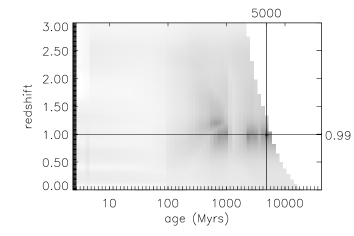
Figure 1: The test of coherency on the $z=0.989$ and $5$ Gyr old galaxy: darker grey zones correspond to lower $\chi^{2}$ values in the age – z plane. The minimum $\chi^{2}$ location is the cross center of the two solid lines. The plot log${}_{\textrm{\tiny 10}}$($\chi^{2}$) versus redshift estimates the accuracy of the minimum and shows possible secondary minima.

3 Photometric redshifts with evolution

3.1 The HDF-N galaxy sample

The Hubble Deep Field North (HDF-N) catalog (Williams et al. (1996)) was chosen to test the evolution factor. Spectroscopic redshifts were measured carefully by Cohen et al. (2000), with some additions and corrections in Cohen (2001). FSLY give photometric data for the HDF-N objects and Fernández-Soto et al. (2001a) give a correspondence between their objects and the objects in Cohen et al. (2000). We exclude from the sample galaxies with negative fluxes. The remaining selected sub-sample contains 136 galaxies with redshifts distributed from $0$ to $5.6$.
The HDF-N sample presents a series of advantages to explore the accuracy of our method and to compare it to others. With a large redshift range ($0\leq z\leq 5.6$), the sample data acquired with the WFPC2/HST camera is one of the deepest (down to B=29) with an extent over the wavelength range from about 3000Å to 8000Å  with the filters F300W, F450W, F606W, and F814W (hereafter called U,B,V,I). Moreover the near-infrared standard Johnson-Cousins J, H and K_s (hereafter K) colors listed in FSLY from Dickinson (1998) were observed at the KPNO/4m telescope. The calibration used is AB magnitudes.

$$m_{\mathrm{AB}}=-2.5\log_{10}\frac{\displaystyle{\int F_{\nu}\,T_{\nu}\,\mathrm{d}\nu}}{\displaystyle{\int T_{\nu}\,\mathrm{d}\nu}}-48.60$$

with $F_{\nu}$ in erg.s^-1.cm^-2.Hz^-1. $T_{\nu}$ is the transmission of the filter.

A further advantage is the benefit of spectroscopic redshifts of the selected sub-sample, as given by Cohen (2001). This allows a statistical comparison with our photometric redshifts and an estimation of the dispersion. Another advantage of this sample is the possibility of measuring the type-dependent evolution factor by comparing our results with the FSLY ’s results, since the latter authors propose photometric redshift determinations based on a maximum likelihood analysis and 4 spectral types without any evolution effect.

3.2 The spectroscopic-$z$ – photometric-$z$  plane

Figure 2 presents the plane $z_{\textrm{\tiny spe}}$ – $z_{\textrm{\tiny phot}}$  resulting from our fit of the HDF-N sample with PÉGASE templates.

Figure 2: Comparison of photometric redshifts (points with error bars) predicted by the model Z-PEG.1 to spectroscopic redshifts of the selected HDF-N sample. The solid line of slope=1 shows the case of equality for comparison. The dotted line is the linear regression of our photometric redshifts if we exclude the points with $|z_{\textrm{\tiny ZPEG}}-z_{\textrm{\tiny spe}}|\geq 1$. Predictions are computed with IGM absorption from Madau et al. (1996) and ISM reddening according to PÉGASE algorithms. When two solutions or more are found (degeneracy), the error bars are linked by a dotted line. The squares are objects with discordant redshifts also pointed out by Fernández-Soto et al. (2001a).

3.3 Evolution factors

3.3.1 Average evolution factor on $z_{\textrm{\small phot}}$

We compare our best results $z_{\textrm{\tiny ZPEG}}$, from the evolutionary model Z-PEG.1 (selected from the variety of models in table 2) to photometric redshifts $z_{\textrm{\tiny FS}}$ estimated by FSLY . These authors only took into account k-corrections of the galaxy spectral distributions from Coleman et al. (1980) while we simultaneously compute the k- and e- correction factors at any $z$. Figure 3 shows the difference for each galaxy of the sample. Lines trace the median values of the difference of $z_{\textrm{\tiny FS}}$ with Z-PEG.1, and $z_{\textrm{\tiny spe}}$  values respectively. The zero value (difference to $z_{\textrm{\tiny FS}}$) is plotted for comparison. A systematic effect is observed for $z\geq$1.5. The evolution effect is measured around $<z_{\textrm{\tiny ZPEG}}-z_{\textrm{\tiny FS}}>=0.2$, independent of type. The median value $<z_{\textrm{\tiny ZPEG}}-z_{\textrm{\tiny spe}}>=-0.03$  is measured and remains inside the error bars. Evolution effects are more important for distant galaxies and an appropriate evolutionary code is required for such estimates.

Figure 3: Crosses are differences $z_{\textrm{\tiny ZPEG}}-z_{\textrm{\tiny FS}}$. For $z_{\textrm{\tiny spe}}>1.5$, the evolution factor is measured by the distance between the dotted and full lines, respectively the median value $<z_{\textrm{\tiny ZPEG}}-z_{\textrm{\tiny FS}}>$ and 0. $z_{\textrm{\tiny FS}}$ are the FSLY ’s determinations. The dashed line is the median value $<z_{\textrm{\tiny spe}}-z_{\textrm{\tiny FS}}>$. For $z_{\textrm{\tiny spe}}<1.5$, the evolution factor has the same magnitude as the error bars.

3.3.2 Determination of galaxy spectral types

Our best fit gives a minimal $\chi^{2}$ for a triplet (age, redshift, type), so that we can deduce the spectral type of the observed galaxies by comparing to the SEDs of 9 different types. The comparison of types derived by Z-PEG.1 and by FSLY is shown in Fig. 4. In most cases, ’earlier type’ galaxies are found with Z-PEG.1, particularly at high redshifts. This effect is expected from evolution scenarios because, when considering only the k-correction, FSLY would find an evolved spiral galaxy when Z-PEG.1 finds a young elliptical galaxy. A better definition of the morphological properties of galaxies in the near future will help us to arrive at a conclusion.

Figure 4: Comparison of our spectral type estimates to FSLY’s. The values are ${\textrm{t}ype}_{\textrm{\it\tiny ZPEG}}-{\textrm{t}ype}_{\textrm{\tiny FS}}$ assuming the following values for the spectral types (type 0: starburst, 1: elliptical, 2: S0, 3: Sa, 4: Sb, 5: Sbc, 6: Sc, 7: Sd, 8: Im)

Table 2: The variety of Z-PEG models is tabulated with the adopted constraints (IGM absorption, near-infrared JHK filters and age). Statistical results (mean difference and dispersion) are given in last columns. A comparison to FSLY and Massarotti et al. (2001b) results is also given. The $\overline{\Delta z}$ and $\sigma$ are computed using primary and secondary solutions for Z-PEG models (see Sect. 2.2), and primary solutions only for FSLY and MIBV models.

Z-PEG Model	IGM abs.	UBVI	JHK	age constraint			$z<1.5$	all $z$	Figure
1	x	x	x	x	$\overline{\Delta z}$	$=$	$-0.0214$	$-0.0844$	2
					$\sigma_{z}$	$=$	$\mathbf{0.0980}$	$\mathbf{0.4055}$
2	x	x	x		$\overline{\Delta z}$	$=$	$0.0251$	$-0.0621$	5
					$\sigma_{z}$	$=$	$\mathbf{0.1156}$	$\mathbf{0.4441}$
3		x	x		$\overline{\Delta z}$	$=$	$0.0252$	$-0.0589$	5
					$\sigma_{z}$	$=$	$0.1156$	$0.5738$
4	x	x			$\overline{\Delta z}$	$=$	$0.1273$	$-0.0040$	7
					$\sigma_{z}$	$=$	$0.3179$	$0.5840$
FSLY	x	x	x		$\overline{\Delta z}$	$=$	$-0.0037$	$-0.0579$
					$\sigma_{z}$	$=$	$0.1125$	$0.2476$
MIBV	x	x	x		$\overline{\Delta z}$	$=$	$0.026$
					$\sigma_{z}$	$=$	$0.074$

4 Sensitivity to parameters

Table 2 summarizes the comparison $z_{\textrm{\tiny ZPEG}}-z_{\textrm{\tiny spe}}$  and the corresponding dispersion, given by a series of various Z-PEG  models computed by changing only one parameter. The considered parameters are age, absorption by the IGM and the addition of NIR colors (JHK). We evaluate the offset and the dispersion of the $z_{\textrm{\tiny ZPEG}}-z_{\textrm{\tiny spe}}$ distribution with

$$\overline{\Delta z}=\frac{1}{N}\sum_{1}^{N}(z_{\textrm{\tiny ZPEG}}-z_{\textrm{\tiny spe}})$$ (2)

$$\sigma^{2}_{z}=\frac{1}{N-1}\sum_{1}^{N}\left[(z_{\textrm{\tiny ZPEG}}-z_{\textrm{\tiny spe}})-\overline{\Delta z}\leavevmode\nobreak\ \right]^{2}$$ (3)

where N is the number of solutions. Most teams only limit their results and corresponding error bars to primary solutions for $z_{\textrm{\tiny phot}}$. In such cases, N is the number of galaxies in the sample. Yet, as the uncertainties on $z_{\textrm{\tiny phot}}$ are often underestimated (see Sect. 2.2), we choose to use $N=$number of primary solutions + number of secondary solutions. Thus, the estimation of the dispersion is made with more points than the number of galaxies. As a consequence, the value of the dispersion differs from the dispersion computed using only primary solutions: the latter value might, by chance, be sometimes smaller. This is the case when the number of galaxies for which the primary solution is in agreement with the real redshift, dominates.

4.1 Effect of the $z=0$ age constraint

The basic procedure of the spectral synthesis of distant galaxies requires one to respect the observed SEDs of standard nearby galaxies. The correction factors (k-correction for expansion and e-correction for evolution) are computed from the $z=0$ templates, fitting at best observational data. As a consequence, a $z=0$ age of the stellar population is imposed by the synthetic SED template. When the so-called $z=0$  age constraint is taken into account, the dispersion $\sigma_{z}$  is reduced by 15% for $z<1.5$ ($\sigma_{z}=0.098$ with model Z-PEG.1, Fig. 2, compared to $\sigma_{z}=0.116$ with model Z-PEG.2, Fig. 5). For $0<z<5$, the improvement factor is 8%. As discussed above, computations with evolution require the age constraint in order to make synthetic redshifted templates compatible with $z=0$ observed templates. As discussed below, a similar constraint is used in the interpretation models of faint galaxy counts (see Fioc & Rocca-Volmerange (1999a)). The remark is all the more important as most photometric redshift models, even with evolution corrections, compute redshifts without the age constraint, finding fits with synthetic templates sometimes unable to reproduce $z=0$ galaxies. Yet, we demonstrate here that our strong age constraint and the use of appropriate scenarios of evolution give better results than the often-used ’no age constraint’ method.

Figure 5: Photometric redshift estimations like in Fig. 2 when our computations are free of any age constraint (model Z-PEG.2). The dotted diagonal line is the linear regression of points with $|z_{\textrm{\tiny ZPEG}}-z_{\textrm{\tiny spe}}|<1$. The dashed line is the linear regression without the IGM absorption (model Z-PEG.3)

Moreover, not constraining the $z=0$ ages of galaxies (models Z-PEG.2 and beyond) increases the age–redshift–type degeneracy (see Fig. 6, left hand side): at a given redshift, a young ( $<$ 1Gyr) elliptical galaxy would be an acceptable solution, with almost the same optical colors as an old irregular one. But using the model Z-PEG.1 that takes care of ages, we restrain the acceptable range in the age–redshift–type space and raise partially a degeneracy. Figure 6 clearly shows this effect on galaxy number 319 of the FSLY sample.

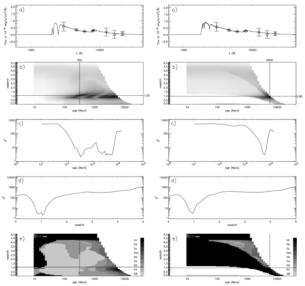
Figure 6: Fit of galaxy 319 (number from FSLY ). On the left hand side, the fit is made with model Z-PEG.2 (without age constraint) and on the right hand side we use model Z-PEG.1 (with age constraint): a) observed colors with ten times magnified error bars (for plotting only) and best-fitting synthetic SED, b) $\chi^{2}$ map on the age-$z$ plane (black corresponds to low $\chi^{2}$), c) $\chi^{2}$ projection on the age axis, d) $\chi^{2}$ projection on the redshift axis, and e) Type maps on the age-$z$ plane; the age-$z$ solutions found in b) are also plotted. The model Z-PEG.2 (left) shows several minimum redshifts around $1$ whereas model Z-PEG.1 (right) only shows one minimum close to the spectroscopic redshift ($z_{\textrm{spe}}=0.961$).

4.2 Effect of the $\Delta\lambda$  wavelength coverage

Since the strong discontinuities (4000Å, Lyman break) are the most constraining features for redshift determinations, several consequences are implied (see also discussions in Bolzonella et al. (2000) and Massarotti et al. (2001a)). The observations of colors in the near infrared is the only way to follow the discontinuities at the highest redshifts ($\leq 4.5$ for the 4000Å discontinuity and $\leq 23$ for the Lyman break in the K band). Moreover SED continua also contribute to the best fits, so that in most cases, minimizing the $\chi^{2}$ on the largest wavelength coverage will decrease the degeneracy. Figure 7 and table 2 show that without J, H and K bands, the photometric redshift determination is poor ($\sigma_{z}=0.32>\sigma_{z}=0.12$ for $z_{\textrm{\tiny spe}}<1.5$). Moreover, we do not use any filter between $8500$ and $12000$ Å to fit the data, because on the one hand we do not have the corresponding observations and on the other hand only very few galaxies in our sample are at $1<z<2$. To analyze galaxies in the redshift range $1<z<2$ , a $Z$ filter (or equivalent) would be necessary for observations as well as modeling.

Figure 7: Comparison of the photometric redshifts from Z-PEG (model Z-PEG.4) with the HDF-N measured spectroscopic redshifts without J, H, K bands, and without any particular age constraint. These results have to be compared to Fig. 5 for which there is no age constraint either. The dotted line is the linear regression of our photometric redshifts if we exclude the points with $|z_{\textrm{\tiny ZPEG}}-z_{\textrm{\tiny spe}}|\geq 1$.

4.3 IGM absorption

When comparing results with and without IGM absorption (Fig. 5), an important deviation to the spectroscopic redshifts is observed at high redshifts if we do not take the IGM into account: a linear regression on fits without the IGM shows a systematic deviation towards high photometric redshifts. This was already noted by Massarotti et al.(2001a,2001b), and can be understood quite easily: not including IGM absorption in models, one can mistake the Lyman forest absorption by intergalactic H i (below $\lambda=1216$Å) for the real Lyman break ($\lambda=912$Å in the rest frame). In such a case, we overestimate the redshift.

5 Investigations on redshifts of formation

Given the photometric redshift and age found with Z-PEG for any observed galaxy, a corresponding formation redshift $z_{for}$ , defined as the epoch of the first star’s appearance, may be derived. The result, constrained by the age of the universe (age${}_{\textrm{\tiny U}}$), depends on cosmology; as previously mentioned, standard cosmological parameters are hereafter adopted. Figure 8 shows iso-$z_{for}$ curves. The galaxy sample is also plotted and compared to curves.
For $z_{\textrm{\tiny for}}<5$, our formation redshift determination is reliable, if we keep in mind that we constrained the ages of galaxies and thus the formation redshift. Unfortunately, the precision of redshift determination from photometry is quite poor (about $0.1$ for $z<1.5$ with our sample). Above $z_{\textrm{\tiny for}}=5$, the iso-$z_{\textrm{\tiny for}}$ lines are so close to each other that we cannot rely on this formation redshift determination.
The histogram of the formation redshifts is shown in Fig. 9. Note that this histogram is in agreement with Lanzetta et al. (2001) figures of the star formation rate as a function of redshift, deduced from FSLY ’s photometry, and taking into account the effects of cosmological surface brightness.

Figure 8: Galaxies of the HDF-N sample in the redshift–age diagram, after Z-PEG fits. The dotted lines show the $z$-age relations for various $z_{\textrm{\tiny for}}$ (iso-$z_{\textrm{\tiny for}}$ lines) and the standard cosmology, previously defined. For example, the dotted line crossing the y-axis (age=0) at $z=2$ corresponds to $z_{\textrm{\tiny for}}=2$. The solid line shows the age of the universe at a given redshift (formally, this line is equivalent to $z_{\textrm{\tiny for}}=\infty$). As a result, most galaxies form at $z>3$ (we can also check this result in Fig. 9).

Figure 9: Histogram of $z_{\textrm{\tiny for}}$ from our sample. For $z_{\textrm{\tiny for}}>5$, due to the lack of precision on the determination of (age, z_phot), we cannot conclude on $z_{\textrm{\tiny for}}$ real values. $z_{\textrm{\tiny for}}=5$ is then a lower value.

6 Discussion

The determination of photometric redshifts significantly depends on the adopted evolution scenarios. The basic principle is that distant galaxies evolve according to the same basic principles as our nearby galaxies, only observed at earlier epochs. As a direct consequence, evolution scenarios must reproduce the SEDs of galaxy templates observed at $z=0$. This constraint requires meaningful statistical templates. The literature appears poor in this domain. From a large series of catalogs, we built statistical samples corrected for various effects: aperture, inclination, reddening, etc (see Fioc & Rocca-Volmerange (1999b)) in order to focus specifically on visible to near-infrared colors of eight spectral types of galaxies. All our redshifted templates are compatible with these statistical colors at $z=0$.

The evolution principles are linked to the time-dependent star formation rates. Corresponding to so-called ”monolithic” scenarios, each type evolves with a star formation rate proportional to the gas content and typical astration rates. The time-scale of star formation increases from ellipticals (half Gyr) to Irregulars (more than 10 Gyr). A test of the reliability of the adopted scenarios is given with the interpretation of the deepest multi-spectral faint galaxy counts on the largest multi-spectral coverage. Figure 5 of Fioc & Rocca-Volmerange (1999a) shows the best simultaneous fits of the deepest surveys, including the HDF-N sample, from the far-UV to the K band. The most constraining data are the reddest and deepest counts, only fitted by scenarios of old elliptical galaxy models. The evolution scenarios are from PÉGASE and similar to those used in the code Z-PEG. These considerations make the $z_{\textrm{\tiny ZPEG}}$ results more robust and the evolution scenarios of elliptical galaxies compatible with a rapid evolution at the earliest epochs. The high values of $z_{for}$ found from the present analysis favor this result. The star formation rate continuously follows the gas density, so that the current SFR depends on the past star formation history. An interesting interpretation, though tentative given the small incomplete samples, would arise if the apparent continuous law is considered as the envelop of small bursts. The intensity of these bursts decreases over time, as the gas is depleted by star formation.

If the photometric redshifts $z_{\textrm{\tiny ZPEG}}$ are faintly dependent on the adopted cosmology, the results of $z_{for}$  are more sensitive to the choice of the cosmological parameters through the age-redshift relation.

Finally the discussion of the dispersion and the degeneracy of solutions has been detailed at each step of the $z_{\textrm{\tiny phot}}$  determination. In this analysis, like the age constraint, the extension of the wavelength coverage, increasing with the number of filters, limits the degeneracy. Conversely, if galaxies are observed through only a few filters, the degeneracy may be high and results have to be used with caution.

7 Conclusions

A new code Z-PEG is proposed for public use, available on the web, to predict photometric redshifts from a data set of classical broad-band colors or spectra. The code is derived from the model PÉGASE, also available on the same web site, frequently downloaded for evolution spectrophotometric analyses and quoted in many articles. The particularity of the analysis presented here is to underline the hypotheses implicitly (or explicitly) accepted when computing photometric redshifts with evolution. The comparison with a spectrophotometric redshift sample makes the predictions robust. In its recent version PÉGASE.2, the model constrains typical evolution scenarios to fit nearby galaxies. Type-dependent extinction, IMF and metal effects are taken into account, although we assumed their modeling is not essential in our conclusions. The most constraining parameter is the $z=0$ galaxy age, typical of the nearby stellar population of each spectral type. This constraint makes it possible to eliminate implausible secondary solutions, the degeneracy being the largest cause of uncertainties on photometric redshifts. The dispersion for $z<1.5$ reaches its minimum value $0.0980$ with the age constraint, compared to other dispersion values whatever the other parameter values (IGM absorption or NIR colors). The improvement in photometric redshift accuracy brought by near-infrared colors is also measured by comparing models Z-PEG.4 and Z-PEG.2. The dispersion decreases from $0.32$ to $0.12$ for $z<1.5$ and is more important for high redshifts when the 4000Å discontinuity enters in the NIR domain and the Lyman break does not yet reach the ultraviolet bands. Finally Z-PEG is proposed to the community with PÉGASE.2. The site will be updated and improved, so that Z-PEG will also follow improvements in the spectrophotometric evolution modeling, in particular with the series of flux-calibrated samples allowing better fits of highly redshifted templates. A possible extension of Z-PEG will involve the adaptation of any photometric system, including narrow bands around emission lines, with the help of the coupled code PÉGASE+CLOUDY (Ferland (1996)), predicting stellar and photoionised gas emissions (Moy et al. (2001)).