Dynamic Hydrogen Ionization

Abstract

We investigate the ionization of hydrogen in a dynamic Solar atmosphere. The simulations include a detailed non-LTE treatment of hydrogen, calcium and helium but lack other important elements. Furthermore, the omission of magnetic fields and the one-dimensional approach make the modeling unrealistic in the upper chromosphere and higher. We discuss these limitations and show that the main results remain valid for any reasonable chromospheric conditions. As in the static case we find that the ionization of hydrogen in the chromosphere is dominated by collisional excitation in the Lyman-$\alpha$ transition followed by photoionization by Balmer continuum photons — the Lyman continuum does not play any significant role. In the transition region, collisional ionization from the ground state becomes the primary process. We show that the time scale for ionization/recombination can be estimated from the eigenvalues of a modified rate matrix where the optically thick Lyman transitions that are in detailed balance have been excluded. We find that the time scale for ionization/recombination is dominated by the slow collisional leakage from the ground state to the first excited state. Throughout the chromosphere the time scale is long ($10^{3}$-$10^{5}$ s), except in shocks where the increased temperature and density shorten the time scale for ionization/recombination, especially in the upper chromosphere. Because the relaxation time scale is much longer than dynamic time scales, hydrogen ionization does not have time to reach its equilibrium value and its fluctuations are much smaller than the variation of its statistical equilibrium value appropriate for the instantaneous conditions. Because the ionization and recombination rates increase with increasing temperature and density, ionization in shocks is more rapid than recombination behind them. Therefore, the ionization state tends to represent the higher temperature of the shocks, and the mean electron density is up to a factor of six higher than the electron density calculated in statistical equilibrium from the mean atmosphere. The simulations show that a static picture and a dynamic picture of the chromosphere are fundamentally different and that time variations are crucial for our understanding of the chromosphere itself and the spectral features formed there.

1 Introduction

The solar chromosphere is the region about 1.5 Mm thick between the temperature minimum (at about 4000 K) and the transition region to coronal temperatures of several million Kelvin. Traditionally, its structure has been determined by semi-empirical fitting of temporally and spatially averaged continua and line intensities (e.g., Vernazza et al., 1981; Maltby et al., 1986; Fontenla et al., 1993). However, the chromosphere is actually a very dynamic region. In this paper we investigate the hydrogen ionization structure of a dynamic chromosphere.

It has long been known that hydrogen ionization and excitation in the solar atmosphere is not in equilibrium for the local temperature and density (Thomas, 1948). Usually, hydrogen ionization is calculated from the condition of “statistical equilibrium”, that is, the equality of the ionization and recombination rates for the local temperature, density and radiation. Statistical equilibrium assumes infinitely fast rates and an instantaneous adjustment to the local thermodynamic and radiation state. However, if the local state changes in time, or if there is a flow through a inhomogeneous region, and if the time scale to reach ionization or excitation equilibrium is longer than the dynamic times scale, then it is necessary to solve the population rate equations,

$${{dn_{i}}\over{dt}}={\rm gains-losses}\ ,$$

for each species $i$ (Joselyn et al., 1979). This latter is the case in the solar atmosphere heated by any intermittent process (such as shocks or nanoflares) (Elzner, 1975; Klein et al., 1976; Kneer & Nakagawa, 1976; Poletto, 1979; Kneer, 1980). The ionization and excitation state then depends on its history as well as the instantaneous temperature, density and radiation. However, the importance of slow chemical reaction rates in the quiet solar atmosphere has generally been neglected since these early papers were written. The active solar atmosphere (e.g. flares, prominence formation and coronal mass ejections) has long been recognized to require a time dependent analysis (McClymont & Canfield, 1983; Doschek, 1984; Fisher et al., 1985; Heinzel, 1991; Abbett & Hawley, 1999; Sarro et al., 1999; Ciaravella et al., 2001; Ding et al., 2001; Lanza et al., 2001). The same issue of ionization and other chemical reaction rates being slow compared to the rate of dynamical changes, and thus requiring the solution of the species rate equations rather than statistical equilibrium, arises in many other areas of astrophysics where conditions are changing in time. Examples are: the interstellar medium (Lyu & Bruhweiler, 1996; Joulain et al., 1998), HII regions (Rodriguez-Gaspar & Tenorio-Tagle, 1998; Richling & Yorke, 2000), planetary nebula (Schmidt-Voigt & Koeppen, 1987; Frank & Mellema, 1994; Marten & Szczerba, 1997), novae (Hauschildt et al., 1992; Beck et al., 1995), supernova (Kozma & Fransson, 1998), and the reionization of the intergalactic medium and the Ly_α forest (Ikeuchi & Ostriker, 1986; Shapiro & Kang, 1987; Shapiro et al., 1994; Ferrara & Giallongo, 1996; Giroux & Shapiro, 1996; Zhang et al., 1997).

The solar chromosphere is not well represented by a static mean structure. We show that because the chromosphere is dynamic the average hydrogen ionization is significantly different from the ionization state of the mean atmosphere. There are two reasons for this. First, the mean of any quantity that depends non-linearly on the atmospheric properties is not the same as that quantity determined from the mean atmosphere. Second, the finite rates of ionization and recombination reduce the response of the ionization to dynamic variations in the atmospheric state. Hydrogen does not have time to reach its equilibrium ionization. The result is a hydrogen ionization fraction that is higher than obtained for the mean of the dynamic atmosphere. This conclusion is independent of just what that mean state is. Thus analyzing observations on the basis of a static model chromosphere leads to very different conclusions from an analysis based on a dynamic model chromosphere. This significantly alters the interpretation of observations.

In this paper, we first describe (section 2) the numerical simulations used to study the dynamic hydrogen ionization. We then show that the dominant hydrogen ionization process is photoionization from the second level and we investigate the processes that populate the second level (section 3). There is a very rapid equilibration of the 2^nd and all higher levels with the continuum, with a slow collisional leakage of electrons from the ground state to the 2^nd level, or visa versa, depending on whether hydrogen is ionizing or recombining. Next we calculate the time scale for ionization/recombination and its relation to the eigenvalues of the rate matrix (section 4). The ionization and recombination rates are slow and not in equilibrium, so that the level populations change in time. We demonstrate that there is only one relaxation time scale to approach equilibrium, not separate ionization and recombination times scales. We show (section 5) that because of the slow ionization and recombination rates, the dynamic ionization fluctuates much less than the statistical equilibrium ionization. As a result, line and continuum intensity variations do not mimic the underlying dynamics. Further, the mean ionization fraction tends to represent the maximum statistical equilibrium ionization, and is much higher than is obtained from the statistical equilibrium of the mean atmosphere. We conclude (section 6) with a reiteration of why the chromosphere must be dynamic based on fundamental physical principles and observations and a statement of which results are robust and why.

2 Numerical Simulations

To properly model the dynamic solar chromosphere one has to perform radiation-hydrodynamic simulations taking into account the non-local, non-linear rate equations for all important species. Such a self-consistent radiation-hydrodynamic modeling of the solar chromosphere has been performed by Carlsson & Stein (1992, 1994, 1995, 1997a, 1997b) and we summarize the methodology here.

We solve the one-dimensional equations of mass, momentum, energy and charge conservation together with the non-LTE radiative transfer and population rate equations, implicitly on an adaptive mesh. Advection is treated using Van Leer’s (1977) second order upwind scheme to ensure stability and monotonicity in the presence of shocks. An adaptive mesh is used (Dorfi & Drury, 1987) in order to resolve the regions where the atomic level populations are changing rapidly (such as in shocks). The equations are solved simultaneously and implicitly to ensure self-consistency and stability in the presence of radiative energy transfer, stiff population rate equations, and to have the time steps controlled by the rate of change of the variables and not by the small Courant time for the smallest zones. A linearization method is used to solve the radiative transfer (Scharmer & Carlsson, 1985) but with a penta-diagonal approximate lambda operator (Rybicki & Hummer, 1991) instead of the global Scharmer operator. The effects of non-equilibrium ionization, excitation, and radiative energy exchange from several atomic species (H, He and Ca) on fluid motions and the effect of motion on the emitted radiation from these species are calculated. We model hydrogen and singly ionized calcium by 6 level atoms and helium with a 9 level atom. For helium we collapse terms to collective levels and include the $1s^{2}$, $2s$ and $2p$ terms in the singlet system and the $2s$ and $2p$ terms in the triplet system of neutral helium, and the $1s$, $2s$ and $2p$ terms of singly ionized helium. In addition we include doubly ionized helium. We include in detail all transitions between these levels. For singly ionized calcium they are the H and K resonance lines, the infrared triplet and the photoionization continua from the five lowest levels. We use 31–101 frequency points in each line and 4–23 frequency points in each continuum; a total of 1424 frequency points. Continua from elements other than H, He and Ca are treated as background continua in LTE, using the Uppsala atmospheres program (Gustafsson, 1973).

The upper boundary is a corona at 10⁶K with a transmitting boundary condition. Incident radiation from the corona is included which causes ionization in the helium continua in the upper chromosphere. The lower boundary condition, at 500 km below $\tau_{500}\!=\!1$, is also transmitting. Waves are driven through the atmosphere by a piston located at the bottom of the computational domain. The piston velocity is chosen to reproduce a 3750 second sequence of Doppler-shift observations in an Fe I line at $\lambda$396.68 nm in the wing of the Ca H-line (Lites, Rutten & Kalkofen 1993) This line is formed about 260 km above $\tau_{500}\!=\!1$.

The initial atmosphere (Fig. 1) is in radiative equilibrium above the convection zone (for the processes we consider) without line blanketing and extends 500 km into the convection zone, with a time constant divergence of the convective energy flux (on a column mass scale) calculated with the Uppsala code without line blanketing. Note that the transition region in the initial atmosphere occurs at a lower height than in standard models. This is because the lower temperature means a smaller pressure scale height and a less extended atmosphere. The atmospheric dynamics moves it outwards on average. The transition region occurs at a smaller pressure than in the VALIIIC model. This is set by the amount of conductive flux at the upper boundary and is a free parameter in the model (follows from the location of the upper boundary at the fixed temperature of 10⁶K). The mean structure of the dynamic atmosphere (Fig. 1) has a low (5000 K) temperature throughout most of the chromosphere, with a temperature rise in the upper chromosphere produced by absorption of coronal radiation in the helium continua.

Figure 1: Initial and mean state of the atmosphere. Temperature (solid lines) and electron density (dashed lines) as functions of column mass. The initial state is shown with thin lines and the mean of the second half of the simulation is shown with thick lines. The height scale is that of the initial atmosphere. The mean temperature is close to the initial radiative equilibrium state while the mean electron density is up to a factor six larger than the initial value. For comparison, the temperature and electron density as functions of column mass of the VALIIIC model are shown with dotted lines.

The difference between the calculations reported here and the ones in the references cited above is that we now include helium, a corona and transition region, the incident radiation from the corona, extend the calculations deeper and have a transmitting lower boundary condition. This makes it possible to discuss the upper chromosphere, in particular the ionization of hydrogen, in some more detail than before.

The validity of these simulations can be checked by comparing their predictions with observations. There is both agreement with some observations and disagreement with other observations. CO molecular line observations indicate that there is no temperature rise in the low chromosphere, consistent with the simulation. The simulations reproduce many details in observations of the calcium H-line (Carlsson & Stein, 1997a). The Ca grains are due to waves that steepen into shocks around a height of 1 Mm. However, the cores of the simulated H and K lines are darker and the bright points are brighter than is observed. The Lyman continuum intensity variation is also larger in the simulations than what is observed. There is a possible disagreement with SUMER observations that the cores of NI, OI, CI and CII lines, formed in the mid and upper chromosphere, show emission everywhere. Although some of these line cores are formed below the height where coronal radiative heating raises the mean chromospheric temperature, there is some contribution from that region of enhanced temperature. Preliminary calculations (that are non-trivial because effects of slow ionization/recombination have to be included, as is shown in this paper) show that this contribution actually cause the lines to be in emission all the time even though the average line emission is weaker than is observed.

The improved physics in the simulations reported on here compared with the previous work (the inclusion of a corona and the absorption of coronal radiation in the helium continua) has improved the agreement; the line cores in the calcium H and K lines are not as dark as in the previous simulations, the rms variation in the Lyman continuum radiation temperature has changed from 256 K (Carlsson & Stein 1994, 1997b) to 97 K (compared to an observed value of about 40 K) and UV lines from neutral elements now seem to be in emission everywhere in the simulations.

The existing disagreements indicate that there is still physics missing from the simulations. For instance, we do not include line blanketing (especially the numerous iron lines), the CO molecule and the singly ionized magnesium atom (producing the Mg h and k lines). We use a crude approximation to partial redistribution of radiation in the Lyman lines and no partial redistribution at all in the calcium H and K lines. We do not include frequencies above 20 mHz in the driving piston. We do not include the effects of magnetic fields.

Assuming complete redistribution in the calcium lines probably leads to an overestimate of the cooling in these lines by up to a factor of two (Uitenbroek, 2002), partially compensating the omission of the magnesium h and k lines. High frequency waves may lead to heating of the mid chromosphere through dissipation in shocks and the neglect of high frequencies in the driving piston probably leads to a lower mean temperature.

Magnetic fields structure the chromosphere and corona (Aschwanden et al., 2001; Berger et al., 1999; Schrijver et al., 1999; Moses et al., 1994). They influence both energy transport (wave modes and quasi-static driving) and heating (nanoflares, resonant wave absorption). In the photosphere magnetic fields are concentrated into isolated flux tubes or loops, except in very high magnetic flux regions, leaving most of the photosphere nearly field free. The upper convection zone is the site of acoustic wave generation (Stein & Nordlund, 2001; Skartlien et al., 2000; Goldreich et al., 1994), while overshooting convective flows in the photosphere generate gravity waves. MHD tube waves are driven by convective motions acting on the localized magnetic fields (Musielak & Ulmschneider, 2001). The photospheric tubes and loops spread out with increasing height and decreasing gas pressure. When acoustic waves propagate into the the region where the magnetic pressure equals the gas pressure ($\beta=1$) and the magnetic field lines are curved, there is significant reflection and mode conversion into magneto-hydrodynamic waves propagating at approximately the Alfven speed (Rosenthal et al., 2002). These latter are less compressive and have a smaller amplitude for a given flux than the acoustic waves, because of their faster propagation speed, and hence are less visible. Where there is magnetic field extra heating occurs — continuum intensities and line emissions are substantially higher in magnetic network regions than in the internetwork. It is likely that the same processes will contribute to the heating in internetwork regions in the mid-chromosphere where the magnetic field spreads to form a ”magnetic canopy”.

In this paper we focus on the processes controlling the ionization of hydrogen in a dynamic atmosphere. We show that when chemical rates are slow, populations do not have time to reach their equilibrium values. Indeed, some of the disagreement with observations may be due to this non-equilibrium. The solar chromosphere will experience some additional heating besides that included in our model. However, as we show later, even in such hotter models the ionization/recombination rates are slow and the results presented here will be qualitatively correct.

3 Ionization and Excitation Processes

In the upper chromosphere and lower transition region the density is much too low to ensure LTE and the full rate equations have to be solved to calculate the hydrogen ionization. Furthermore, inspection of the rates involved shows that typical ionization/recombination time scales are much longer than dynamical time scales so that the ionization balance can be expected to be out of statistical equilibrium. It is thus necessary to take into account the advection and time-derivative terms in the equations. In this section we analyze the rate equations to find what processes dominate the hydrogen ionization balance. In the next section we analyze the time scales involved.

Figure 2 shows the hydrogen ionization fraction as a function of column mass ($m_{c}$) in the initial radiative equilibrium atmosphere. The ionization fraction rises from about $10^{-5}$ at the classical temperature minimum at lg($m_{c}$)=$-1$ (height of 0.5 Mm) to about 30% at the base of the transition region 1 Mm further up.

Figure 2: Hydrogen ionization as a function of column mass in the initial radiative equilibrium atmosphere.The ionization fraction rises from about $10^{-5}$ at the classical temperature minimum at lg($m_{c}$)=$-1$ (height of 0.5 Mm) to about 30% at the base of the transition region 1 Mm further up.

The processes that are important for the ionization balance are not the same in the transition region and in the chromosphere. In the solar chromosphere the hydrogen ionization is dominated by photoionization from the first excited state. The reason is that the much lower particle density of the first excited state ($\approx 3\times 10^{4}{\rm cm}^{-3}$) than in the ground state ($\approx 10^{11}{\rm cm}^{-3}$) is more than compensated by the higher mean intensity at the Balmer edge at 364 nm compared to that of the Lyman edge at 91 nm. At a radiation temperature of 5000 K the ratio is $3\times 10^{8}$. In addition, the atmosphere is optically thick to Lyman photons and optically thin to Balmer photons in all of the chromosphere. The result is that photoionization by Lyman photons plays an insignificant role in the hydrogen ionization throughout the chromosphere. Figure 3 shows the net rates between all the hydrogen energy levels at lg($m_{c}$)=$-4$ which corresponds to a height of 1.2 Mm in the initial atmosphere. This picture is almost identical in the whole chromosphere from lg($m_{c}$)=$-1$ up to the base of the transition region at lg($m_{c}$)=$-5.6$. Ionization is primarily through a net rate from $n$=2 to the continuum (photoionization in the Balmer continuum) balanced by recombination to the higher levels cascading down to the $n$=2 level through bound-bound transitions with $\Delta n$=1. The reservoir of electrons is the ground state. There is transfer of electrons between the ground state and first excited state by collisions. The rate of this transfer is very slow, because chromospheric temperatures are of order 1 eV and the energy jump to the first excited level is 10.2 eV.

In the very thin zone (2 km) where the ionization fraction goes from 30% to fully ionized the situation is different. Collisional ionization from the ground state dominates with net photorecombination in all continua and again bound-bound transitions with $\Delta n$=1 dominating the return channel to the ground state (Fig. 4).

Figure 3: Net rates between the hydrogen levels in the chromosphere (at lg($m_{c}$)=$-4$ which corresponds to a height of 1.2 Mm in the initial atmosphere, but the picture is almost identical in the whole chromosphere from lg($m_{c}$)=$-1$ up to the base of the transition region at lg($m_{c}$)=$-5.6$). The thickness is proportional to the net rate with arrows showing the direction of the net rate. The ionization is dominated by photoionization in the Balmer continuum balanced by photorecombination to higher levels and cascades through bound-bound transitions with $\Delta n$=1.

Figure 4: Same as Fig. 3 but for a point in the transition region where T=20000K. The ionization is dominated by collisional ionization from the ground state balanced by photorecombination to all levels.

Figures 3-4 only show the net rates and do not answer the question what is driving the system and what rates are just adjusting to provide a closed loop. One way to investigate this aspect is to see how the system responds to perturbations. We have therefore solved the equations of statistical equilibrium repeatedly perturbing the rates one-by-one. Increasing the photoionization cross-section in the Balmer continuum increases the ionization while the opposite is true for the bound-free transitions from the higher levels, consistent with the rate picture where the ionization is through photoionization in the Balmer continuum and recombination to the higher levels. Even though the H-$\alpha$ ($n$=3 $\rightarrow$ $n$=2) transition has the largest net rate in the chromosphere changing this rate has no effect on the ionization balance. The same is true for all other bound-bound transitions except for Ly${\alpha}$. Increasing the Ly${\alpha}$ rate increases the ionization slightly just below the transition region where absorption in Ly${\alpha}$ of photons from the transition region and corona populates level 2.

Figure 5: The temperature (left column, dashed line, right axis) and hydrogen ionization fraction (left column, solid line, left axis) together with the rates (right column) as a function of column mass and time in a simulation of the solar chromosphere and lower transition region. Rates are given from the bound levels $n$=1-5 to the continuum with no symbols on radiative rates and diamonds added for collisional rates. Positive rates indicate ionization, negative rates recombination. Before the shock forms the rates are in equilibrium (plus signs close to zero) dominated by photoionization in the Balmer continuum and recombination to the higher levels (top right panel). As the shock progresses upwards the rates become larger and Balmer photoionization dominates without a balancing recombination to the highly excited levels. Direct ionization from the ground state is always small below the transition region.

Up to now we have studied only the static atmosphere. Hydrogen ionization in a dynamic chromosphere is illustrated in Fig. 5. In the left column the temperature is shown as a function of column mass as a dashed line with the values shown on the right hand axes. The same column shows the hydrogen ionization fraction on a logarithmic scale as a solid line with values on the left axes. The right column shows the net rates from the bound hydrogen levels $n$=1-5 to the continuum with positive values indicating net ionization, negative values recombination. Time progresses from the top panel downwards.

At a time 1600 seconds from the start of the simulation a shock is starting to form around lg($m_{c}$)= $-3.5$ (height of 1 Mm). The rates are in statistical equilibrium (the sum of the rates is close to zero) with a balance between Balmer photoionization and recombination to the levels $n$=2-5. 20 seconds later (mid panels) the shock has formed. Balmer photoionization is greatly increased in the shock, because the population of the first excited state has greatly increased due to collisional excitation from the ground state . (The ratio of collisional excitation to de-excitation rates depends exponentially on temperature, $C_{12}/C_{21}=g_{2}/g_{1}e^{-\Delta E/kT}$.) The Ly${\alpha}$ transition is found to be in detailed balance and so just bounces electrons up and down. The photoionization rate per atom is constant because it depends on the radiation field which is set deeper down in the atmosphere. Balmer photoionization dominates the rates into the continuum (dotted curve), but it is not balanced by recombination (because of slow rates) resulting in a net increase of protons (sum of rates positive and almost equal to the Balmer photoionization). As the shock progresses farther upwards, recombination dominates over photoionization behind the shock. The zone where hydrogen goes from 1% to 40% ionization is about 600 km thick.

At the top of the chromosphere hydrogen is between 30 and 40% ionized. The further ionization up to 100% ionization takes place in the zone where the temperature increases from 10000 K to 25000 K. The ionization rates are here dominated by collisional ionization directly from the ground-state while the Lyman continuum actually provides some net recombination. The thickness of this zone depends on the temperature gradient and is thus very model dependent — in the plane parallel calculations this zone is very thin, on the order of 2 km. Also in this zone we see rates that are out of statistical equilibrium with net ionization when shocks pass followed by net recombination.

4 Time Scales

The crucial result of our investigation is that the time scale for changes in the ionization of hydrogen in the chromosphere is long, because the rates for ionization and recombination under conditions typical of the solar chromosphere are small. Consequently the hydrogen populations do not adjust to the local conditions.

The relation of time scales and transition rates can be understood most readily for the case of a 2-level atom. We summarize the well known results here. The equations for the populations of levels 1 and 2 are

$${{Dn_{1}}\over{Dt}} = n_{2}P_{21}-n_{1}P_{12}$$ (1)

$$n_{1}+n_{2} = n_{H}\ ,$$ (2)

where $n_{i}$ is the population of level $i$ and $P_{ij}$ is the transition rate per atom (radiative $R_{ij}$ plus collisional $C_{ij}$) from level $i$ to level $j$, and $n_{H}$ is the total hydrogen number density. The solution for the population of level $1$ is

$$n_{1}(t)=n_{1}(\infty)+\left(n_{1}(0)-n_{1}(\infty)\right)e^{-t(P_{21}+P_{12})}\ ,$$ (3)

where $n_{1}(\infty)$ is the equilibrium population achieved at infinite time,

$$n_{1}(\infty)={{n_{H}P_{21}}\over{P_{21}+P_{12}}}\ .$$ (4)

Thus there is only one time scale for for the approach to ionization equilibrium

$$\tau_{relax}=1/\left(P_{21}+P_{12}\right)\ .$$ (5)

It is wrong to talk about separate time scales, one for ionization and one for recombination, even though there are distinct ionization and recombination rates. Also, this result of an exponential approach to a final equilibrium state with a given time scale assumes that the ionization and recombination rates per atom are constant in time. In the real case where the rates per atom are themselves evolving (because of changes in the radiation field and electron density) the concept of a time scale is not well defined, although it is still useful.

When the rate of upward radiative transitions balances the rate of downward radiative transitions, $n_{1}R_{12}=n_{2}R_{21}$, the equations can be simplified by assuming that this holds exactly, which is called detailed balance. In this case, $n_{i}P_{ij}\rightarrow n_{i}C_{ij}$ and the solution for the population of level one is

$$n_{1}(t)=n_{1}(\infty)+\left(n_{1}(0)-n_{1}(\infty)\right)e^{-t(C_{21}+C_{12})}\ ,$$ (6)

where now the final equilibrium population is

$$n_{1}(\infty)={{n_{H}C_{21}}\over{C_{21}+C_{12}}}\ ,$$ (7)

and the relaxation time scale is

$$\tau_{relax}=1/\left(C_{21}+C_{12}\right)\ .$$ (8)

This assumption of detail balance thus implies that the radiative rates per atom change with time as the populations relax to their equilibrium state, so that

$${{R_{12}}\over{R_{21}}}={{n_{2}}\over{n_{1}}}={{n_{2}(\infty)-\left(n_{1}(0)-n_{1}(\infty)\right)e^{-t(C_{21}+C_{12})}}\over{{n_{1}(\infty)+\left(n_{1}(0)-n_{1}(\infty)\right)e^{-t(C_{21}+C_{12})}}}}\ .$$ (9)

Another possible simplification is to express the radiative rates in terms of the net radiative bracket (NRB),

$$n_{2}R_{21}-n_{1}R_{12}=n_{2}R_{21}\left(1-{{n_{1}}\over{n_{2}}}{{R_{12}\over{R_{21}}}}\right)=n_{2}R_{21}\cdot{NRB}\ .$$ (10)

In this case the equation for the level 1 population becomes

$${{Dn_{1}}\over{Dt}}=n_{2}\left(C_{21}+R_{21}\cdot{NRB}\right)-n_{1}C_{12}\ .$$ (11)

If it is assumed that both the rates per atom and the NRB are constant, then the solution for the population is

$$n_{1}(t)=n_{1}(\infty)+\left(n_{1}(0)-n_{1}(\infty)\right)e^{-t(C_{21}+C_{12}+R_{21}\cdot{NRB})}\ ,$$ (12)

where now the final equilibrium population is

$$n_{1}(\infty)=n_{H}{{C_{21}+R_{21}\cdot NRB}\over{C_{21}+C_{12}+R_{21}\cdot NRB}}\ ,$$ (13)

and the time scale to approach equilibrium is

$$\tau_{relax}=1/\left(C_{21}+C_{12}+R_{21}\cdot{NRB}\right)\ .$$ (14)

If the net radiative transition rate is small compared to the upward and downward rates individually, then the NRB will be very small, so the radiative rates will make only a small change in the relaxation time scale given by the collisional rates. The radiative transitions can either increase (if NRB $<$ 0) or decrease (if NRB $>$ 0) the relaxation time scale.

We have calculated the relaxation time scale (at each height and each time step) from our numerical simulation. We proceeded in the following way: The value of the hydrodynamic variables were taken from a given time step and kept constant in time for the relaxation time scale calculation. The population densities consistent with this state of the atmosphere were calculated by solving the equations of statistical equilibrium. This defined the initial population density in the ionized state, $n_{p}(0)$. This atmosphere was then perturbed by increasing the temperature by 1% throughout. The populations consistent with this perturbed state was calculated from the equations of statistical equilibrium giving the asymptotic solution, $n_{p}(\infty)$. The time evolution from the initial state of the number of protons at a given height was also calculated using the full rate equations, defining $n_{p}(t)$. The numerical solution was cast in a 2-level form (see above) and the relaxation time scale was calculated from a least-squares linear fit to

$$\ln\left[{{n_{p}(t)-n_{p}(\infty)}\over{n_{p}(0)-n_{p}(\infty)}}\right]=-{t\over\tau_{relax}}\ .$$ (15)

The relaxation time scale for hydrogen ionization/recombination, as found from the numerical simulation, from the photosphere to the transition region, is shown in Fig. 6 (thick solid line). The time scale increases outward from the $\sim 1$ sec. in the photosphere to $\sim 10^{5}$ sec in the mid chromosphere and then decreases to $\sim 10^{2}$ sec. at the base of the transition region.

Figure 6: Relaxation time scale as function of column mass. The numerically determined relaxation time scale is given as the thick solid line. Time scales determined from eigenvalues of the rate matrix are also shown for several cases: full rate matrix (dotted), collisions only (dot-dashed), Lyman transitions in detailed balance (thin solid) and Ly$\alpha$ treated with a constant net radiative bracket (dashed). The electron density is given as the thick dashed curve. The ionization/recombination time scale becomes very long in the chromosphere. Eigenvalues calculated from a rate matrix with all the radiative and collisional rates give a time scale several orders of magnitude too short. Eigenvalues calculated from a rate matrix with all Lyman radiative transitions in detailed balance except for Ly$\alpha$, which is included using its net radiative bracket, give a time scale that closely matches the numerical result.

The eigenvalues and eigenvectors of the rate matrix, $P_{ij}$ with $P_{ii}=\sum_{j}P_{ij}$ (where $P_{ij}$ is the transition rate per atom from level $i$ to level $j$), help to clarify the processes controlling the time scale. The relaxation process can be represented by the equation

$$\mathbf{n}=\sum_{i=0,5}c_{i}\mathbf{v_{i}}e^{\lambda_{i}t}\ ,$$ (16)

where $\mathbf{n}$ is the vector of the level populations,

$$\mathbf{n}=\left(\begin{array}[]{c}n_{1}\\ n_{2}\\ n_{3}\\ n_{4}\\ n_{5}\\ n_{6}\end{array}\right)\ .$$ (17)

Here level 1 is the ground state and level 6 is the continuum. $\mathbf{v_{i}}$ is the eigenvector corresponding to the $i^{th}$ eigenvalue $\lambda_{i}$. The coefficients $c_{i}$ depend on the initial conditions. There is a zero eigenvalue whose eigenvector is the equilibrium state. The other eigenvalues are all negative, since the populations are relaxing toward their equilibrium value.

The numerically determined relaxation time scale is compared with the time scale from the eigenvalue calculation, which is the inverse of the smallest (in absolute value) non-zero eigenvalue, in Fig. 6. We have calculated the eigenvalues using several different assumptions about the rate matrix. Note, first of all, that when all the processes are included in the rate matrix the time scale obtained from the eigenvalues (dotted line) is orders of magnitude smaller than found in the numerical solution (thick solid line). The time scale obtained from the rate matrix with only collisional rates (dot dash line) has the same general pattern as the numerical time scale, but is generally slightly larger. When radiative rates are added, but with all the Lyman transitions assumed to be in detailed balance, the time scale from the eigenvalues of the rate matrix (thin solid line) reproduce the numerical time scale up to the peak in the mid-chromosphere. This indicates that in this region the large Lyman radiative rates are in fact changing with time so as to maintain nearly detailed balance as the populations change. The general behavior of the relaxation time is thus controlled by the collisional processes. The time scale increases from the photosphere to the mid chromosphere, where the electron density has a minimum approximately as the inverse of the collisional recombination rate ($\propto n_{e}^{-2}$). From the mid-chromosphere to the transition region the time scale decreases, first because the electron density (thick dashed line) increases as the increasing ionization fraction of hydrogen more than offsets the outwardly decreasing overall density, and second because the temperature starts to increase due to absorption of coronal photons. The upward collisional rates are exponentially sensitive to the temperature. Radiative transitions generally reduce the time scale by a factor of about 4 from the all collision case. The wiggles in the relaxation time above its peak in the mid-chromosphere are nearly reproduced if the net Ly${\alpha}$ radiative transition is included as a constant net radiative bracket (dashed line). Where Ly${\alpha}$ photons begin to leak through the atmosphere they increase the relaxation time because in that region they produce a net increase in the population of the second level while collisions produce a net depopulation of the second level. Hence, the Ly${\alpha}$ net radiative bracket is negative and as seen in the two level case this increases the relaxation time.

The role of the various transitions in the equilibration process can be determined from the eigenvectors and eigenvalues appearing in eqn. 16. We study the level in the atmosphere at column mass density $m_{c}=10^{-4}$ in the initial atmosphere, and treat the Lyman transitions in detailed balance except for Ly${\alpha}$ which is treated via its net radiative bracket. The slowest process, with eigenvalue $-2.2\times 10^{-6}\,{\rm s}^{-1}$, has the eigenvector

$$\mathbf{v_{1}}=\left(\begin{array}[]{c}-0.7\\ 2\times 10^{-7}\\ 1\times 10^{-9}\\ 4\times 10^{-10}\\ 3\times 10^{-10}\\ 0.7\end{array}\right)\ .$$ (18)

which thus represents the relaxation between the ground state and the continuum. The next slowest process, which is 10 orders of magnitude faster, with eigenvalue $-2\times 10^{4}\,{\rm s}^{-1}$, has the eigenvector

$$\mathbf{v_{2}}=\left(\begin{array}[]{c}-2\times 10^{-4}\\ 0.7\\ 4\times 10^{-3}\\ 1\times 10^{-3}\\ 9\times 10^{-4}\\ -0.7\end{array}\right)\ .$$ (19)

and is relaxation between the second level and the continuum. The fastest relaxation processes, all with eigenvalues of order $-1\times 10^{7}\,{\rm s}^{-1}$, are between level 2 and levels 3, 4 and 5. In the chromosphere, unlike the transition region, ground state relaxation does not take place via direct level 1 $\leftrightarrow$ continuum transitions, but rather through a level 1 $\leftrightarrow$ 2 transition followed by level 2 $\leftrightarrow$ higher levels and continuum transitions (Fig. 3). Thus the process of hydrogen ionization in the chromosphere can be thought of as a very rapid (small fraction of a second) equilibration of the 2^nd and all higher levels with the continuum, together with a slow leakage of electrons from the ground state to the 2^nd level, or visa versa, depending on whether hydrogen is ionizing or recombining.

5 Consequences of Slow Rates

The ionization structure of a dynamic atmosphere is very different from that of a static atmosphere. The ionization/relaxation time scale decreases dramatically (to about 10 - $10^{3}$ sec.) in chromospheric shocks, where the temperature increases significantly and to a lesser extent in the elevated temperature tail of the shocks (Fig. 7). As a shock propagates upward it strengthens and the time scale becomes shorter. However, the time scale is still too long for the ionization to reach its equilibrium value in the shock and the peak ionization occurs behind the shock front (Fig. 7). The slow ionization results in more of the shock energy going into raising the temperature rather than ionizing the gas (Carlsson & Stein, 1992).

The primary processes controlling the ionization in shocks is the same as for the static atmosphere: photoionization from the Balmer level and photorecombination to the higher levels, with slow leakage between the ground state and the 2^nd level. The high temperature (and density) in the shocks increases the collisional and radiative leakage rates between the ground state and the 2^nd level which leads to a smaller relaxation time. Balmer photoionization has the greatest increase, both within the shock and in the post shock tail (Fig. 5). In the shock itself, the sum of all the ionization/recombination rates is approximately equal to the Balmer photoionization rate alone. That is, almost all the ionization is occurring as Balmer photoionization and there is little balancing recombination. Thus the ionization is not in statistical equilibrium and there is net ionizing in the shock. In the mid-chromosphere there is net ionization even in the post shock tail, though at a slower rate. When the shocks reach the upper chromosphere, increased recombination to the third and higher levels leads to net recombination in the post shock tail, but at a much slower rate than the initial ionization in the shock (Fig. 5, t= 1650 s). Because the time scale is short in the shock where hydrogen is ionizing, due to the high temperature, but longer in the post shock region, where the temperature decreases and hydrogen is recombining, the steady state level of hydrogen ionization tends toward the value approximating the peak ionization in the shocks (Fig. 8).

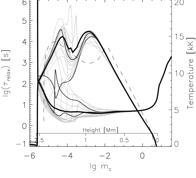
Figure 7: Relaxation time scale (upper curves, scale to the left) and temperature (lower curves, scale to the right) as function of column mass and time in the dynamic simulation. The height scale of the initial state is also given. The mean relaxation time scale and the mean temperature over the second half of the simulation are given with thick solid lines. Two particular instances are given in black with a number of other instances in grey. The time scale for ionization/recombination is much reduced in shocks where hydrogen is ionizing and also reduced, but to a lesser extent, in shock wakes where hydrogen is recombining. The relaxation time scale calculated from the VALIIIC semi-empirical model is given as function of column mass for comparison (dashed line).

In the photosphere (e.g. initial height of 0.4 Mm), the dynamical ionization fraction follows the statistical equilibrium one with a delay of 20-40 seconds and the ionization fraction is about $10^{-5}$ (Fig. 8). By the low chromosphere (initial height of 0.6 Mm) the rates become too slow to keep up with the dynamic variations of density and temperature and the ionization fraction shows much smaller variations than in equilibrium. The ionization fraction increases with time from $2\times 10^{-5}$ to a steady state value of $10^{-4}$. In the mid-chromosphere (initial height 1.0 Mm) the rates are so slow that the ionization variation does not follow the dynamics at all. There is a slow, secular increase in the steady state ionization fraction from $10^{-4}$ to $10^{-2}$. At the same values of the hydrodynamic variables the statistical equilibrium ionization varies by six orders of magnitude. The behavior slightly higher (at 1.4 Mm) is similar. The slow ionization/recombination rates thus cause the ionization fraction to vary much less than in equilibrium and the mean ionization fraction represents the conditions at the peaks of the shocks and is substantially higher than the mean equilibrium value.

Figure 8: Ionization fraction as function of time at four different Lagrangian locations (labeled with their initial height). The solid line shows the actual ionization fraction in the simulation, the dotted line shows the ionization fraction calculated from statistical equilibrium at the same values of the hydrodynamic variables. In the chromosphere, the ionization tends toward the equilibrium value appropriate for the shock peaks and its variation is small.

The small amplitude of the electron density variations compared with their equilibrium values and the fact that the mean electron density samples the peaks of the shocks rather than the mean conditions have several consequences for the proper interpretation of chromospheric diagnostics.

The intensity of collisionally excited lines will vary much less than the hydrodynamic variations would imply. An analysis based on equilibrium values of the electron density would give too low amplitudes for the atmospheric variations even if the effects of departures from LTE are taken fully into account.

Classical static models of the solar chromosphere are based on temporal and spatial averages of intensity — either continuum intensities shortward of the silicon edge at 152 nm (like in the models by Avrett and co-workers, e.g., Vernazza et al. (1981), Maltby et al. (1986), Fontenla et al. (1993)) or line profiles of resonance lines from ionized calcium and magnesium. The mean is taken in the ultraviolet part of the spectrum where the temperature dependence of the Planck function is more exponential than linear. Although the source function is quite decoupled from the Planck function and has a smaller amplitude than the local Planck function, the mean source function preferentially samples the high temperatures in shocks. This was dramatically illustrated in Carlsson & Stein (1995) where the best semi-empirical fit to the mean intensities in the simulation showed a chromospheric temperature rise while the mean temperature showed no increase.

At long wavelengths the Planck function has a linear dependency on temperature and one avoids the effect of averaging a non-linear function (at ultraviolet wavelengths) that gives an exaggerated temperature increase with height. The temporal average of the intensity at mm and sub-mm wavelengths should give the mean temperature as function of height provided the formation is in LTE. However, the electron density sampling of shock conditions at long wavelengths has a similar effect as temperature sampling of shocks at short wavelengths and an analysis based on equilibrium values will give an exaggerated temperature increase with height. The current simulations do, in fact, match observations made at long wavelengths remarkably well (Loukitcheva et al., 2001). The conclusion from the simulations is that you can not construct a model of the mean atmosphere from temporally averaged intensities.

The result that the hydrogen ionization/recombination is slow is robust. As detailed in section 2 the present simulations do not contain several important physical ingredients for the proper modelling of the upper chromosphere. However, the shocks propagating through the chromosphere span all reasonable chromospheric conditions and the time scale for ionization/recombination is always longer than the dynamical time scale. Even the VALIIIC semi-empirical model atmosphere with a temperature rise already at 0.5 Mm height and a rather high temperature throughout the chromosphere gives an ionization/recombination time scale around 10³ seconds (Fig.7).

6 Conclusion: The Dynamic Chromosphere

The solar chromosphere is a dynamic region. This is obvious both from basic properties of the solar atmosphere and from observations. First, the solar photosphere is continually perturbed by convection. The large drop in density between the photosphere and the base of the transition region (14 scale heights) means that any disturbance in the photosphere that propagates upward will grow in amplitude with height in order to conserve energy unless it is strongly dissipated. Thus the chromosphere will experience large amplitude motions driven from the photosphere. Second, chromospheric spectral lines such as CaII H and K and Mg h and k and the ultraviolet continuum show significant temporal and spatial variability on a wide range of periods and spatial scales.

Observations of such dynamic regions can not be properly analyzed based on static model atmospheres. There are four robust results from the analysis of this paper that exemplify this basic truth and are independent of the details of the specific model: First, the hydrogen ionization and recombination rates under any reasonable chromospheric conditions are slow compared to the rate of dynamical changes there. As a result, the ionization/recombination time scale is longer than the dynamical time scale in the chromosphere. Second, the fluctuations in the hydrogen ionization are smaller than the variation of its statistical equilibrium value calculated from the instantaneous conditions. Because the ionization/recombination time scale is longer than the dynamical time scale, there is never enough time for the ionization state to reach its equilibrium value. Third, the hydrogen ionization is greater than the statistical equilibrium value for the mean atmosphere. Because the ionization and recombination rates increase with increasing temperature and density, ionization in shocks is more rapid than recombination behind them. Therefore, the ionization state tends to represent the higher temperature of the shocks. Finally, the mean value of a dynamic property is not the same as that property evaluated for the mean atmosphere. Where adjustments are not instantaneous, a property depends on the history of the atmosphere as well as its instantaneous state. In addition, observed properties are in general non-linear functions of the state of the atmosphere. For both reasons $<f(x)>\neq f(<x>)$, for a property $f$ of a state $x$.

References

- Abbett & Hawley (1999) Abbett, W. P., Hawley, S. L. 1999, apj, 521, 906
- Aschwanden et al. (2001) Aschwanden, M. J., Poland, A. I., Rabin, D. M. 2001, araa, 39, 175
- Beck et al. (1995) Beck, H. K. B., Hauschildt, P. H., Gail, H.-P., Sedlmayr, E. 1995, aap, 294, 195
- Berger et al. (1999) Berger, T. E., de Pontieu, B., Schrijver, C. J., Title, A. M. 1999, apjl, 519, L97
- Carlsson & Stein (1992) Carlsson, M., Stein, R. F. 1992, ApJ, 397, L59
- Carlsson & Stein (1994) Carlsson, M., Stein, R. F. 1994, in M. Carlsson (ed.), Proc. Mini-Workshop on Chromospheric Dynamics, Institute of Theoretical Astrophysics, Oslo, p. 47
- Carlsson & Stein (1995) Carlsson, M., Stein, R. F. 1995, ApJ, 440, L29
- Carlsson & Stein (1997a) Carlsson, M., Stein, R. F. 1997a, ApJ, 481, 500
- Carlsson & Stein (1997b) Carlsson, M., Stein, R. F. 1997b, in G. M. Simnett, C. E. Alissandrakis, L. Vlahos (eds.), Solar and Heliospheric Plasma Physics, Lecture Notes in Physics 489, Springer, Berlin, p. 159
- Ciaravella et al. (2001) Ciaravella, A., Raymond, J. C., Reale, F., Strachan, L., Peres, G. 2001, apj, 557, 351
- Ding et al. (2001) Ding, M. D., Qiu, J., Wang, H., Goode, P. R. 2001, apj, 552, 340
- Dorfi & Drury (1987) Dorfi, E. A., Drury, L. O. 1987, J. Comput. Phys., 69, 175
- Doschek (1984) Doschek, G. A. 1984, apj, 283, 404
- Elzner (1975) Elzner, L. R. 1975, solphys, 45, 93
- Ferrara & Giallongo (1996) Ferrara, A., Giallongo, E. 1996, mnras, 282, 1165
- Fisher et al. (1985) Fisher, G. H., Canfield, R. C., McClymont, A. N. 1985, apj, 289, 414
- Fontenla et al. (1993) Fontenla, J. M., Avrett, E. H., Loeser, R. 1993, ApJ, 406, 319
- Frank & Mellema (1994) Frank, A., Mellema, G. 1994, aap, 289, 937
- Giroux & Shapiro (1996) Giroux, M. L., Shapiro, P. R. 1996, apjs, 102, 191
- Goldreich et al. (1994) Goldreich, P., Murray, N., Kumar, P. 1994, apj, 424, 466
- Gustafsson (1973) Gustafsson, B. 1973, Uppsala Astr. Obs. Ann., 5, No. 6
- Hauschildt et al. (1992) Hauschildt, P. H., Wehrse, R., Starrfield, S., Shaviv, G. 1992, apj, 393, 307
- Heinzel (1991) Heinzel, P. 1991, solphys, 135, 65
- Ikeuchi & Ostriker (1986) Ikeuchi, S., Ostriker, J. P. 1986, apj, 301, 522
- Joselyn et al. (1979) Joselyn, J. A., Munro, R. H., Holzer, T. E. 1979, apjs, 40, 793
- Joulain et al. (1998) Joulain, K., Falgarone, E., Des Forets, G. P., Flower, D. 1998, aap, 340, 241
- Klein et al. (1976) Klein, R. I., Stein, R. F., Kalkofen, W. 1976, apj, 205, 499
- Kneer (1980) Kneer, F. 1980, aap, 87, 229
- Kneer & Nakagawa (1976) Kneer, F., Nakagawa, Y. 1976, aap, 47, 65
- Kozma & Fransson (1998) Kozma, C., Fransson, C. 1998, apj, 496, 946
- Lanza et al. (2001) Lanza, A. F., Spadaro, D., Lanzafame, A. C., Antiochos, S. K., MacNeice, P. J., Spicer, D. S., O’Mullane, M. G. 2001, apj, 547, 1116
- Lites et al. (1993) Lites, B. W., Rutten, R. J., Kalkofen, W. 1993, ApJ, 414, 345
- Loukitcheva et al. (2001) Loukitcheva, M., Solanki, S., Carlsson, M. 2001, Nuovo Cimento C., (in press)
- Lyu & Bruhweiler (1996) Lyu, C., Bruhweiler, F. C. 1996, apj, 459, 216
- Maltby et al. (1986) Maltby, P., Avrett, E. H., Carlsson, M., Kjeldseth-Moe, O., Kurucz, R. L., Loeser, R. 1986, ApJ, 306, 284
- Marten & Szczerba (1997) Marten, H., Szczerba, R. 1997, aap, 325, 1132
- McClymont & Canfield (1983) McClymont, A. N., Canfield, R. C. 1983, apj, 265, 483
- Moses et al. (1994) Moses, D., Cook, J. W., Bartoe, J.-D. F., Brueckner, G. E., Dere, K. P., Webb, D. F., Davis, J. M., Harvey, J. W., Recely, F., Martin, S. F., Zirin, H. 1994, apj, 430, 913
- Musielak & Ulmschneider (2001) Musielak, Z. E., Ulmschneider, P. 2001, aap, 370, 541
- Poletto (1979) Poletto, G. 1979, solphys, 61, 389
- Richling & Yorke (2000) Richling, S., Yorke, H. W. 2000, apj, 539, 258
- Rodriguez-Gaspar & Tenorio-Tagle (1998) Rodriguez-Gaspar, J. A., Tenorio-Tagle, G. 1998, aap, 331, 347
- Rosenthal et al. (2002) Rosenthal, C., Bogdan, T., Carlsson, M., Dorch, S., Hansteen, V., McIntosh, S., McMurry, A., Nordlund, Å., Stein, R. F. 2002, ApJ, 564, 508
- Rybicki & Hummer (1991) Rybicki, G. B., Hummer, D. G. 1991, A&A, 245, 171
- Sarro et al. (1999) Sarro, L. M., Erdélyi, R., Doyle, J. G., Pérez, M. E. 1999, aap, 351, 721
- Scharmer & Carlsson (1985) Scharmer, G. B., Carlsson, M. 1985, J. Comput. Phys., 59, 56
- Stein & Nordlund (1991) Stein, R. F., Nordlund, Å. 1991, in P. Ulmschneider, E. Priest, B. Rosner (eds.), Mechanisms of Chromospheric and Coronal Heating, Heidelberg Conference, Springer Verlag, Berlin, 386
- Schmidt-Voigt & Koeppen (1987) Schmidt-Voigt, M., Koeppen, J. 1987, aap, 174, 211
- Schrijver et al. (1999) Schrijver, C. J., Title, A. M., Berger, T. E., Fletcher, L., Hurlburt, N. E., Nightingale, R. W., Shine, R. A., Tarbell, T. D., Wolfson, J., Golub, L., Bookbinder, J. A., Deluca, E. E., McMullen, R. A., Warren, H. P., Kankelborg, C. C., Handy, B. N., de Pontieu, B. 1999, solphys, 187, 261
- Shapiro et al. (1994) Shapiro, P. R., Giroux, M. L., Babul, A. 1994, apj, 427, 25
- Shapiro & Kang (1987) Shapiro, P. R., Kang, H. 1987, apj, 318, 32
- Skartlien et al. (2000) Skartlien, R., Stein, R. F., Nordlund, Å. 2000, apj, 541, 468
- Stein & Nordlund (2001) Stein, R. F., Nordlund, Å. 2001, apj, 546, 585
- Thomas (1948) Thomas, R. N. 1948, apj, 108, 142
- Uitenbroek (2002) Uitenbroek, H. 2002, ApJ, (in press)
- van Leer (1977) van Leer, B. 1977, J. Comput. Phys., 23, 276
- Vernazza et al. (1981) Vernazza, J. E., Avrett, E. H., Loeser, R. 1981, ApJS, 45, 635
- Zhang et al. (1997) Zhang, Y., Anninos, P., Norman, M. L., Meiksin, A. 1997, apj, 485, 496