A limit on the detectability of the energy scale of inflation

Abstract

We show that the polarization of the cosmic microwave background can be used to detect gravity waves from inflation if the energy scale of inflation is above $3.2\times 10^{15}$ GeV. These gravity waves generate polarization patterns with a curl, whereas (to first order in perturbation theory) density perturbations do not. The limiting “noise” arises from the second–order generation of curl from density perturbations, or rather residuals from its subtraction. We calculate optimal sky coverage and detectability limits as a function of detector sensitivity and observing time.

Few ideas have had greater impact in cosmology than that of inflationguth81 ; albrecht82 ; linde82 . Inflation makes four predictions, three of which provide very good descriptions of data: the mean curvature of space is vanishingly close to zero, the power spectrum of initial density perturbations is nearly scale–invariant, and the perturbations follow a Gaussian distribution. As the data have improved substantially (e.g., halverson01 ; netterfield01 ; lee01 ) they have agreed well with inflation, whereas all competing models for explaining the large–scale structure in the Universe have been ruled out (e.g., pen97 ; allen97 ; albrecht97 ).

We must note though that these three predictions are all fairly generic. Further, although existing models for the formation of structure have been ruled out, there is no proof of inflation’s unique ability to lead to our Universe. Indeed, alternatives are being invented khoury01 .

The fourth (and yet untested) prediction may therefore play a crucial role in distinguishing inflation from other possible early Universe scenarios. Inflation inevitably leads to a nearly scale–invariant spectrum of gravitational waves, which are tensor perturbations to the spatial metric. Detection of this gravitational–wave background might allow discrimination between competing scenarios (e.g. khoury01 ), and different inflationary models (e.g. dodelson97 ).

The amplitude of the power spectrum of tensor perturbations to the metric is directly proportional to the energy scale of inflation. One can use a determination of the tensor contribution to CMB temperature anisotropy, here parameterized by the quadruple variance, to determine this energy scale turner95 :

$$V_{*}^{1/4}/m_{Pl}=1.2\langle Q^{2}_{T}\rangle^{1/4}=3.0\times 10^{-3}r^{1/4}$$ (1)

where $r\equiv\langle Q^{2}_{T}\rangle/\langle Q^{2}_{S}\rangle$, $S$ stands for scalar (density) perturbation and $\langle Q^{2}_{S}\rangle\simeq 4\times 10^{-11}$ from observations. Without detection of gravitational waves, the energy scale of inflation remains uncertain by at least 12 orders of magnitude. Pinning down this energy scale could be crucial to understanding how inflation arises in a fundamental theory of physics.

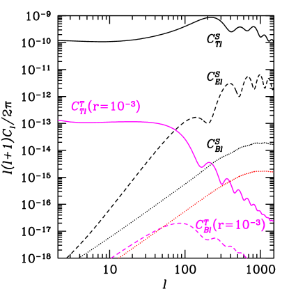
Figure 1: Angular power spectra. Solid lines are for temperature anisotropies due to scalar perturbations, $C_{Tl}^{S}$ and tensor perturbations, $C_{Tl}^{T}$ with $r=10^{-3}$. Dashed lines are for the E modes from scalar perturbations, $C_{El}^{S}$ and the B modes from tensor perturbations, $C_{Bl}^{T}$. The dotted lines are for the lensing–induced scalar B-modes, $C_{Bl}^{S}$ before (above) and after (below) the cleaning that can be done by a perfect experiment.

In Fig. 1 we show the angular power spectrum of CMB temperature perturbations contributed by scalar perturbations and by tensor perturbations with $r=10^{-3}$. By determining the total CMB temperature power spectrum we can determine or limit the energy scale of inflation, based on the presence or absence of extra power at low $l$. The scalar temperature perturbations inevitably limit our ability to detect the tensor temperature perturbations to those cases with $r>r_{\rm lim}=0.13$. knox94

In kamionkowski97 ; seljak97 it was pointed out that tensor perturbations result in CMB polarization patterns with a curl, whereas scalar perturbations do not. By analogy with electromagnetism, these modes are called “B-modes”, and the curl–free modes are called “E-modes”. This was an exciting development, because the new signature of tensor perturbations could not be confused with scalar perturbations. Figure 1 also shows the power spectrum of this B-mode with the amplitude it would have if $V_{*}^{1/4}=6.4\times 10^{15}$ GeV, corresponding to $r=10^{-3}$. It is a very weak signal, even at its peak $~{}10^{7}$ times less than the power spectrum of the temperature anisotropy. Ignoring any contaminating source of curl–mode polarization the detectability limit is solely a matter of sufficient sensitivity to the CMB polarization. For a detector of sensitivity $s$ uniformly observing the entire sky for time $t$:

$$r_{\rm lim}=10^{-2}\left({s\over\mu K\sqrt{\rm sec}}\right)^{2}\left({t\over 1~{}{\rm year}}\right)^{-1}.$$ (2)

Equation 2 kamionkowski98 does not take into account a contaminating source of B mode that arises from the lensing of the E mode by density perturbations along lines–of–sight between the observer and the last–scattering surface zaldarriaga98 . This scalar contribution to the B-mode power spectrum is shown in Fig. 1. As we will see below this contamination sets the detectability limit at $r_{\rm lim}=6\times 10^{-4}$, similar to what was found in lewis01 .

This lensing contaminant can be cleaned from the maps as discussed in hu01 ; hu02 . Here we show that there are limits to how well these maps can be cleaned. Our main result is that in the no–noise limit the tensor perturbations can be detected only if $V_{*}^{1/4}>3.2\times 10^{15}\,{\rm GeV}$. Interestingly, this is below the mass scale for the gauge coupling–constant convergence at $10^{16}\,{\rm GeV}$ that occurs in minimal extensions to the standard model of particle physics (e.g. langacker91 ).

The Stokes parameters, $I$, $Q$ and $U$ are related to the unlensed Stokes parameters (denoted with a tilde) by

$$I({\vec{\theta}})=\tilde{I}(\vec{\theta}+\delta\vec{\theta}) Q({\vec{\theta}})=\tilde{Q}(\vec{\theta}+\delta\vec{\theta}) U({\vec{\theta}})=\tilde{U}(\vec{\theta}+\delta\vec{\theta}).$$ (3)

The deflection angle, $\delta\vec{\theta}$, is the tangential gradient of the projected gravitational potential,

$$\phi({\vec{\theta}})=2\int dr{(r-r_{s})\over rr_{s}}\Psi(r\hat{n},r)$$ (4)

where $r$ is the coordinate distance along our past light cone, $s$ denotes the CMB last–scattering surface and $\hat{n}$ is the unit vector in the $\vec{\theta}$ direction.

The effect on the B–mode power spectrum is zaldarriaga98

$$C_{Bl}=C_{\tilde{B}l}+\sum_{l^{\prime}}W^{l^{\prime}}_{l}C_{\tilde{E}l^{\prime}}$$ (5)

where

$$W_{l}^{l^{\prime}}={l^{\prime 3}\over 4}\int_{0}^{\pi}\theta d\theta\times\{$$

$$\sigma_{2}^{2}(\theta)\left[J_{0}(l\theta)J_{2}(l^{\prime}\theta)-{1\over 2}J_{4}(l\theta)\left[J_{2}(l^{\prime}\theta)+J_{6}(l^{\prime}\theta)\right]\right]+$$

$$\sigma_{0}^{2}(\theta)\left[J_{4}(l\theta)J_{4}(l^{\prime}\theta)+J_{0}(l^{\prime}\theta)J_{0}(l\theta)\right]\}.$$ (6)

The functions $\sigma_{2}^{2}(\theta)$ and $\sigma_{0}^{2}(\theta)$ depend on the statistical properties of the displacement potential $\phi$ and are given by

$$\sigma_{0}^{2}(\theta) = \int{ldl\over 2\pi}l^{2}C_{l}^{\phi}(1-J_{0}(l\theta))$$

$$\sigma_{2}^{2}(\theta) = \int{ldl\over 2\pi}l^{2}C_{l}^{\phi}J_{2}(l\theta)$$ (7)

where

$$C_{l}^{\phi}\equiv\langle\phi_{lm}\phi_{lm}\rangle$$ (8)

and $\phi_{lm}$ is the spherical–harmonic transform of $\phi({\vec{\theta}})$.

If we have a means of determining $\phi$, and therefore $\delta\vec{\theta}$, we can reconstruct the unlensed maps from the lensed maps by use of Eq. 3. This procedure cleans out the lensing–induced B–mode. The $C_{l}^{\phi}$ above can either be interpreted as the power spectrum of the lensing potential (in the case of uncleaned maps in which case we will call it $C_{l}^{\phi(S)}$) or the power spectrum of the lensing potential residuals (in the case of lensing–cleaned maps). In the uncleaned case hu00 (in the Limber approximation valid at small scales):

$$C_{l}^{\phi(S)}={8\pi^{2}\over l^{3}}H_{0}^{2}\int_{0}^{r_{s}}drr\left[{(r-r_{s})\over rr_{s}}\right]^{2}\Delta_{\Phi}^{2}(k,r)|_{k=l/r}$$ (9)

where $r_{s}$ is the comoving distance to the last-scattering surface and $\Delta_{\Phi}^{2}(k,r)\equiv k^{3}/(2\pi)^{2}P_{\Phi}(k,r)$ where $P_{\Phi}(k,r)$ is the power spectrum of the gravitational potential at the time corresponding to coordinate distance $r$ on our past light cone. We plot $C_{l}^{\phi(S)}$ in Fig. 2

We consider the $\phi$ reconstruction procedure given in hu02 which exploits the fact that lensing leads to a mode–mode coupling with expectation value proportional to $\phi$. Their estimator is a minimum–variance (MV) average over pairs of map modes with $l\neq l^{\prime}$. Since we know the statistics of the signal, $C_{l}^{\phi}$, we can Wiener filter (WF) the MV estimate and further reduce the errors in the reconstruction. The error in the WF estimate of $\phi_{lm}$ has variance:

$$C^{\phi(WF)}_{l}={C^{\phi(S)}_{l}C^{\phi(MV)}_{l}\over C^{\phi(S)}_{l}+C^{\phi(MV)}_{l}}.$$ (10)

The Wiener–filtering is important in the low signal–to–noise regime $(C^{\phi(S)}_{l}/C^{\phi(MV)}_{l}\ll 1)$ where the variance of the reconstructed $\phi$ is $C^{\phi(S)}_{l}$ instead of $C^{\phi(MV)}_{l}$.

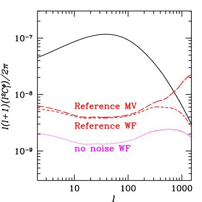
Figure 2: Angular power spectrum of projected gravitational potential, $\phi$ (solid curve) and the power spectrum of the residuals of different reconstruction procedures: minimum variance for “reference” experiment (long dashes), Wiener filter for the reference experiment (short dashes) and Wiener filter for a noiseless experiment (dotted line).

Cleaning can greatly reduce the amplitude of $C_{l}^{\phi}$ as is shown in Fig. 2 where the angular power spectrum of the residual $\phi$ is shown for two different experiments. The first is the ‘reference’ experiment of hu02 which makes temperature maps with weight-per-solid angle of $w=(1\mu{\rm K}-{\rm arcmin})^{-2}$ and $Q$ and $U$ maps each with half this weight, all with $7^{\prime}$ (full-width-half-maximum) resolution. The second is the no–noise, perfect angular resolution case. One can see that high signal–to–noise reconstruction of $\phi$ is possible.

Because the cleaning is not perfect, there is still lensing-induced scalar B-mode in the cleaned maps. In the no-noise limit the residual scalar B-mode power spectrum, $C_{Bl}^{WF}$, has been reduced by a factor of 10 from the uncleaned amplitude, as shown in Fig. 1.

Writing the tensor–induced B-mode power spectrum as $C_{Bl}^{T}=rC_{Bl}^{T,1}$ the resulting error in $r$, $\sigma_{r}$, is given by

$${1\over\sigma_{r}^{2}}=f_{\rm sky}\sum_{l}{2l+1\over 2}\left(C_{Bl}^{T,1}\right)^{2}\left(C_{Bl}^{WF}+w^{-1}e^{l^{2}\sigma_{b}^{2}}\right)^{-2}$$ (11)

where the $Q$ and $U$ maps cover $f_{\rm sky}$ of the sky with uniform weight per solid angle $w$ and have been smoothed by a circular Gaussian beam profile with full-width-half-maixmum = $\sqrt{8\ln 2}\sigma_{b}$. For $r_{\rm lim}=3.3\sigma_{r}$ we find for noise–free maps, but with no cleaning done, $r_{\rm lim}=6\times 10^{-4}$. For the ‘reference’ experiment of hu01 we find $r_{\rm lim}=4\times 10^{-4}$ after cleaning with the MV estimator and $1.8\times 10^{-4}$ with the WF estimator. Finally, for noise–free maps with WF cleaning $r_{\rm lim}=6\times 10^{-5}$.

All of the above results are for $f_{\rm sky}=1$. Given a detector (or array of detectors) with total sensitivity $s$ and an amount of observing time $t$ there is an optimal amount of sky to cover. Too much sky coverage means the maps are noisy and the lensing contaminant can not be removed accurately enough, too little sky hampers the statistical subtraction of the residual scalar B-mode power spectrum. The optimal sky coverage is given by $f_{\rm sky}^{\rm opt}=10^{-8}(\mu{\rm K})^{2}t/s^{2}$. In Fig. 3 we plot $r_{\rm lim}$ as a function of $s^{2}/t$ assuming optimal sky coverage (constrained to $f_{\rm sky}\leq 1$). The detectability limit is not strongly sensitive to deviations from optimal sky coverage, which is fortunate since other considerations can influence sky coverage choice as well. Note that $s^{2}/t=10^{-8}(\mu{\rm K})^{2}$ could be achieved by observing for a year with an array of 30,000 detectors each with sensitivity $100\mu{\rm K}\sqrt{\rm sec}$. Ten times more detectors (or integration time) are required to reach $s^{2}/t=10^{-9}(\mu{\rm K})^{2}$ and approach the smallest possible $r_{\rm lim}$. We have ignored aliasing of the scalar E–mode wich can be important for $f_{\rm sky}\neq 1$, as studied in lewis01 . Aliasing considerations increase $f_{\rm sky}^{\rm opt}$ and $r_{\rm lim}$. For $s^{2}/t=10^{-7}(\mu{\rm K})^{2}$ and $f_{\rm sky}=1$, $r_{\rm lim}=7\times 10^{-4}$. Therefore, including effects of aliasing would not increase $r_{\rm lim}$ by more than 40% over our results as shown in Fig. 3.

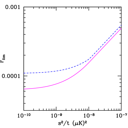
Figure 3: Achievable detectability limit as a function of total detector array sensitivity, $s$ and observing time $t$, assuming optimal sky coverage (lower curve) and 1/3 of optimal sky coverage (upper curve). Detectability limit assuming three times optimal sky coverage overlaps the upper curve when optimal sky coverage is less than 1/3.

Since we are interested in determining a fundamental limit to the detectability of tensor perturbations, undeterred by the virtual cost of imaginary experiments, we explore one further method of cleaning out the lensing contaminant. Imagine we reconstruct the projected gravitational potential or the density field on our past light cone out to some limiting redshift, $z_{\rm lim}$. Then we could directly calculate the lensing generated by the matter at $z<z_{\rm lim}$. Subtracting this lensing contaminant from CMB maps leaves only the contribution from $z>z_{\rm lim}$. The effect of this remaining lensing can be calculated by altering the lower limit of integration in Eq. 9 from 0 to $r(z_{\rm lim})$. To improve upon the noise–free self–cleaned maps result of $r_{\rm lim}=6\times 10^{-5}$ one needs to take $z_{\rm lim}\mathrel{\mathchoice{\lower 3.6pt\vbox{\halign{$\mathsurround=0pt\displaystyle\hfil#\hfil$\cr>\crcr\sim\crcr}}}{\lower 3.6pt\vbox{\halign{$\mathsurround=0pt\textstyle\hfil#\hfil$\cr>\crcr\sim\crcr}}}{\lower 3.6pt\vbox{\halign{$\mathsurround=0pt\scriptstyle\hfil#\hfil$\cr>\crcr\sim\crcr}}}{\lower 3.6pt\vbox{\halign{$\mathsurround=0pt\scriptscriptstyle\hfil#\hfil$\cr>\crcr\sim\crcr}}}}7$. We know of no way of obtaining this information at such high $z$.

Our analysis ignores polarized emission from galactic and extragalactic sources. Multi–frequency observations can be used to clean out these signals based on their distinct spectral shapes. However, even in the no–noise limit these cannot be cleaned perfectly since their spectral shapes are not perfectly well known and vary spatially (e.g. tegmark00b ). Our estimate of the detectability limit should be viewed as a lower limit.

How likely is it that the energy scale of inflation is high enough to be determined? It is conceivable that $V_{*}^{1/4}$ is as low as $10^{3}\,{\rm GeV}$knox93 . Given even odds between $10^{3}$ and $10^{19}$ GeV the chances are small. On the other hand gauge coupling unification gives us a hint that something interesting may be occurring at $10^{16}$ GeV. If inflation has anything to do with grand unification, or physics at higher energy scales, then the chances are good.

The likelihood of detection may also be addressed by better determination of the scalar spectrum. If we assume particular functional forms for $V(\phi)$ and a scalar perturbation spectrum with power–spectral index, $n$, near the scale–invariant value of unity, then we can give constraints on the range of possible values of $r$. Here we follow the nomenclature and calculations of dodelson97 . Exponential potentials have $r=5(1-n)$ and “small–field polynomial” potentials ($V(\phi)=\Lambda^{4}\left[1-\left(\phi/\mu\right)^{p}\right]$) with $p=2$ have $r=10\exp\left(-50\left(1-n\right)\right)$. Still other classes of models (hybrid inflation and the small–field polynomial potentials with $p>2$) leave little or no relationship between $r$ and $n$; $r$ can take on detectable values or vanishingly small ones. Perhaps the happiest case is the simplest one: polynomial potentials with $V(\phi)=\Lambda^{4}(\phi/\mu)^{p}$. With $p\geq 2$ all have $r>0.1$, well above our detectability limit.

In sum, we have calculated how large the amplitude of tensor perturbations must be in order for their effect on the CMB to be distinguishable from those of lensing. By reconstructing the lensing potential, using the mode–mode coupling induced by lensing, one can reduce the lensing contamination but not eliminate it. The residual lensing signal prevents detection of tensor perturbations if $V_{*}<(3.2\times 10^{15}\,{\rm GeV})^{4}$. If $V_{*}$ is slightly larger then an ambitious observational program may succeed in determining the energy scale of inflation—possibly a key step towards finding inflation a comfortable home in a fundamental theory of physics.

We thank A. Albrecht, D. Chung, N. Dalal and J. Kiskis for useful conversations. We used CMBfast seljak96 .

References

- (1) A. H. Guth, Phys. Rev. D23, 347 (1981).
- (2) A. Albrecht and P. J. Steinhardt, Physical Review Letters 48, 1220 (1982).
- (3) A. D. Linde, Physics Letters B 108, 389 (1982).
- (4) C. B. Netterfield et al., (2001), astro-ph/0104460.
- (5) A. T. Lee et al., Astrophys. J. Lett.561, L1 (2001).
- (6) N. W. Halverson et al., (2001), astro-ph/0104489.
- (7) U. Pen, U. Seljak, and N. Turok, Physical Review Letters 79, 1611 (1997).
- (8) B. Allen et al., Physical Review Letters 79, 2624 (1997).
- (9) A. Albrecht, R. A. Battye, and J. Robinson, Physical Review Letters 79, 4736 (1997).
- (10) J. Khoury, B. A. Ovrut, P. J. Steinhardt, and N. Turok, Phys. Rev. D64, 123522 (2001).
- (11) S. Dodelson, W. H. Kinney, and E. W. Kolb, Phys. Rev. D56, 3207 (1997).
- (12) M. S. Turner and M. White, Phys. Rev. D53, 6822 (1996).
- (13) L. Knox and M. S. Turner, Physical Review Letters 73, 3347 (1994).
- (14) M. Kamionkowski, A. Kosowsky, and A. Stebbins, Physical Review Letters 78, 2058 (1997).
- (15) U. . Seljak and M. Zaldarriaga, Physical Review Letters 78, 2054 (1997).
- (16) M. Kamionkowski and A. Kosowsky, Phys. Rev. D57, 685 (1998).
- (17) M. Zaldarriaga and U. Seljak, Phys. Rev. D58, 023003 (1998).
- (18) A. Lewis, A. Challinor, and N. Turok, (2001), astro-ph/0108251.
- (19) W. Hu, (2001), astro-ph/0108090.
- (20) W. Hu and T. Okamoto, (2001), astro-ph/0111606.
- (21) P. Langacker and M. Luo, Phys. Rev. D44, 817 (1991).
- (22) W. Hu, Phys. Rev. D62, 043007 (2000).
- (23) M. Tegmark, D. J. Eisenstein, W. Hu, and A. de Oliveira-Costa, Astrophys. J. 530, 133 (2000).
- (24) L. Knox and M. S. Turner, Physical Review Letters 70, 371 (1993).
- (25) U. Seljak and M. Zaldarriaga, Astrophys. J. 469, 437 (1996).
- (26) L. Knox, Phys. Rev. D52, 4307 (1995).
- (27) E. Bertschinger and A. Dekel, Astrophys. J. Lett.336, L5 (1989).