Are There Unstable Planetary Systems Around White Dwarfs?

Abstract

The presence of planets around solar-type stars suggests that many white dwarfs should have relic planetary systems. While planets closer than $\sim$ 5 AU will most likely not survive the post-main sequence lifetime of its parent star, any planet with semimajor axis $>$ 5 AU will survive, and its semimajor axis will increase as the central star loses mass. Since the stability of adjacent orbits to mutual planet-planet perturbations depends on the ratio of the planet mass to the central star’s mass, some planets in previously stable orbits around a star undergoing mass loss will become unstable. We show that when mass loss is slow, systems of two planets that are marginally stable can become unstable to close encounters, while for three planets the timescale for close approaches decreases significantly with increasing mass ratio. These processes could explain the presence of anomalous IR excesses around white dwarfs that cannot be explained by close companions, such as G29-38, and may also be an important factor in explaining the existence of DAZ white dwarfs. The onset of instability through changing mass-ratios will also be a significant effect for planetary embryos gaining mass in protoplanetary disks.

1 Introduction

The discovery of $\sim$ 80 planets, and counting, around solar type stars suggests that successful planet formation is quite common. The wealth of systems so unlike the Solar System leads one to conclude that many aspects of planetary system formation and dynamical evolution have yet to be fully explored. One particularly interesting area is the long term evolution of planetary systems specifically in the presence of post-main-sequence evolution of the central star. Observations of planets around post-main-sequence stars may provide additional information about the formation and evolution of planetary systems around main-sequence stars, and can inform us about the long term future of the solar system.

While planets at distances similar to the outer planets in the solar system will persist through post-main-sequence evolution (Duncan & Lissauer, 1998), it is unlikely that close Jovian companions to such stars survive. As the star evolves it expands, engulfing anything up to $\sim$ 1 AU (Sackmann et al., 1993; Siess & Livio, 1999a, b). Outwards of an AU, up to $\sim$ 5 AU any planet’s orbit will decay through tidal transfer of angular momentum and become consumed within the envelope of the star (Rasio et al., 1996). Anything with less mass than a brown dwarf will not survive in the stellar envelope (Livio & Soker, 1984; Soker et al., 1984).

Planets may still be observed in close orbits around white dwarfs if their orbits are significantly changed by some process that occurs after the AGB phase. If the planets become unstable to close approaches with each other, their interaction would result in a planet close to the central star, similar to scenarios proposed for the formation of close Jovian planets around main sequence stars (Rasio & Ford, 1996; Weidenschilling & Marzari, 1996; Lin & Ida, 1997). The results of close encounters between two Jovian planets have been studied in detail, with three possible outcomes: the two planets collide leaving a large planet, one planet is ejected, or both planets remain in a new stable configuration (Ford et al., 2001). For planets starting out with semi-major axes $>$ 5 AU, $\sim$8% of unstable pairs will collide, the remaining $\sim$92% will not. Of the systems which avoid collision, roughly 40% will settle into a configuration with a planet in a significantly closer and more eccentric orbit than in the initial system. Thus the onset of instability after post-main-sequence mass loss may create white dwarf systems with planets at obital radii scoured clear of the original inner planets during the star’s giant phase.

Duncan & Lissauer (1997), simulating the Uranian satellite system, found that Hill stable systems can become unstable with an increasing mass ratio for satellites orbiting a central massive object. This important work led to one of the few systematic studies of the post-main-sequence evolution of planetary systems dynamically similar to the solar system (Duncan & Lissauer, 1998). In that paper, Duncan & Lissauer found that the time to unstable close approaches for the planets followed a power-law relationship with the ratio of planetary mass to stellar mass, as an increasing fraction of mass was lost from the central star. At the level of individual planetary orbits, resonances may also play an important role in an adiabatically changing system, enhancing stability or creating instability. In this paper we generalize the specific results of Duncan & Lissauer (1998) to a range of system parameters applicable to a wider range of situations, such as those like the multi-planet extrasolar systems recently discovered.

Most likely, extrasolar planetary systems also possess Oort cloud analogues as a direct result of planet formation (Oort, 1950; Weissman, 1999). For comets in the outer Oort cloud orbital time scales are comparable to the more rapid late stages of post-main-sequence evolution, and the mass loss of a star is not adiabatic in the context of AGB evolution. If the mass loss is fairly symmetric, many of these comets survive the evolution and can later provide a steady flow of comets which impact the white dwarf directly, or break up due to tidal strain and populate the inner system with dust, causing photospheric metal contamination (Stern et al., 1990; Alcock, Fristrom, & Siegelman, 1986; Parriott & Alcock, 1998). However, if the planet systems become unstable to close approaches after the AGB phase, the entire system becomes dynamically young and new collisions and encounters can occur between surviving comets and planets. Many scenarios lead to a period of enhanced “late bombardment” as cometary orbits are perturbed and the flow of comets into the inner system is enhanced. In this paper we will investigate whether this mechanism can explain the observed IR excess around the white dwarf G29-38, attributed to a disk of dust whose extent is comparable to the tidal radius of the white dwarf (Graham, et al., 1990; Zuckerman & Becklin, 1987). Graham, et al. (1990) estimated that approximately 10¹⁵ g/yr of metal rich material would rain upon the white dwarf, if the infrared emission is due to a dust cloud at about half solar radius, requiring a steady and high rate of replenishment of the putative dust. Our model may resolve the problem of those DAZ white dwarfs which cannot be easily explained by either isolated cometary impacts or ISM accretion (Zuckerman & Reid, 1998).

We will show that the mass lost from a central star is sufficient to destabilize systems of two or more planets in previously stable orbits and cause them to suffer close approaches, producing several observable signatures. In section 2 we will develop the stability of planetary systems against close encounters in the presence of adiabatic mass loss, describe our numerical methods for testing our analytical estimates in section 3, present our results and discuss relevent observational signatures in section 4, and discuss the implications of these findings in section 5.

2 Stability for Planetary Systems Under Mass Evolution

2.1 Two Planet Systems

The stability of two planets against close approaches depends primarily on the masses of the planets relative to the central star and the separation of the two orbits. This separation is measured as $\Delta=(a_{2}-a_{1})/a_{1}$ where $a_{1}$ and $a_{2}$ are the inner and outer semi-major axes respectively. A critical Hill separation, $\Delta_{c}$ is then the minimum separation between two planets which ensures a lack of close approaches over all time (Hill, 1886). A full treatment of the Hill stability of two planets in the case of static masses can be found in Gladman (1993). Several approximations can be made that simplify the full treatment, such as equal planetary masses and small eccentricities. The criterion is then given by:

$$\Delta_{c}\simeq\sqrt{\frac{8}{3}\left(e^{2}_{1}+e^{2}_{2}\right)+9\mu^{2/3}}$$ (1)

where $\mu$ is the ratio of the planets’ mass to the central star, $e_{1}$, $e_{2}$ are the eccentricities of planet 1 and 2, and $\Delta_{c}$ is in units of the inner planet’s semi-major axis $a_{1}$.

If either the mass of the planets or the mass of the star changes, the critical Hill radius will change as well. An increase in planet mass or a decrease in stellar mass will cause $\mu$ to become larger, increasing the width of the zone in which orbits are unstable to close approaches. During post main-sequence mass loss, the orbits of planets will widen as the central star loses mass. As long as this process is adiabatic, the planets will simply conserve their angular momentum and widen their orbits proportionally to the mass lost: $a_{new}=a_{old}(M_{i}/M_{f})$. However, since the orbits widen together by the same factor, $\Delta$ remains the same. Thus, while the critical separation at which the two planets will become unstable widens, their relative separation remains unchanged. Orbits that are initially marginally stable, or close to being unstable, will become unstable to close planet–planet approaches as a consequence of the mass loss from the central star. In the case of planetary mass accretion in a protoplanetary disk, the orbits of the two planets will remain the same while $\Delta_{c}$ increases, creating the same effect as if the star were losing mass.

The opposite case of stellar mass accretion or planetary mass loss works to make previously unstable regions more stable. However, since close approaches generally happen within a few tens of orbits, objects likely would be cleared out of an unstable region quicker than the region could shrink.

2.2 Multiple Planet Systems

We expect that multiple planet systems should be common, e.g. the solar system, PSR 1257+12, and $\upsilon$ Andromedae (Wolszczan, 1994; Butler et al., 1999), and thus it is useful to develop an idea of how these systems remain stable. Chambers et al. (1996) found a relation between the separation of a system of planets and the time it would take for the system to suffer a close encounter:

$$\log{t}=b\delta+c$$ (2)

where $b$ and $c$ are constants derived through numerical simulations. The symbol $\delta$ is related to $\Delta$ but is defined in a slightly different way. Here, $\delta$ is the separation between two planets ($a_{i+1}-a_{i}$) in units of mutual Hill radii (R_i) defined as such:

$$R_{i}=\left(\frac{1}{3}\mu\right)^{1/3}\frac{\left(a_{i+1}+a_{i}\right)}{2}$$ (3)

where $i$ can be from 1 to $N_{planets}-1$ and we assume the planets have equal masses and initially circular orbits. If the parameter $\delta$ is the same for each pair of adjacent planets the separations in units of AU will be different. For example, if we took three Jovian mass planets ($\mu\sim 10^{-3}$) with $\delta=6.5$ and the innermost Jovian at 5.2 AU from the central star, the next two planets would be at 9.4 and 16.7 AU. Compare to actual orbital radii of 9.6 and 19.1 AU for Saturn and Uranus respectively, in our presumably stable for several billion years solar system. We add the obvious caveat that Saturn and Uranus are significantly less massive than Jupiter and have correspondingly weaker mutual interactions.

Adiabatic mass evolution will have the effect of shortening the time it takes for orbits to suffer close approaches. The knowledge of this has long been used to speed up numerical calculations (Duncan & Lissauer, 1997, and references therein). However, this fact also leads to the hypothesis that planetary systems on the edge of stability for 10¹⁰ yr will be affected by mass loss. In general the new time to close aproaches for an initial $\delta$ with a change in mass is given by:

$$\log{\frac{t_{f}}{t_{i}}}=(b^{\prime}-b)\delta+(c^{\prime}-c).$$ (4)

We would expect $c$ to have little or no change with a change of mass since it represents the timescale for two planets at $\delta\sim$0 to suffer a close approach. Mass loss will increase the mutual Hill radii of the planets which in turn will change $b$ to a new value we will define as $b^{\prime}$:

$$b^{\prime}=\left(\frac{\mu_{f}}{\mu_{i}}\right)^{\frac{1}{3}}b$$ (5)

where $\mu_{f}$ and $\mu_{i}$ are the final and initial mass ratios respectively. Such behavior suggests that bodies that are stable over the lifetime of a planetary system will become unstable over a timescale several orders of magnitude smaller than their original timescale for instability, when the central star becomes a white dwarf, assuming the relation of Equation 2 holds for large $\delta$. It has been found that for the case of three planets with $\mu$=10^-7, the parameters $b\simeq 1.176$ and $c\simeq-1.663$ (Chambers et al., 1996). If the three planets are each separated from their neighbor by $\delta$=6, they will experience close encounters after $\sim$10⁵ orbits of the inner planet. For comparison, three planets with the same mass ratio and separated by a $\delta=8$ will experience close encounters after $6\times 10^{7}$ yr. Assuming the central star loses half of its mass, the timescale to close encounters will shorten by an order of magnitude for the first case and two orders of magnitude for the second.

2.3 When is Mass Evolution Adiabatic?

The question of whether mass evolution is adiabatic needs to be addressed. In the case of mass loss for solar mass stars, roughly half the central star’s mass will be lost on the order of $10^{8}$ yr. A majority of the mass is lost at the tip of the AGB branch during a period of $\sim$10⁶ yr. Even the quickest rate of mass loss is much longer than one orbital period of a planet inwards of 100 AU, the general region where planets are believed to have formed. Stars heavier than a solar mass probably have superwinds which will cause significant mass loss on the order of a few hundred or thousand years (Vassiliadis & Wood, 1993; Schröder et al., 1999). Whether this is important or not will be the subject of further study. Objects very far away from the central star, such as Oort cloud object analogues, have orbital timescales comparable to the mass loss timescale and will also not follow the adiabatic case. It should be noted that for Kuiper and Oort cloud distances that the mass loss by the star would become adiabatic if the asymptotic wind velocity were orders of magnitude smaller than the escape velocity at the surface of the star since the crossing time of the wind would then be larger than the orbital timescale of the comets.

Mass gain of stars and planets is much slower than the orbital timescale of a planet. Accretion rates for protostars are on the order $10^{-6}$ M_⊙ yr^-1 (Shu et al., 1987). The formation of giant planets through runaway gas accretion takes $\sim$10⁷ yr, the rough lifetime of gaseous protoplanetary disks (Pollack et al., 1996). If some giant planets are formed more quickly by more efficient runaway accretion, gravitational collapse (Boss, 2000), or seeding through the formation of other planets (Armitage & Hansen, 1999), they would not be described by the adiabatic case.

3 Numerical Methods

In order to test the hypothesis that adiabatic mass evolution should change the stability of planetary systems, we ran several numerical simulations of two planet and multi-planet systems in circular orbits around a central star losing mass. The equations of motion were integrated using a Bulirsch-Stoer routine (Stoer & Bulirsch, 1980; Press et al., 1992). Since the case of mass loss of the central star and mass gain of the planet is the same, mass loss can be modeled in two ways. Either the star’s mass can be decreased, or the planets’ masses can be increased. If the planets’ masses are increased the time coordinate must be scaled to reflect the fact that the orbits are widening. To keep our investigations scalable, we chose the units of time to be orbits of the inner planet. We chose to increase the mass of the planets over a period of 1000 orbits. In the absence of mass evolution, energy and angular momentum were conserved to better than 1 part in 10⁶ for 10⁵ orbits. Since changng mass makes this a non-conservative system, energy and angular momentum could not be used as a test of accuracy. However, since the simulations were integrated until a close approach and then terminated, any error is similar to the case of no mass evolution. Several simulations without mass evolution were run with stable results. A close approach was defined by an encounter separated by a radius of $<$ 2$\mu^{2/5}$ (Gladman, 1993, and references therein). This radius was chosen because at separations smaller than this the planet-planet system is dominant and the star becomes a perturbation. Other authors have chosen different criteria (Chambers et al., 1996), but the results are insensitive to the exact choice.

In the two planet case, we started simulations at the critical separation predicted by Equation 1 assuming no mass loss, and increased the separation between the two planets at regular intervals in $\Delta$. We integrated the equations of motion until a close approach or for 10⁵ orbits. We increased $\Delta$ until it was 25% greater than what would be predicted in the presence of mass loss. These simulations were run an order of magnitude longer than Gladman (1993), and in the no mass loss case were consistent with what they found. The two planets were initially started with true anomalies separated by 180^∘. Our separations are then lower limits for the critical separation and thus truly reflect the minimum possible separation between orbits that remain stable. For multiple planets, $\delta$ was started at 2.2 and raised until several consecutive separations did not experience close encounters for 10⁷ orbits. Here random phases in the orbits where chosen with the restriction that adjacent orbits were separated by at least 40^∘. Three separate runs with different random initial phases were performed to improve the statistics for each mass, as there is significant scatter in the actual time to a close approach for each separation.

4 Results

4.1 Two Planets

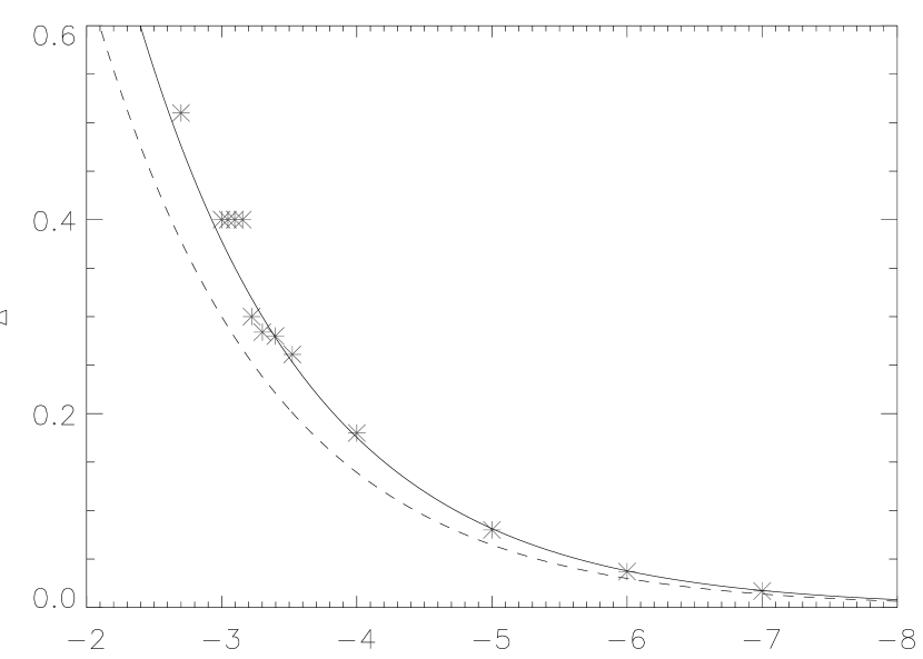
Figure 1: Results of several simulations of instability after mass loss. The dashed line corresponds to the original stability criterion of Equation 1. The solid line corresponds to the criterion with $\mu=2\mu_{i}$

We looked at a wide range of planetary masses for a solar mass star, from a sub terrestrial-sized planet ($\mu=10^{-7}$) to a Jovian planet ($\mu=10^{-3}$). Figure 1 shows the border for onset of instability in two planet systems after mass loss. The dashed line represents the initial critical Hill radius for no mass loss. The solid line which goes through the points is the critical Hill radius for $\mu$ equal to twice that of the initial system, corresponding to the planets doubling in mass or the central star losing half of its mass. Several of the higher mass points are greater than that predicted by the solid curve, an indication of higher order $\mu$ terms becoming important. It should be noted that these results are general to any combination of planet and stellar mass that have these ratios.

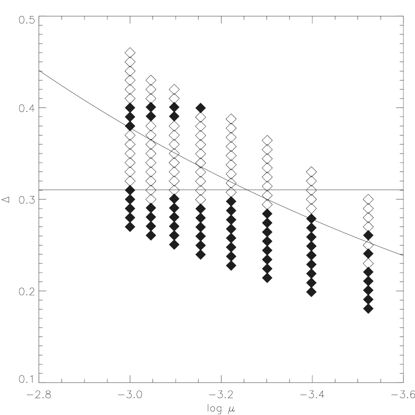
Figure 2: Close-up of Figure 1 in the range of 10^-3.5-10^-3. Open diamonds represent simulations that did not suffer any close approaches over 10⁵ orbits. Closed diamonds represent simulations that did suffer a close approach, while the solid curve represents the predicted $\Delta_{c}$ with mass loss. The horizontal solid line shows the relative separation that corresponds to the 3:2 resonance. A region of stability where instability is expected surrounds this resonance.

In a few cases, separations predicted to become unstable after mass loss by the Hill criterion were stable for the length of our simulations. Particularly in the $\mu$=10^-3 case, there was a large region in which the two planets suffered no close encounters (See Figure 2). These orbits corresponded to a range of $\Delta$ from .32 to .37, which were predicted to be unstable under mass evolution from the simple scaling of the equation for $\Delta$. It is interesting to note that all of these orbits are close to the 3:2 resonance (See Fig. 3). For the same reason that the Hill radius will not change, these orbits will retain the ratio of their periods. The reason for the stability around the 3:2 resonance may be due to those separations being near but not in a region of resonance overlap (Wisdom, 1980; Murray & Holman, 2001), clearly this conjecture needs to be confirmed but that goes beyond the scope of this particular paper.

4.2 Multiple Planets

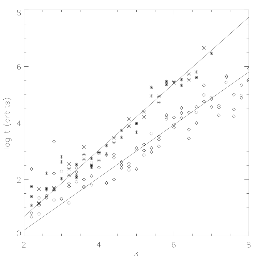
Figure 4: Comparison of the timescale to the first close approach for a system of three $\mu$=10^-7 planets with and without mass loss, where stars represent static masses and open diamonds represent the presence of mass loss. The top line is given by least-squares fitting a line of slope $b$ and intercept $c$ for no mass loss. The bottom line is given by Equation 5.

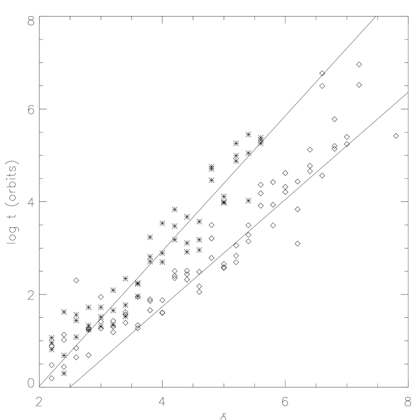
Figure 5: The $\mu=10^{-5}$ case, symbols the same as in Figure 4. The slope and intercept of the top line was derived by fitting the numerical simulations without mass loss. The slope of the bottom line is the predicted change due to mass loss.

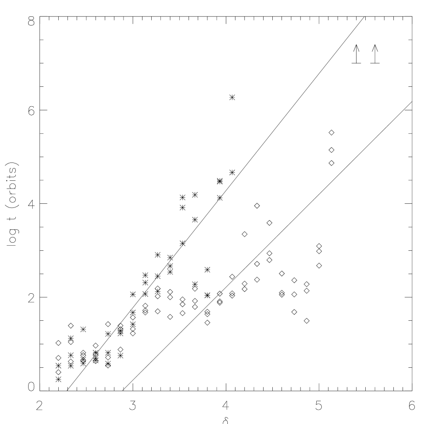
Figure 6: The $\mu$=10^-3 case, symbols the same as in Figure 4. The arrows indicate separations at which our simulations remained stable for 10⁷ orbits. The slope and intercept of the top line was derived by fitting the numerical simulations without mass loss. The presence of strong resonances is particularly noticeable as enhanced stability around $\delta$=5.2 for the mass loss case, which corresponds to the 2:1 resonance.

Figures 4-6 show the results for three different runs, looking at three planet systems in circular orbits. We looked at the mass ratios $\mu$=10^-7, 10^-5, and 10^-3. The results are compared to simulations without mass loss, and the difference between the two is quite noticeable for the whole range of mass. It is important to note that for separations whose time to close approach is comparable to the mass loss timescale show little change in behavior between the two cases. This is because the change in the time to close approach is smaller than the scatter in the simulations. Least squares fitting of the static and mass loss cases were performed to get the coefficients $b$, $c$, and $b^{\prime}$. To test our assumption of $c$ not changing under mass evolution, we also measured $c^{\prime}$, the intercept for the mass loss case. Planets with initial separations in $\delta$ that were less than $2\sqrt{3}$, the two planet stability criterion in units of $R_{i}$, were discarded. For the mass loss case, points where the timescale of close approaches were comparable to the mass loss timescale were also discarded. Once the coefficients were determined they were compared to what was predicted from Equation 2. Similarly, $b$ and $c$ from the $\mu$=10^-7 case without mass loss were compared with the results of Chambers et al. (1996). Table 1 shows that within the uncertainties, $c$ indeed does not change with mass evolution and the slopes are consistent with predictions. Additionally, our results for the static case with $\mu$=10^-7 are consistent with Chambers et al. (1996)’s values for $b$ and $c$.

As mass increases, the presence of strong resonances becomes more important. This is due to our choice of equal separations and equal masses, many of these resonances would disappear with small variations in mass, eccentricity, and inclination (Chambers et al., 1996), aspects that will be tested with further study. The presence of resonances is most easily seen in Figure 6 where $\mu$=10^-3. In the range of $\delta$=4.4 to 5.2, the points greatly depart from the predicted curve. the spike at $\delta$=5.2 corresponds to the first and second, as well as the second and third planets being in 2:1 resonances. This particular example shows that the basic dynamics of a system undergoing adiabatic mass evolution favor stability near strong resonances. Such a process potentially could augment the current ideas about how resonant extrasolar planets such as those around GJ876 formed (Snellgrove et al., 2001; Armitage et al., 2001; Murray et al., 2001; Rivera & Lissauer, 2000).

4.3 Observational Implications

These simulations have several observational implications which can be broadly separated into two categories–the character and the signature of planetary systems around white dwarfs.

Surviving planets that are marginally stable will suffer close approaches soon after the star evolves into a white dwarf, or possibly as early as the AGB phase. There are three possible end states for planets that suffer close approaches, ejection, collision, and a settling into a different and more stable configuration for all planets. The case of two planets has been studied carefully, and for two Jovian mass planets with one planet starting at $\sim$5 AU, the probability of collision is roughly 8%, ejection 35%, and rearrangement 57% (Ford et al., 2001). We naively assume that these results hold similarly for multiple planets as well, since collisions have been shown to hold for multiple planet systems (Lin & Ida, 1997), while ejections and rearrangements should have similar probability (certainly to within a factor of 2 or so). Ejections will leave planets that are closer to the white dwarf, while often a rearrangement will leave one or two planets with larger semi-major axes (up to $\sim$ 10³ times greater) and one with a smaller semi-major axis (as close as .1 times smaller). Collisions are potentially more exciting because as the two planets merge they essentially restart their cooling clock and as such will be anomalously luminous by 2 orders of magnitude for 10⁸ yr (Burrows et al., 1997).

To estimate how many white dwarfs might have planets that collided ($F_{c}$) we can take the fraction of white dwarfs that have marginally stable planets and multiply them by the fraction of marginally stable planets that have collisions:

$$F_{c}=f_{pl}f_{ms}f_{c}$$ (6)

where $f_{pl}$ is the fraction of white dwarfs with planets, $f_{ms}$ is the fraction of marginally stable planet systems, and $f_{c}$ is the fraction of marginally stable systems that suffer a collision. We can estimate the number of Jovian sized planets around white dwarfs by looking at the number of young stars that still have significant disks after 1 Myr, the approximate time to form a Jovian planet. This has been found to be about 50% of young stars in nearby clusters (Haisch, Lada, & Lada, 2001). Several numerical simulations (Barnes & Quinn, 2001; Laughlin & Adams, 1999; Quinlan, 1992; Rivera & Lissauer, 2000; Stepinski et al., 2000, for example,) point to a high frequency of marginally stable systems around stars as well as the discovery of the marginally stable planetary systems around GJ876 and HD 82943 (Marcy et al., 2001). However, factors such as multiple planets with widely different mass ratios could greatly change the effects of stability and need to be studied further. We estimate this fraction to be about 50% as well, although a large uncertainty is associated with this estimate. Taking the results above, we estimate then that $\sim 2(f_{ms}/0.5)$% of young white dwarfs should have the product of a recent planet-planet collision in orbit. Thus we predict that observations of young ($\tau\ll 10^{9}$ yr) white dwarfs should reveal $\sim 2$% have overluminous planet mass companions, some in orbits with semi-major axis smaller than the minimum (5 AU) expected to survive the AGB phase. These planets would be detectable through their significant IR excess, and should be distinguishable from brown dwarf companions.

A natural byproduct of the formation of Jovian planets is the existence of a large cloud of comets at large heliocentric distances (Oort, 1950; Weissman, 1999). The survival of such a cloud through post main-sequence evolution has been closely studied in the context of accounting for observed water emission in AGB stars and an explanation for metals in DA white dwarfs (Stern et al., 1990; Alcock, Fristrom, & Siegelman, 1986; Parriott & Alcock, 1998). The general result to date is that comets at semi-major axes greater than a few hundred AU survive the AGB phase. Then massive comets are predicted to strike the central white dwarf at a rate of $\sim 10^{-4}\,{\rm yr^{-1}}$, depositing fresh metals in the white dwarf photosphere. Such a cometary influx can account for the DAZ phenomenon, but has difficulty explaining some of the strongest metal line systems, because of the short predicted residence times of metals in the photosphere of these white dwarfs. An alternate explanation for the origin of metals in white dwarfs is ISM accretion, where a steady drizzle of metal rich dust is spherically accreted from the ambient ISM. Both scenarios have difficulty explaining the frequency of DAZ white dwarfs, and accounting for the systems with strongest metal lines and shortest residence times, due to the high mass accretion rate required to sustain those systems.

Recent observations of the DAZ phenomenon do not seem to be consistent with either scenario (Zuckerman & Reid, 1998). In one DAZ, G238-44, the diffusion time for metals is 3 days, which means that neither previous scenario can explain the high observed metal abundances nor the stability of the metal lines (Holberg, Barstow, & Green, 1997). Another white dwarf, G29-38, has a high abundance as well as an infrared excess, possibly from a dust disk at small orbital radii (Zuckerman & Becklin, 1987; Koester, Provencal, & Shipmann, 1997).

The evolution of a planetary system after post-main sequence mass loss coupled with the presence of an Oort cloud may provide an alternative explanation for the DAZ phenomenon and in particular the peculiarities of G29-38 and G238-44.

4.3.1 Cometary dynamics

The mass loss during post-main-sequence is near impulsive for Oort cloud comets. Previous work has shown that a significant fraction of any Oort cloud like objects will survive the mass loss phase, even in the presence of mildly asymmetric mass loss (Alcock, Fristrom, & Siegelman, 1986; Parriott & Alcock, 1998). The immediate result of the mass loss phase is to leave the remaining bound objects on orbits biased towards high eccentricity, but with similar initial periastrons. Orbital time scales are on the order of $10^{6}$ yr.

The number and typical size of Oort cloud objects is poorly constrained, canonical estimates scale to 1 km sized comets, mostly composed of low density ices and silicates, with masses of $\sim 10^{16}$ gm each, with order $10^{12}$ objects per star. Clearly there is a range of masses, and it is possible the true numbers and masses of Oort cloud comets vary by several orders of magnitude from star to star. Dynamical effects also lead to a secular change in the amount of mass in any given Oort cloud.

External perturbations ensure a statistically steady flux of comets from the outer Oort cloud into the inner system, where interactions with Jovian planets lead to tidal disruption of comets (and direct collisions), scattering onto tightly bound orbits restricted to the inner system, ejection from the system, and injection into central star encountering orbits. For the solar system, the flux of comets into orbits leading to collision with the Sun is of the order $10^{-2}$ per year, of these a significant fraction undergo breakup before colliding with the Sun, with individual fragments colliding with the Sun over many orbital periods (Kreutz sungrazers). SOHO detects $\sim 10^{2}$ such objects per year in the solar system, or one every 3 days or so on average. A single 1 km comet can fragment into $\sim 10^{4}$ fragments with sizes of order 50 m, consistent with those observed by SOHO, and consistent with the collision rates estimated both for the parent comets and the fragments. Each fragment then deposits about $10^{12}$ gm into the Solar photosphere. Note that if the typical comet were 20 km rather than 1 km, the deposition rate would be about $10^{16}$ gm every three days.

A white dwarf has a radius about 0.01 of the solar radius. Due to gravitational focusing, the cross-section for collision for comets scattered into random orbits in the inner system is linear in radius, so the collision rate expected for a white dwarf with a solar-like Oort cloud is $10^{-4}\,{\rm yr^{-1}}$. However, the perturbation of the outer orbits due to AGB mass loss, combined with the expansion of the outer planet orbits will drastically change this rate, leading to a new, late “heavy bombardment” phase with significantly higher rates of comet influx into the inner system. If one of the outer (Jovian mass) planets is scattered into a large ($a_{fin}\gg a_{in}$) eccentric orbit after the onset of instability, as we expect to happen in about 2/3 of the cases, then there will be strong periodic perturbations to the outer Kuiper belt and inner Oort cloud. About 10% of those systems will lead to the outermost bound planet being placed on very wide ($a_{fin}\mathrel{\raise 1.29167pt\hbox{$>$}\mkern-14.0mu\lower 2.58334pt\hbox{$\sim$}}10^{3}a_{in}$) highly eccentric orbits, with orbital time scales comparable to the cometary orbital timescales. Perturbations on the Oort cloud from these planets lead to a persistent high flux of comets to the inner system, until the Oort cloud is depleted of comets.

The net effect of the dynamical rearrangement of the post-main-sequence planetary system is a greatly enhanced rate of cometary influx into the inner system, starting $10^{7}$-$10^{8}$ years after the mass loss phase, tapering off gradually with time on time scales of $10^{8}$–$10^{9}$ years, leading to enhanced metal deposition to the white dwarf photosphere, and increased dust formation in the inner system for some white dwarfs, depending on the final configuration of the outer planets.

Several processes affect the comet bombardment rate:

• a fraction of the previously stably orbiting outer Kuiper belt objects, that survived the AGB phase, are injected into the inner system by newly established dynamical resonances with the outer planets over $\sim 10^{8}$ years;

• planets ejected to the outer Oort cloud by planet-planet perturbations will randomise the orbits of a small ($\sim 4(m/M)^{2}$) fraction of the Oort cloud comets, some of these will enter the inner system providing an enhanced flux of the normal Oort comet infall over $\sim 10^{9}$ years;

• surviving inner planets, scattered to the smaller orbital radius, will trap the comets injected into the inner system, providing both direct tidal disruption at a few AU, and providing a much higher influx of comets to very small radii where they are tidally disrupted by the white dwarf (or in rare cases collide directly);

• dust from tidally disrupted cometary debris will be driven to the white dwarf surface by PR drag, while larger debris will be dragged in through the Yarkovsky affect, both on a timescale shorter than the WD cooling time.

We expect the Kuiper belt to be severely depleted by the post-main-sequence phase (Stern et al., 1990; Meinick et al., 2001), however, a substantial population of volatile depleted rocky bodies may survive the AGB phase in the outer belt. A substantial fraction of these burnt out comets will become vulnerable to resonant perturbations by the surviving outer planets, now in new, wider orbits. The outer belt objects have orbital periods ($\sim 10^{4}$-$10^{5}$ years) that are becoming comparable to the most shortest AGB mass loss timescales, and therefore will not generally expand adiabatically in proportion to the expansion of the planetary orbits. The solar Kuiper belt is inferred to have $\sim 10^{5}$ objects with size above 100 km, assuming a mass function with approximately equal mass per decade of mass, characteristic of such populations, we infer a population of $\sim 10^{11}$ Kuiper belt objects with size of about 1 km, at an orbital radius of order $10^{3}$ AU. Order 1% of those will be vulnerable to the new dynamical resonances after the AGB phase, allowing for evaporative destruction and ejection, we estimate $\sim 10^{8}$ Kuiper belt objects will enter the inner system in the $10^{7}$-$10^{8}$ years after the AGB phase. The rate will peak at $\sim 10^{8}$ years and then decline as the reservoir of cometary bodies in orbits vulnerable to the new planetary resonances declines.

If there are multiple surviving Jovian planets, then the post-AGB planet-planet interactions will typically leave the inner planets on eccentric orbits, leading to broader resonances and a larger fraction of perturbed Kuiper belt objects. We expect in $\sim 2/3$ of the cases where there were multiple, initially marginally stable Jovian planets in the outer system, for the final configuration to have an eccentric outer planet, and a more tightly bound inner planet.

Some of the comets injected into the inner system will be tidally disrupted by the surviving Jovian planets, some will be ejected, and some will be injected into the inner system and be tidally disrupted by the white dwarf (and about 1% of those will directly impact the white dwarf). Dynamical time scales in the inner system are $\sim 10^{2}$ years, and the probability of ejection or disruption per crossing time is of the order of $10^{-2}$ per crossing time, assuming there is an inner planet, scattered inward of 5 AU, matching the outer planet scattered to wider orbital radius. So at any one time $\mathrel{\raise 1.29167pt\hbox{$>$}\mkern-14.0mu\lower 2.58334pt\hbox{$\sim$}}10^{3}$ Kuiper belt objects are in the inner system. The rate for tidal disruption by the surviving innermost Jovian planets is $\sim 10^{-6}\ {\rm yr^{-1}}$ per comet. Tidal disruption rates due to close approaches to the white dwarf may be as high as $\mathrel{\raise 1.29167pt\hbox{$>$}\mkern-14.0mu\lower 2.58334pt\hbox{$\sim$}}10^{-4}\ {\rm yr^{-1}}$ per comet, the rates are uncertain because of the possibility of non-gravitational processes breaking up the comet and deflecting debris. With each comet massing about $\mathrel{\raise 1.29167pt\hbox{$>$}\mkern-14.0mu\lower 2.58334pt\hbox{$\sim$}}10^{16}$ gm, by hypothesis, we get a flux of disrupted cometary material, from the Kuiper belt remnant, assuming solar system like populations, of $10^{14}$–$10^{16}$ gm per year. This is volatile depleted material, by hypothesis. Given our assumed mass function, disruption of rarer more massive comets can sustain mass accretion rates an order of magnitude higher still for time scales comparable to the inner system dynamical time scales, in a small fraction of systems.

We can now compare our mechanism to the accretion rates needed to explain the constant, detected metal lines in G29-38 and G238-44, two DAZ white dwarfs with the highest measured abundances of Ca. An accretion rate has already been quoted in the literature for G238-44, where $\sim 3\times 10^{17}\ {\rm g\ yr^{-1}}$ of solar abundance ISM would need to be accreted (Holberg, Barstow, & Green, 1997). In a volatile depleted case, only metals would be present converting to only $\sim 6\times 10^{15}\ {\rm g\ yr^{-1}}$ for cometary material. G29-38 also has a roughly estimated value of $\sim 1\times 10^{19}\ {\rm g\ yr^{-1}}$ corresponding to $\sim 2\times 10^{17}\ {\rm g\ yr^{-1}}$ in the volatile depleted case (Koester, Provencal, & Shipmann, 1997).

Both of these estimates were based on calculations made by Dupuis, Fontaine, & Wesemael (1993); Dupuis, Fontaine, Pelletier, & Wesemael (1993, 1992), who uses the ML3 version of mixing length theory. In fact, there are several other methods that can be used to model the convective layer of white dwarfs, including using other efficiencies of the ML theory and the CGM model of convection (Althaus & Benvenuto, 1998). The calculations differ by up to four orders of magnitude on the mass fraction $q$ of the convection layer’s base in white dwarfs with T_eff similar to G29-38. Taking values of $q$ for the base of the convection layer from Figures 4 and 6 in Althaus & Benvenuto (1998) and getting values for the diffusion timescale from tables 5 and 6 in (Paquette, et al., 1986) one can estimate what steady state accretion rate G29-38 requires for the different models. The smallest rate came from ML1 theory and the largest from ML3 theory, with CGM having an intermediate value, giving a range of $\sim 2\times 10^{13}\ {\rm g\ yr^{-1}}$ to $\sim 4.4\times 10^{17}\ {\rm g\ yr^{-1}}$. We favor the CGM value of $\sim 10^{15}\ {\rm g\ yr^{-1}}$, which is consistent with the estimate based on observations conducted by Graham, et al. (1990). The rate for G238-44 may be more robust due to the fact that convective models converge for hotter white dwarfs.

Both rates are consistent with our scenario if either white dwarf has two Jovian mass planets, one in a $\mathrel{\raise 1.29167pt\hbox{$>$}\mkern-14.0mu\lower 2.58334pt\hbox{$\sim$}}10$ AU, eccentric orbit, and another in a $\mathrel{\raise 1.29167pt\hbox{$<$}\mkern-14.0mu\lower 2.58334pt\hbox{$\sim$}}5$ AU orbit, after rearrangement. Alternatively, their progenitors had an order of magnitude richer Kuiper belt population than inferred for the Solar system. With a post-AGB age of $\sim 6\times 10^{8}$ years, and a mass of $\sim 0.7\>{\rm M_{\odot}}$, the original main sequence star of G29-38 was most likely more massive than solar and a more massive planetary and cometary system is not implausible. G238-44 is almost 10⁸ years old and would represent an object close to the peak of predicted cometary activity.

Our scenario may provide a consistent picture for the presence of DAZ white dwarfs and their anomalous properties (Zuckerman & Reid, 1998). We don’t expect all white dwarfs to have metal lines. Only about 2/3 of those which possessed marginally stable planetary systems containing two or more Jovians at orbital radii greater than $\sim 5$ AU will be able to generate significant late cometary bombardment from the outer Kuiper belt and inner Oort cloud. Following a similar estimate as in Equation 6, we predict about 14% of white dwarfs will be DAZs. Further, the rate will peak after $\sim 10^{8}$ years, after the planet-planet perturbations have had time to act, and then decline as the resevoir of perturbable comets is depeleted. The convective layer of the white dwarf will also increase by several orders of magnitude over time which would create a sharp drop of high abundance DAZs with decreasing T_eff. The drop would be greatest between 12000K and 10000K where the convective layer has its steepest increase (see fig. 4 of Althaus & Benvenuto (1998)). Zuckerman & Reid (1998), in conducting their survey of DAZ white dwarfs, estimated that $\sim$20% of white dwarfs were DAZ and that metal abundance dropped with T_eff sharply between 12000K and 8000K.

We expect DAZ white dwarfs to have potentially detectable (generally) multiple outer Jovian planets, whose orbits will show dynamical signatures of past planet-planet interaction, namely an outer eccentric planet, and an inner planet inside the radius scoured clean by the AGB phase.

5 Discussion

Using the above results we can compare the greatest fractional change in stability for two Jovian planets around different stars $>$ 1 M_⊙ that produce white dwarfs. We took the initial-final mass relation of (Weidemann, 2000) and calculated $\Delta_{c}$ without mass loss and with mass loss ($\Delta_{c}^{\prime}$). As can be seen in Figure 7, the higher the initial mass star, the greater the fractional change. This is expected, since higher mass stars lose more mass to become white dwarfs. The best candidates for unstable planetary systems would be higher mass white dwarfs, if planet formation is equally efficient for the mass range considered here. The scheme conjectured in this paper, provides a method for identifying and observing the remnant planetary systems of intermediate mass stars, which might otherwise be hard to observe during their main sequence life time.

One can predict the change in the critical separation where two planets will remain stable based on the change in $\mu$ over time, simply by differentiating $\Delta_{c}$ with time:

$$\frac{d\Delta_{c}}{dt}=\mu^{-2/3}\frac{d\mu}{dt}.$$ (7)

In the general case $d\mu/dt$ depends on two factors, the change in mass of the central star and the change in mass of the planets, given by

$$\frac{d\mu}{dt}=\mu\left(\frac{d\ln{M_{pl}}}{dt}-\frac{d\ln{M_{\star}}}{dt}\right).$$ (8)

For the critical separation to widen, $\mu$ must increase with time. Putting the two equations together gives the rate of change in $\Delta_{c}$:

$$\frac{d\Delta_{c}}{dt}=\mu^{\frac{1}{3}}\left(\frac{d\ln{M_{pl}}}{dt}-\frac{d\ln{M_{\star}}}{dt}\right).$$ (9)

The results of our multi-planet simulations are scalable to many situations, but for planet systems surviving around white dwarfs we are interested in timescales of $\sim$10¹⁰ yr for solar type stars to $\sim$10⁸ yr for higher mass stars. The highest $\delta$ we studied for $\mu$=10^-3 was roughly 5.2, which by Equation 2 corresponds to a timescale to close approaches of 10⁷ orbits of the inner planet. After the central star loses half of its mass, the timescale shortens to $\sim$2000 orbits. For a planetary system with $\delta$=5.2 to be stable over the main sequence lifetime of the star, the minimum semimajor axis of the innermost planet for a higher mass star (say, 4M_⊙) would be 8.2 AU and 100 AU for a solar-type star. Longer integrations need to be performed to investigate the behavior of systems with larger values of $\delta$. We expect our results for time scales for onset of instability to scale to larger $\delta$, the initial computational effort we made here limited the exploration of slowly evolving systems with large $\delta$ in exchange for a broader exploration of the other initial condition parameters. It will also be instructive to model systems with unequal mass planets, to explore the probability of ejection and hierarchical rearrangement as a function of planetary mass ratio.

By performing numerical integrations of two planet and multiple planet systems we have shown that the stability of a system changes with mass evolution. In the specific case of mass loss as the central star of a planetary system becomes a white dwarf, we have found that previously marginally stable orbits can become unstable fairly rapidly after the mass loss process. Coupled with our knowledge of the survival of material exterior to outer planets such as Kuiper Belt and Oort Cloud analogues (Stern et al., 1990), a picture of the evolution of circumstellar material over the latter stages of a star’s lifetime becomes clear.

As a star reaches the RGB and AGB phases, inner planets are engulfed by both the expanding envelope of the star and through tidal dissipation. The surviving planets move slowly outwards, conserving their angular momentum as the star loses its mass over several orbital periods of the planets. The planets may sculpt the resulting wind of the giant star (Soker, 2001) and if they are on the very edge of stability undergo chaotic epsiodes during the AGB phase, creating some of the more exotic morphologies in the resulting planetary nebula. When the star becomes a white dwarf, two planet systems that are marginally stable will become unstable and suffer close approaches, while for three or more planets the timescale to close approaches shortens by orders of magnitude. There are three possible outcomes once the planets start suffering close approaches: the planets collide, one planet is ejected, or the two planets remain but are in highly eccentric orbits (Ford et al., 2001). One major open question is how many marginally stable systems there are, but there are indications that many, if not most, general planetary systems should be close to instability (Barnes & Quinn, 2001; Laughlin & Adams, 1999; Quinlan, 1992; Rivera & Lissauer, 2000; Stepinski et al., 2000) Rocky material in the inner edge of the Kuiper Belt, which is defined by the last stable orbits with respect to the planetary system, will follow the same fate as marginally stable planets, suffering close approaches with the planetary system and becoming scattered into the inner system, which increases the rate of close encounters with the planets or the central white dwarf. The surviving material at outer Kuiper Belt and Oort Cloud distances will have orbital periods comparable to the timescale of the central star’s mass loss. These objects have their eccentricity pumped up by the effectively instantaneous change in the central star’s mass, and then through interactions with planets create a new dust disk around the white dwarf, and contaminate the white dwarf photosphere to an observable extent.

The sensitivity of stability to changes in mass has implications for planet formation as well. Further research on the migration of Hill stable regions while the planet/star mass ratio evolves may illuminate further the general issue of how Jovian planets in the process of formation become unstable to close encounters and gross changes in orbital parameters (Ford et al., 2001). One possibility is that the mass accretion of the planets occurs at a rate fast enough that d$\mu/dt>0$. Other factors would need to be considered, in particular the interplay between the onset of rapid mass accretion by the planet, and the accretion rate from the protoplanetary disk onto the central protostar. Gas drag and stellar mass accretion could work to stabilize orbits if the planets are embedded in a circumstellar disk, while orbital migration would change the relative separations of proto-planets. Since the stability of multi-planet systems is also sensitive to changes in mass ratio, this could help solve problems of isolation for planetary embryos and speed up the timescale for the production of giant planet cores.

The dependence of stability on both the mass of the planet and the mass of the central star suggests that stars of different masses may be more efficient at producing a certain size planet. This is exemplified by the fact that $\mu$ for a Jovian planet can change by an order of magnitude in either direction over the mass range of stars that might have planetary companions. For larger mass stars, planets can be more tightly spaced and still be mutually dynamically stable, which suggests that when planets are forming it is easier for them to become dynamically isolated in disks around more massive protostars. For lower mass stars, there is a wider annulus in which material is unstable to planetary gravitational perturbations, and so forming planets would have a larger reservoir of material to draw from. Other factors that need further research would play into this result as well and may dominate over this scenario, such as a star’s temperature and radiation pressure. However, such effects will tend to reinforce the conclusion that less massive stars should be more efficient at creating more massive planets while higher mass stars will produce more, lighter planets if they are capable of forming planets at all. This prediction will be testable as many space and ground based programs are devoting a great deal of effort to look for planetary companions to stars.

Figure 3: Orbits around the 3:2 resonance for two planet stability. The top and bottom lines correspond to orbits that end in a close approach while the middle line shows an orbit that was stable over the length of the simulations.

Figure 7: Comparison of $\Delta_{c}$ with and without mass loss as a function of the central star’s original mass. The right figure shows the fractional change of $\Delta_{c}$ when mass loss occurs. For both figures the fractional change in mass is calculated using the M_i-M_f relation of Weidemann [2000].

References

- Alcock, Fristrom, & Siegelman [1986] Alcock, C., Fristrom, C. C., & Siegelman, R. 1986, ApJ, 302, 462
- Althaus & Benvenuto [1998] Althaus, L. G. & Benvenuto, O. G. 1998, MNRAS, 296, 206
- Armitage & Hansen [1999] Armitage, P. J. & Hansen, B. M. S. 1999, Nature, 402, 633
- Armitage et al. [2001] Armitage, P. J. et al. 2001, preprint (astro-ph/0104400)
- Barnes & Quinn [2001] Barnes, R. & Quinn, T. 2001, ApJ, 550, 884
- Boss [2000] Boss, A. P. 2000, ApJ, 536, L101
- Butler et al. [1999] Butler, R. P. et al. 1999, ApJ, 526, 916
- Burrows et al. [1997] Burrows, A. et al. 1997, ApJ, 491, 856
- Chambers et al. [1996] Chambers, J. E., Wetherill, G. W., & Boss, A. P. 1996, Icarus, 119, 261
- Chu et al. [2000] Chu, Y. et al. 2001, ApJ, 546, L61
- Delfosse et al. [1998] Delfosse, X. et al. 1998, A&A, 338, L67
- Duncan & Lissauer [1997] Duncan, M. J. & Lissauer, J. J. 1997, Icarus, 125, 1
- Duncan & Lissauer [1998] Duncan, M. J. & Lissauer, J. J. 1998, Icarus, 134, 303
- Dupuis, Fontaine, & Wesemael [1993] Dupuis, J., Fontaine, G., & Wesemael, F. 1993, ApJS, 87, 345
- Dupuis, Fontaine, Pelletier, & Wesemael [1993] Dupuis, J., Fontaine, G., Pelletier, C., & Wesemael, F. 1993, ApJS, 84, 73
- Dupuis, Fontaine, Pelletier, & Wesemael [1992] Dupuis, J., Fontaine, G., Pelletier, C., & Wesemael, F. 1992, ApJS, 82, 505
- Ford et al. [2001] Ford, E. B., Havlickova, M., & Rasio, F. A. 2001, Icarus, 150, 303
- Gladman [1993] Gladman, B. 1993, Icarus, 106, 247
- Graham, et al. [1990] Graham, J. R., Matthews, K., Neugebauer, G., & Soifer, B. T. 1990, ApJ, 357, 216
- Griffin et al. [2000] Griffin, R. E. M., David, M., & Verschueren, W. 2000, A&AS, 147, 299
- Haisch, Lada, & Lada [2001] Haisch, K. E., Lada, E. A., & Lada, C. J. 2001, ApJ, 553, L153
- Hill [1886] Hill, G. W. 1886, Acta Math., 8, 1
- Holberg, Barstow, & Green [1997] Holberg, J. B., Barstow, M. A., & Green, E. M. 1997, ApJ, 474, L127
- Kepler et al. [1990] Kepler, S. O. et al. 1990, ApJ, 357, 204
- Kleinman et al. [1994] Kleinman, S. J. et al. 1994, ApJ, 436, 875
- Koester, Provencal, & Shipmann [1997] Koester, D., Provencal, J., & Shipmann, H. L. 1997, A&A, 320, L57
- Kuchner et al. [1998] Kuchner, M. J., Koresko, C. D., & Brown, M. E. 1998, ApJ, 508, L81
- Laughlin & Adams [1999] Laughlin, G. & Adams, F. C. 1999, ApJ, 526, 881
- Lin & Ida [1997] Lin, D. N. C. & Ida, S. 1997, ApJ, 477, 781
- Livio & Soker [1984] Livio, M. & Soker, N. 1984, MNRAS, 208, 763
- Marcy et al. [2001] Marcy, G. W., Butler, R. P., Fischer, D., Vogt, S. S., Lissauer, J. J., & Rivera, E. J. 2001, ApJ, 556, 296
- Meinick et al. [2001] Meinick, G.J. Neufeld, D.A., Saavik Ford, K.E., Hollenbach, D.J., & Ashby, M.L.N. 2001, Nature, 412, 160
- Murray et al. [2001] Murray, N., Paskowitz, M. , & Holman, M. 2001, preprint (astro-ph/0104475)
- Murray & Holman [2001] Murray, N. & Holman, M. 2001, Nature, 410, 773
- Oort [1950] Oort, J. H. 1950, Bull. Astron. Inst. Netherlands, 11, 91
- Paquette, et al. [1986] Paquette, C., Pelletier, C., Fontaine, G., & Michaud, G. 1986, ApJS, 61, 197
- Parriott & Alcock [1998] Parriott, J. & Alcock, C. 1998, ApJ, 501, 357
- Pollack et al. [1996] Pollack, J. B. et al. 1996, Icarus, 124, 62
- Press et al. [1992] Press, W. H. et al. 1992, Numerical Recipes in Fortran. (2nd Edition; New York: Cambridge University Press)
- Quinlan [1992] Quinlan, G. D. 1992, IAU Symp. 152: Chaos, Resonance, and Collective Dynamical Phenomena in the Solar System, 152, 25
- Rasio & Ford [1996] Rasio, F. A. & Ford, E. B. 1996, Science, 274, 954
- Rasio et al. [1996] Rasio, F. A. et al. 1996, ApJ, 470, 1187
- Rivera & Lissauer [2000] Rivera, E. J. & Lissauer, J. J. 2000, ApJ, 530, 454
- Sackmann et al. [1993] Sackmann, I. Boothroyd, A. I., & Kraemer, K. E. 1993, ApJ, 418, 457
- Schröder et al. [1999] Schröder, K. Winters, J. M., & Sedlmayr, E. 1999, A&A, 349, 898
- Shu et al. [1987] Shu, F. H., Adams, F. C., & Lizano, S. 1987, ARA&A, 25, 23
- Siess & Livio [1999a] Siess, L. & Livio, M. 1999, MNRAS, 304, 925
- Siess & Livio [1999b] Siess, L. & Livio, M. 1999, MNRAS, 308, 1133
- Snellgrove et al. [2001] Snellgrove, M. D. Papaloizou, J. C. B. , Nelson, & R. P. 2001, preprint (astro-ph/0104432)
- Soker [2001] Soker, N. 2001, MNRAS, 324, 699
- Soker [1999] Soker, N. 1999, MNRAS, 306, 806
- Soker et al. [1984] Soker, N., Livio, M., & Harpaz, A. 1984, MNRAS, 210, 189
- Stepinski et al. [2000] Stepinski, T. F., Malhotra, R., & Black, D. C. 2000, ApJ, 545, 1044
- Stern et al. [1990] Stern, S. A., Shull, J. M., & Brandt, J. C. 1990, Nature, 345, 305
- Stoer & Bulirsch [1980] Stoer, J. Bulirsh, R. 1980,Introduction to Numerical Analysis (New York: Springer-Verlag)
- Vassiliadis & Wood [1993] Vassiliadis, E. & Wood, P. R. 1993, ApJ, 413, 641
- Weidemann [2000] Weidemann, V. 2000, A&A, 363, 647
- Weidenschilling & Marzari [1996] Weidenschilling, S. J. & Marzari, F. 1996, Nature, 384, 619
- Weissman [1999] Weissman, P. R. 1999, Space Science Reviews, 90, 30
- Wisdom [1980] Wisdom, J. 1980, AJ, 85, 1122
- Wolszczan [1994] Wolszczan, A. 1994, Science, 264, 538
- Zuckerman & Becklin [1987] Zuckerman, B. & Becklin, E. E. 1987, Nature, 330, 138
- Zuckerman & Reid [1998] Zuckerman, B. & Reid, I. N. 1998, ApJ, 505, L143