Evolution and structure of magnetic fields in simulated galaxy clusters

We use cosmological magneto-hydrodynamic simulations to study the evolution of magnetic fields in galaxy clusters in two different cosmological models, a standard-CDM and a $\Lambda$-CDM model. We show that the magnetic field strength profiles closely follow the cluster density profiles outside a core region of radius $\sim 200h^{-1}\,\mathrm{kpc}$. The magnetic field has a correlation length of order $50h^{-1}\,\mathrm{kpc}$ and reverses on scales of $\sim 100h^{-1}\,\mathrm{kpc}$ along typical lines-of-sight. The power spectrum of the magnetic field can well be approximated by a steep power law with an exponent of $\sim-2.7$. The mean magnetic field in the cluster cores grows roughly exponentially with decreasing redshift, $B\sim 10^{-2.5z}\,\mu\mathrm{G}$. Merger events have a pronounced effect on magnetic field evolution, which is strongly reflected in measurable quantities like the Faraday rotation. The field evolution in the two different cosmologies proceeds virtually identically. All our cluster models very well reproduce observed Faraday rotation measurements when starting with nG seed fields.

1 Introduction

While Faraday-rotation measurements clearly show that galaxy clusters contain magnetic fields which are smooth on scales of order $100h^{-1}\,\mathrm{kpc}$, their origin and their evolution are largely unclear. Fields of that scale must be related to the formation and evolution of the host cluster rather than the kinematics and internal evolution of the cluster galaxies. It is therefore an interesting question in what way galaxy clusters deform, compress and amplify the seed fields pervading the material that finally ends up in cluster cores, what magnetic field configurations are prevalent in final, virialised clusters, and whether the cosmological background model has any significant effect on the evolution of intracluster fields.

We address these questions with cosmological, magnetohydrodynamic cluster simulations. The numerical code used for this study uses smooth-particle hydrodynamics (SPH) for the magnetised intracluster gas and purely gravitational interaction between the particles of the dominant dark-matter component. The technical and numerical properties of our “Grape-MSPH” code, its performance in various tests, and results of a first application to cluster evolution were described in an earlier paper (Dolag et al. 1999). Here, we extend this earlier study in several ways. First, we perform cluster simulations in two different cosmological models, a standard-CDM (SCDM) model with $\Omega=1$ and $\Lambda=0$, and a $\Lambda$CDM model with $\Omega=0.3$ and $\Lambda=0.7$, to explore the influence of the cosmological background model. Second, we focus on the structure of the intracluster magnetic fields, quantified by radial field-strength profiles, correlation and field-reversal lengths, and the magnetic-field power spectrum. Third, we investigate how magnetic fields grow during cluster evolution, and how they are affected by cluster mergers. Finally, we compare the Faraday rotation predicted by our cluster models with the largest available sample of Faraday-rotation measurements.

2 Numerical technique and initial conditions

2.1 GrapeMSPH

Our cosmological MHD code “Grape-MSPH” was described in detail in Dolag et al. (1999). Therefore, we only give a brief summary here. The code combines the merely gravitational interaction of a dominant dark-matter component with the hydrodynamics of a magnetised gaseous component. The gravitational interaction of the particles is evaluated on GRAPE boards (cf. Sugimoto et al. 1990), while the gas dynamics is computed in the SPH approximation (Lucy 1977; Monaghan 1992). The original “GrapeSPH” code (Steinmetz 1996) was augmented by an implementation of the (ideal) magneto-hydrodynamic equations describing the evolution of the magnetic fields carried by the gas. Throughout, we assume that the electric conductivity of the gas is infinite, which implies that the magnetic fields are frozen into the gas flow. The back-reaction of the magnetic fields on the gas via the Lorentz force is fully included. The numerical viscosity required by SPH to properly capture shocks is chosen such that angular-momentum transport in presence of shear flows is carefully controlled. The SPH kernel width is automatically adapted to the local number density of SPH particles, which results in an adaptive spatial resolution of the code.

Extensive tests of the code were performed and described in Dolag et al. (1999). The code succeeds in solving the co-planar MHD Riemann problem posed by Brio & Wu (1988). Although the simulated magnetic field is not strictly divergence-free, monitoring shows that $\nabla\cdot\@vec{B}$ always remains negligible compared to the magnetic field divided by a typical length scale of $\@vec{B}$ (see Dolag et al. (1999) for more detail). The code also assumes the intracluster medium to be an ideal gas with an adiabatic index of $\gamma=5/3$. Although foreseen and implemented in the code, we neglect cooling here. One reason is that we cannot avoid the cooling catastrophe without a substantial source of heat. Most of the gas cools and ends up in an unphysically condensed central lump. Moreover, the cool gas fraction strongly depends on the resolution of the simulation. In addition, a substantial amount of numerical heating is expected due to our limited mass resolution.

The surroundings of the clusters are important because their gravitational tidal fields affect the overall cluster structure and the merger history of the clusters during formation. Therefore, the cluster simulation volumes are surrounded by a layer of boundary particles whose purpose it is to accurately represent the tidal fields of the cluster neighbourhood.

model	$H_{0}$	$\Omega_{\mathrm{m}}^{0}$	$\Omega_{\Lambda}^{0}$	$\sigma_{8}$	$f_{\mathrm{bary}}$	Source
SCDM	0.5	1.0	0.0	1.2	5%	(1)
$\Lambda$CDM	0.7	0.3	0.7	1.05	10%	(2)

Table 1: Parameters of the SCDM and the $\Lambda$CDM model. The SCDM clusters are COBE normalised, which is in conflict with the local cluster abundance. However, this does not affect our specific results because we are studying the magnetic field growth in individual clusters. Initial conditions are kindly provided by: (1) Bartelmann & Steinmetz 1996, (2) Eke et al. 1998.

2.2 Initial conditions

We set up initial conditions for two CDM-dominated model universes (standard CDM, SCDM; and flat, low-density CDM, $\Lambda$CDM), whose parameters are listed in Table 1. For the SCDM models, the central region of $\sim 70\,{\rm Mpc}$ (comoving) are filled with dark-matter particles with a mass of $3.2\times 10^{11}\,M_{\odot}$ each, mixed with an equal number of gas particles whose mass is twenty times smaller. The central region is surrounded by collisionless boundary particles whose mass increases outward to mimic the tidal forces of the neighbouring large-scale structure. Including the region filled with boundary particles, the simulation volume is a sphere with a (comoving) diameter of $\sim 300\,{\rm Mpc}$. For the $\Lambda$CDM models, the dark matter particles have masses of $8.1\times 10^{10}\,M_{\odot}$ each, while the mass of the gas particles is ten times smaller. Including the region filled with boundary particles, the simulation volume in this case has a comoving diameter of $\sim 600\,{\rm Mpc}$. The simulations labelled as “double” are taken from the SCDM models, but have twice the number of particles with half the original mass. For each cosmology, we used ten different realisations of the density-fluctuation field at an initial redshift $z_{\mathrm{ini}}=15$ (SCDM, kindly provided by M. Steinmetz) and $z_{\mathrm{ini}}=20$ ($\Lambda$CDM, kindly provided by J. F. Navarro). Note that the growth of fluctuations is slowed down in a $\Lambda$CDM model compared to the SCDM model. The different initial redshifts compensate for that, so that the initial fluctuations in linear expectation grow by the same amount in both cosmologies.

Each of these realisations evolves such that it contains clusters of different final masses and in different dynamical states at the final redshift $z=0$. We simulate each of these clusters with up to five different initial configurations of the magnetic field, which are listed in Table. 2. In addition, one set (SCDM) is computed with its mass resolution increased by a factor of two to test for resolution effects in our results. In total, we simulate and study 100 cluster models.

model	$B_{\mathrm{ini}}$	$\langle B_{\mathrm{final}}\rangle_{\mathrm{core}}^{\mathrm{SCDM}}$	$\langle B_{\mathrm{final}}\rangle_{\mathrm{core}}^{\Lambda\mathrm{CDM}}$
low	$0.2\times 10^{-9}\,{\rm G}$	$0.4\;\mu{\rm G}$	$0.3\;\mu{\rm G}$
chaotic	$0.2\times 10^{-9}\,{\rm G}$	$0.4\;\mu{\rm G}$	—
double	$0.2\times 10^{-9}\,{\rm G}$	$1.0\;\mu{\rm G}$	—
medium	$1.0\times 10^{-9}\,{\rm G}$	$1.1\;\mu{\rm G}$	$0.8\;\mu{\rm G}$
high	$5.0\times 10^{-9}\,{\rm G}$	$2.5\;\mu{\rm G}$	$2.0\;\mu{\rm G}$

Table 2: Initial magnetic fields (Col. 2) and the resulting final mean magnetic field strengths in the cluster cores (Cols. 3 and 4 for SCDM and $\Lambda$CDM models, respectively). The final values are an average over the gas particles central region (enclosed by a radius of $0.1\,r_{\mathrm{v}ir}$) across the sample of ten clusters simulated for each cosmology. Note that in the case of doubled mass resolution, the amplification of the initial field is significantly increased because shear flows are better resolved. This means that the initial field required to reproduce the observations with our simulations are only upper limits. Apart from that, there is no indication that the increased resolution changes the characteristics of the final magnetic field.

Lacking any detailed knowledge on the origin of primordial magnetic seed fields, we explore two extreme cases of initial field configurations. In one case (“homogeneous”), we assume that the field is initially constant throughout the cluster volume. In the other case (“chaotic”), we let the initial field orientation vary randomly from place to place, subject only to the condition that $\nabla\cdot\@vec{B}=0$. The initial field strengths in both cases are determined by setting the mean field energy densities. To study the effects of changing the mean initial energy density of the magnetic seed field, we ran simulations using three choices for this quantity, labelled “low”, “medium” and “high”.

To gain some insight into performance of the numerics, we also ran a set of simulations with doubled mass resolution, labelled “double”. The magnetic field configurations of these runs are the same as in the “homogeneous” case. Of course, this is not meant to replace a full resolution study. Here, we are limited by the capacity of our GrapeMSPH code, because the Grape design restricts the number of gas particles. We also ran a set of control simulations for each cosmological model without magnetic field, labelled “no”. In total, we have a set of ten realisations for each cosmology, simulated with six different magnetic field setups in the SCDM cosmology, and with four different magnetic field setups in the $\Lambda$CDM cosmology, leading to the 100 simulated clusters mentioned before.

Table 2 summarises the initial field set-ups and the mean field strengths in the cluster cores. The initial field strengths are of order $10^{-9}\,$G, the final field strengths of micro-Gauss order are averaged over the gas particles within spheres of $0.1\,r_{\mathrm{v}ir}$ and across the sample of ten clusters. For some aspects of the analysis of the simulations to be described later on, we also use ten less massive objects identified close to the main clusters. As they are relatively more poorly resolved in the simulations, the results from this smaller objects have to be treated with caution.

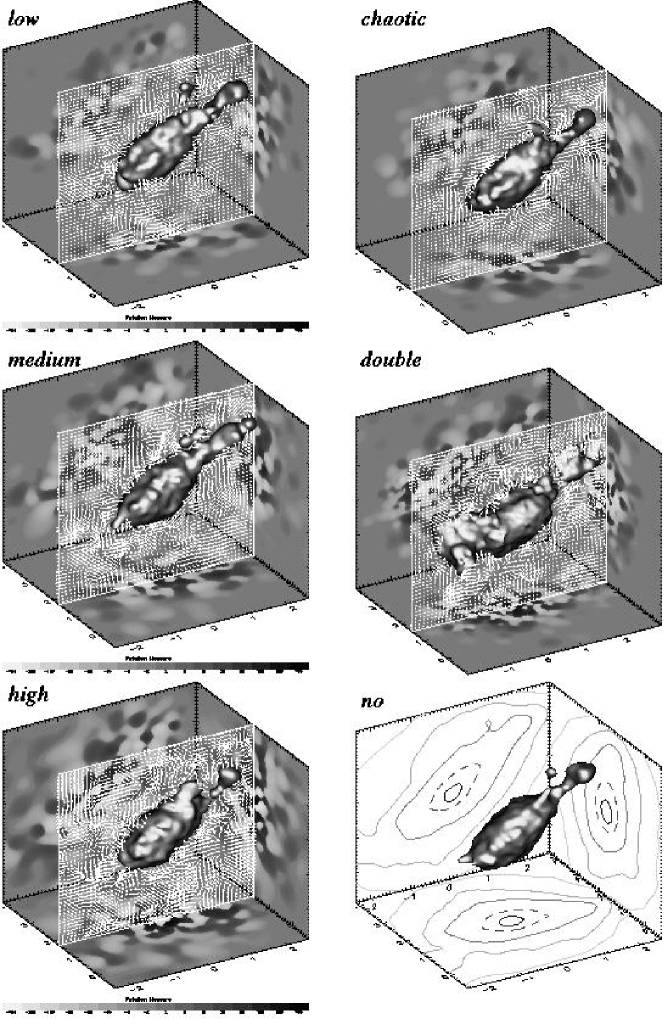
Figure 1: The figure shows versions of the same SCDM galaxy cluster for six different initial magnetic field models as indicated in the plot, including one version without magnetic field for reference. Plotted are the projected rotation measure maps, an iso-density surface and a cut through the magnetic field.

Furthermore, we point out that as we are including the back-reaction of the magnetic field on the gas, different initial field strengths and configurations are changes to the initial conditions from which the clusters develop, hence their evolution proceeds in a somewhat different way. This implies that even a low magnetic field can alter the dynamical time scale of a simulated cluster to some degree. Therefore, when comparing simulated clusters with different initial magnetic fields at equal redshifts, one has to keep in mind that they can be in slightly different evolutionary stages according to their individual dynamical time scale. Of course this has an even more pronounced effect on the models with doubled mass resolution. In this case, it is not the magnetic field but the addition of new particles at intermediate positions which changes the initial conditions and leads to slightly different clusters which evolve in a slightly different fashion. Figure 1 provides a visual impression of the differences between six different simulations of one cluster in a pre-merger phase, starting from the same SCDM cluster initial conditions. The simulations use four different configurations of the initial magnetic field, one run without magnetic field, and one with doubled mass resolution.

SCDM	$r<0.1r_{\mathrm{vir}}$		$r<1.0r_{\mathrm{vir}}$
	A [$\mu G$]	$\alpha$	A [$\mu G$]	$\alpha$
low	$5.9\times 10^{-4}$	2.5	$9.4\times 10^{-4}$	2.2
chaotic	$4.0\times 10^{-4}$	2.6	$8.6\times 10^{-4}$	2.3
double	$2.5\times 10^{-3}$	2.6	$1.0\times 10^{-3}$	2.6
medium	$5.0\times 10^{-3}$	2.1	$6.1\times 10^{-3}$	1.9
high	$3.1\times 10^{-2}$	1.7	$3.6\times 10^{-2}$	1.4
$\Lambda$CDM	$r<0.1r_{\mathrm{vir}}$		$r<1.0r_{\mathrm{vir}}$
	A [$\mu G$]	$\alpha$	A [$\mu G$]	$\alpha$
low	$1.1\times 10^{-4}$	3.0	$3.0\times 10^{-4}$	2.5
medium	$1.1\times 10^{-3}$	2.5	$2.5\times 10^{-3}$	2.0
high	$1.0\times 10^{-2}$	2.1	$1.5\times 10^{-2}$	1.7

Table 3: Parameters (amplitude $A$ and slope $\alpha$) of power laws best fitting the relation between final mean magnetic field strength and mean temperature in the simulated clusters. Numbers for different cosmologies, different magnetic field setups and different radii for the averaging volume are determined. The different slopes fitted to the different models are all consistent within the model uncertainties.

3 Structure of the final magnetic field

As reported earlier (Dolag et al. 1999), the process of cluster formation and the surrounding large scale structure entirely determine the magnetic field properties in the simulated clusters. As shown before, all information contained in the structure of the seed field is completely wiped out in the process of the collapse. This means that the final magnetic field properties obtained reflect our understanding of the formation of galaxy clusters, with the underlying general assumption that the magnetic field in galaxy clusters results from the amplification of weak seed fields.

3.1 Amplification by shear flows

Apart from the compression of the magnetic field frozen into the gas, the magnetic field is also substantially amplified by shear flows as the gas is accreted by the cluster. A necessary condition for this amplification mechanism is that the velocity difference across the boundary layer exceeds the local Alfvén speed, which is proportional to the field strength, so that the condition is more easily satisfied for weaker fields. This means that the relative field amplification becomes smaller as the fields grow. As the shear flows are largely driven by gradients in the dark matter potential, this mechanism is quite independent of pressure support by the magnetic field and therefore reduces the relative amplification much earlier than local equipartition is reached.

model	$\langle l_{\mathrm{final}}\rangle_{\mathrm{core}}^{\mathrm{SCDM}}[\mathrm{kpc}]$	RMS
low B	62.6	9.8
chaotic	60.8	22.0
double	55.5	16.5
medium B	51.3	12.9
high B	46.1	18.2

Table 4: Cols. 2 and 3 show typical field-reversal scales in kpc (physical units) for the magnetic fields and their rms deviation for the clusters in the SCDM model. The values are calculated using all particles in cluster-centric spheres with one tenth of the viral radius, and averaged across the sample of ten clusters per cosmological model.

3.2 Final field strength

Figure 2: The mean magnetic field is shown as function of the mean mass weighted temperature inside the clusters. Here, the ten less massive objects identified in the simulations are included in the analysis. The symbols belong to the “medium” model, the lines represent the power laws fitted to all models for the different magnetic seed fields. Both quantities are calculated within 10 per cent (thin symbols and lines) and 100 per cent (thick symbols and lines) of the virial radius. The left side represents the SCDM models, the right side the LCDM models, respectively.

One quantity of primary theoretical interest is the final magnetic field strength in galaxy clusters predicted by our models. Of course, it depends on the strengths of the seed fields assumed in the simulations. The final magnetic field strengths also depend on the final cluster mass and on the dynamical state of the galaxy cluster because mergers are known to amplify the magnetic field (Roettiger et al. 1999, Dolag et al. 1999).

The simulations also predict that the magnetic field decreases with increasing cluster-centric distance. Therefore, we compute the mean magnetic field strengths within 10 per cent and 100 per cent of the virial radius of the final cluster. Figure 2 shows how the mean magnetic field strength scales with temperature for three sets of initial field strengths in our SCDM simulations. In order to increase the temperature range of our cluster set, we also include ten less massive objects found near the most massive clusters in our simulations. We thus ended up with a total of twenty different objects for every initial magnetic field configuration in both cosmologies.

We fitted this relation in all sets of simulations by a power law, $\langle B\rangle=A\,T^{\alpha}$. The values of $A$ and $\alpha$ we obtained for all our simulations in both cosmologies are summarised in Table 3. In Fig. 2, the different symbols and line types distinguish between the different initial field models. The thin and thick symbols and lines show results calculated within 10 per cent and 100 per cent of the virial radius, respectively.

As Table 3 shows, this relation tends to flatten when the magnetic field strength is averaged within a larger volume, and also when the initial seed magnetic field strength is increased. These trends are not significant given the uncertainties of the models, but they may have the same reason as the flattening of the magnetic field profiles towards the cluster cores, which will be discussed below. It is simply the fact that smaller magnetic fields can more easily be amplified by shear flows than already grown magnetic fields, as discussed before. These relations again show that there is no difference in the final states of the simulation sets with “chaotic and “homogeneous initial field configurations, which confirms that the information on the initial field configuration gets entirely wiped out during the process of cluster collapse. There is also no visible difference between the two cosmologies. Doubling the mass resolution does not significantly change the final field structure either, although the field amplification is higher.

Figure 3: The two panels show the radial profiles of the magnetic field strengths (thick lines) in the simulated, final clusters. The profiles are obtained by averaging across the sample of ten clusters. The averaged gas density profiles, raised to the power of $2/3$, are over-plotted for comparison as the thin lines, arbitrarily normalised to the amplitude of the magnetic-field profiles at the virial radius. The left panel shows the SCDM simulations for the various initial field configurations, as labelled in the plot. The right panel shows the results for the $\Lambda$CDM models.

Another interesting result of the simulations is the relation between the magnetic field strength and the gas density in the clusters. Figure 3 shows the mean magnetic field strength in spherical shells centred on the cluster centre as function of cluster-centric distance in units of the virial radius. Plotted are the profiles at redshift zero, but the shape does not change significantly between redshift one and zero. The gas density profiles, averaged across the sample of ten clusters and raised to the power of $2/3$, are over-plotted in arbitrary units to match the magnetic field strength amplitude at the virial radius (dashed lines).

The average magnetic field strength profiles in the outer regions of the clusters (beyond $\sim 0.3\,r_{\mathrm{vir}}$) follow the density profile very well, while they flatten off towards the cluster core, where the magnetic field profiles are shallower than the density profiles. Plotting the density profile raised to the power of $2/3$ demonstrates that in the outer parts of the cluster, the average magnetic field strength is more strongly amplified as expected from compression alone ($\propto\rho^{2/3}$), thus shear flows have to play an important role there. In the centre, the field amplification is reduced. This is due to the fact that the higher magnetic field strength in the cluster centres slows down the further field amplification compared to the outer cluster regions. There are two reasons for that. First, the motions of the gas are less coordinated in the cluster cores compared to the large-scale motion of the infalling gas in the outer parts, so that amplification by ordered shear flows is suppressed. Moreover, increasingly important back-reaction of the field on the gas flow counteracts further amplification. Second, the magnetic field is also substantially amplified by shear flows as the gas is accreted by the cluster. A necessary condition for such an amplification is that the relative velocity on both sides of the boundary layer exceeds the local Alfvén speed which is proportional to the field strength, so that the condition is more easily satisfied for the weaker fields embedded in the infalling material in the outer regions of the clusters than for the stronger fields near cluster centres.

This is also responsible for flattening the relation between temperature and magnetic field strengths for increasing initial magnetic field strength. Table 2 lists the final magnetic field strengths in the cores of the simulated cluster sample for the different initial magnetic field configurations. Again, the chaotic and the homogeneous initial field configurations lead to the same radial magnetic field strength profiles. As observed before in Dolag et al. (1999), the final magnetic field structure is entirely driven by the collapse of the galaxy cluster, and any information about the initial field structure is completely erased. This justifies the use of homogeneous initial conditions for the magnetic field setup, as they are numerically easier to handle. The profiles do not change significantly when the particle number is doubled.

These results on the radial magnetic field strength profiles and the dependence of mean field strengths on the cluster temperature may help to reconcile the observations in different galaxy clusters, which seem to give somewhat different values for the magnetic field for different clusters observed. In addition, the difference between magnetic field inferred from Faraday rotation measurements on the one hand (testing the line-of-sight average) and the combination of radio emission with hard X-ray observations on the other hand (measuring volume averaged magnetic fields) could be bridged using our simulations, although the relativistic electron density needs to be assumed. Comparing the mean magnetic field within the virial radius and one tenth of the virial radius, the data points in Fig. 2 show that these values differ already by factors of five, or more.

3.3 Field reversals

Figure 4: The figure shows the autocorrelation function of the magnetic field, $\langle\@vec{B}(\@vec{x})\cdot\@vec{B}(\@vec{x}+\@vec{d})\rangle$ as a function of $|\@vec{d}|$ for one SCDM cluster, simulated with five different initial conditions for the magnetic field, as indicated in the plot. The numbers attached to the minima and maxima indicate the number of particle pairs used to compute the mean value. Only particles within ten per cent of the virial radius are taken into account. All curves are normalised to fall within $\pm 1$ within the region shown. Table 4 lists the mean inferred autocorrelation length scale across our cluster sample and its rms deviation.

The formation of large scale structure in the surroundings of a cluster also imprint some structure on the magnetic field of galaxy clusters. Large scale flows can order magnetic fields parallel with the flow. Also the field compression in shock fronts orders the magnetic fields to some degree. Since the shocks compress the medium in only one direction, the magnetic fields in the shocked gas tend to lie within the surface of the shock shell. On the other hand, the more chaotic motion of the gas inside cluster cores tends to destroy the order imposed on the magnetic field during cluster collapse. We thus expect a complicated behaviour of the field structure and a range of autocorrelation length scales. It is of interest for the interpretation of rotation measures on what scales field orientations reverse inside cluster cores. Our simulations predict how magnetic fields can be ordered in the process of large scale structure formation and gravitational collapse. In addition, there might be smaller scale contributions from the outflows and the cocoons of the radio galaxies, from which Faraday rotations are measured.

In order to infer this typical length scale in the simulated clusters, we cut out the central sphere with one tenth of the virial radius of each cluster and calculate the autocorrelation function

$$\xi(\@vec{d})=\langle\@vec{B}(\@vec{x})\cdot\@vec{B}(\@vec{x}+\@vec{d})\rangle$$ (1)

by identifying all possible pairs of particles, sorting them by their separation, and binning them. The mean is then calculated over the number of particles in each distance bin. This function should be positive for scales smaller than that of typical field reversals, then go through a minimum at this typical length scale, and then damp due to the mixing of different length scales. This mixing, the presence of shocks, and the layers between shear flows, already affect this measurement at the length scale of interest, which render the determination (and even the meaning) of the length scale dubious. On larger scales, it gets confused by the mixture of different length scales present in the cluster. Therefore, the minimum correlation length scale is difficult to measure.

Figure 4 shows the autocorrelation function for one simulated SCDM cluster. At small scales, this function shows the positive value expected, but it is already very noisy. Note that the innermost distance bin is narrower than the average inter-particle distance, and are therefore likely to be in shocks.

Although the magnetic field in the shocks is preferentially aligned tangentially to its surface, the orientation within this surface can be very tangled. Accordingly, the innermost bin is very noisy and can even yield negative values, as seen in the “low” model. At somewhat larger distances, the autocorrelation function becomes positive, as expected. Then, at almost twice this distance, $\xi(\@vec{d})$ becomes negative, also as expected. Clearly, the field autocorrelation function is determined by the structure of the cluster and shows a very similar behaviour for different initial magnetic field configurations in that it consistently reaches a pronounced minimum between 60 and 80 kpc. The numbers attached to the individual lines denote the number of particles used to calculate the mean within this distance bin. At the first minimum, several hundred particles are used to compute the SPH average. The autocorrelation function reaches zero only beyond the plotted range.

Figure 5: This figure shows the magnetic field component in the $x$ (solid line) and $y$ directions (dashed line) along a line-of-sight through one of the simulated clusters. This line was chosen parallel to the $x$ axis and passing through the cluster centre. The envelope of the curves follows the general radial decrease in the magnetic field strength. It is clearly seen that field reversals are relatively more frequent in the cluster centre, and relatively less frequent away from the cluster core.

Since the autocorrelation signal is the result of mixing structures with different length scales (due to substructure), regions simulated at varying spatial resolutions (because of the adaptive SPH kernel), and volumes with varying magnetic field strength (due to the field structure in the cluster), it is not at all straightforward to read off a characteristic autocorrelation scale from such plots for all clusters. In order to obtain a more robust estimator, we tried to read off the first two extrema and the zero, and constructed the appropriately weighted mean

$$l=(2\,l_{\mathrm{drop}}+l_{\mathrm{zero}_{1}}+2/3\,l_{\mathrm{min}}+1/2\,l_{\mathrm{zero}_{2}})/4$$ (2)

of the positions of the extrema to get the length scale $l$ rather than trying to identify the location of the first minimum only. Interpreting the signal like a wave and taking the distance between the zero crossing as the length-scale of the magnetic field, $l_{\mathrm{drop}}$ in this equation is the length scale where the signal starts to decrease, which is an indicator of half the typical length of the magnetic field $l_{\mathrm{zero}_{1}}$, where the signal is expected to drop to zero. The next minimum $l_{\mathrm{min}}$ should reflect $2/3$ of the magnetic field reversal scale. We may also get a second minimum, $l_{\mathrm{zero}_{2}}$, reflecting twice the magnetic field reversal scale, before the signal fades out due to the reasons mentioned above.

Table 4 summarises the field reversal scales found in the simulations. The table lists the averages across the sample of ten clusters for each set of simulations and their rms deviations. Clearly, the reversal scale does not depend on the structure and the strength of the initial magnetic field. Doubling the particle resolution does not yield significantly different answers either.

3.4 Field structure

The length scale on which the magnetic field typically reverses its direction is important for the interpretation of Faraday rotation measurements. Since the Faraday rotation measure is an integral of the magnetic field component parallel to the line-of-sight, weighted by the electron density, it is also important to know how the field reversal scale changes across the cluster. Figure 5 shows one line of sight passing through the centre of one of the simulated clusters. The solid and dashed lines show the $x$ component (along the line-of-sight) and $y$ component (perpendicular to the line-of-sight) of the magnetic field along the line-of-sight, respectively. The line-of-sight was chosen to go through the centre of mass of the cluster and follows the $x$ axis. Notice that the plot is composed of four panels, where the regions near zero are cut out to allow a logarithmic scale.

Figure 6: This figure shows the magnetic-field power spectra calculated from the simulation of one galaxy cluster for different initial magnetic field configurations, distinguished by different line types as indicated in the plot. For each simulation, the best-fitting power law is overlaid.

It can be read off the figure how frequently the magnetic field changes it direction, and how the reversal length scale changes with the distance from the cluster centre. The envelope of the curves in this plot nicely follows the radial decline of the magnetic field strength in our simulations. It is also clearly seen that the magnetic field reverses relatively less often in the outer parts of the cluster. While we count $23$ extrema for the $x$ component of the magnetic field within $\pm 4\,\mbox{Mpc}$ (in physical units), there are already 15 extrema within $\pm 1\,\mbox{Mpc}$ (in physical units).

This effective increase in the reversal length scale has to be taken into account equally well as the decrease of the magnetic field strength with radius when inferring magnetic fields from Faraday rotation measurements. These effects tend to reduce the magnetic field strengths inferred from current observations.

In order to improve our understanding of the statistical properties of the field structure, we calculated the power spectra of the magnetic field in the simulated galaxy clusters. To this end, we calculated the auto-correlation function of the field strength within a cube of $10\,\mbox{Mpc}$ comoving side length, centred on the cluster centre, using an equidistant grid of $80^{3}$ cells on which all quantities are calculated by means of the SPH formalism.

model	$a$	$b$	$\langle b\rangle$	RMSb
low	9.9	-2.7	—	—
chaotic	10.6	-2.7	—	—
double	8.5	-3.0	—	—
medium	6.8	-2.7	-2.7	0.2
high	3.5	-2.4	—	—

Table 5: Best-fitting parameters for power laws, $a\,k^{b}$, to the magnetic-field power spectra. The table summarises the values for different initial magnetic field configurations in the SCDM models.

In this type of simulation, the dynamical range of spatial scales is not high enough to fully resolve the correlation function over a satisfactory range of length scales. Nonetheless, we could compute the correlation function and the power spectra over one and a half orders of magnitude in length scale, within which it nicely follows a power law. The hump towards small $k$ values (i.e. large radii) can qualitatively be understood. First, the correlation function rises towards the typical distance between major objects within the simulation, e.g. the cluster and the next major object falling onto it. In addition, the correlation function in a cubical simulation volume is over-predicted for scales approaching half the cube side length (i.e. the Nyquist length) because one particle of each pair is most probably positioned near the cluster centre. On even larger scales, one particle of each pair most likely falls outside the cluster core, and therefore the correlation function drops rapidly. On small scales, the resolution of the cube used, and the resolution of the simulation itself, restrict the calculation of the correlation function and thus also the computation of the power spectra.

Nonetheless, it is possible to calculate the power spectra over a reasonably wide range in wave number, and compare the results for different magnetic field configurations. Figure 6 shows the power spectrum calculated from one of the simulated clusters for different initial magnetic field configurations. The power spectra look quite the same for all models.

The exponents of the best-fitting power laws for one set of simulations range from $-2.3$ to $-3.1$, with a mean of $-2.7$. This value is surprisingly low. For Kolmogorov turbulence, $-5/3$ would be expected. A fully established MHD turbulence would produce $-3/2$, and even in the extreme case of a young, incompletely established MHD turbulence, we would expect $-2$ (cf. Eilek & Henriksen (1984) and references therein).

There are two cases discussed in the literature which result in a smaller power-law slope. First, for a 2-dimensional Navier-Stokes turbulence (Biskamp (1993)), an exponent of $-3$ would be expected. As shear flows play a major role in amplifying the magnetic field, it is very likely that we see our cluster simulations in a state, where the turbulence induced by shear flows evolves into a Kolmogorov turbulence. The second case, which leads to a power-law index of $-4$ (Eilek & Henriksen (1984)), is turbulence in a very viscous medium. SPH is known to be viscous, so this may be a possibility to explain the small exponent found, but as the artificial viscosity in SPH is constructed to vanish in shear flows, this is unlikely to be the complete explanation. To clarify this issue, detailed tests remain to be done. Table 5 summarises the power-law fits to the power spectra in the different models. In particular, the spectra for the chaotic and the equivalent homogeneous initial field configurations are indistinguishable. Also, the power spectra for the run with doubled mass resolution do not differ, which argues against a dominant impact of the SPH viscosity on the behaviour of the magnetic field in the simulations. There is also no visible change in the power laws with changes in the magnetic field strength.

Figure 7: The mean magnetic field in one cluster simulated in the SCDM cosmology ($h=0.5$) of those gas particles which at the end of the simulation populate spheres of ten and fifty per cent of the virial radius (dotted and dashed lines) around the cluster centre is shown as a function of redshift. The solid line is the mean magnetic field within a sphere of comoving radius 1 Mpc which remains centred on the most massive cluster component.

4 Magnetic field evolution

This section describes how the magnetic fields evolve during the formation of galaxy clusters in our simulations. The field evolution is driven by structure formation; in particular, major mergers have a strong influence on the how the field evolves.

4.1 Magnetic field evolution

We follow two different approaches for describing the evolution of the magnetic field in our simulations. First, we look at each individual given cluster and measure how the magnetic field strength in the cluster (e.g. within the core) evolves with time. On the other hand, we can ask how the magnetic field evolves which is carried by the gas that finally ends up in the cluster core. The first approach could be considered as Eulerian, the second as Lagrangian.

Figure 7 shows the results of both approaches for one cluster simulated in the SCDM cosmology ($h=0.5)$). The solid line shows the mean magnetic field within a sphere of 1 Mpc radius around the cluster centre. More precisely, it shows the mean magnetic field within a sphere of 1 Mpc comoving radius, centred on the most massive halo contributing to the final cluster. The dotted and dashed lines show as functions of time the mean magnetic fields carried by all particles which finally fall into spheres around the cluster centre with radii of ten and fifty per cent of the virial radius. It is clearly seen that the magnetic field in the core of the evolving galaxy cluster is stronger than the magnetic field in the cluster surroundings, which are finally accreted by the galaxy cluster. All three curves show pronounced maxima which coincide with major mergers at redshifts $0.5$ and $0.2$, and likewise at the second core passage of a major merger at redshift $0.7$. Also, the combined effect of a second core passage and a merger at redshift $\sim 0.2$ can be seen here, and more explicitly in Fig. 8. The magnetic field in the cluster cores and in related shocks during mergers is increased substantially. Even the mean field within a large volume can be increased by a factor of a few, as can be read off Fig. 7.

SCDM	$5$	$20$	$50$
low B	$-0.23$	$-0.33$	$-0.31$
medium B	$-0.09$	$-0.15$	$-0.15$
high B	$-0.04$	$-0.07$	$-0.08$
$\Lambda$CDM	$5$	$20$	$50$
low B	$-0.29$	$-0.34$	$-0.42$
medium B	$-0.16$	$-0.18$	$-0.24$
high B	$-0.09$	$-0.11$	$-0.15$

Table 6: This table summarises the slopes of the linear fits shown in Fig. 9 for different cosmologies and different Faraday-rotation thresholds.

4.2 Influence of mergers on observables

We now investigate how the projected patterns of Faraday rotation measures evolves. In doing so, we calculated synthetic rotation measure maps for 60 epochs between redshifts $0.8$ and $0$ (today). For each epoch, we have one map for each of the three different projection directions (chosen to be the coordinate axes). In each map, we calculate the total area of those regions in which the rotation measure exceeds a given threshold (in other words, we compute the measure of the excursion set of the Faraday rotation).

Figure 8 shows this area as a function of time (or redshift), normalised to the area which emits 95% of the X-ray luminosity. The different line types distinguish between the three different projection directions, the three bundles of lines are for rotation measure thresholds of 5, 20, and 50 rad/m². The general tendency for this quantity to grow with time is evident, as is expected from the growing magnetic field. The structure seen in the time evolution is clearly related to merger events. All peaks on these curves correspond to a core passage during a merger event. Likewise, the second core passage after the merger causes the area to peak. The signal does not strongly depend on the projection direction, and the sequence of peaks is present for all rotation-measure thresholds chosen. This provides clear evidence that merger events strongly contribute to the amplification of the magnetic field, an effect which is confirmed by other simulations (Roettiger et al. 1999). Since this effect is visible in all projections, this also applies to mergers along the line-of-sight, whose X-ray contours look quite regular. This implies that determining the area covered by Faraday rotation measures above a fixed threshold may help constraining cluster mergers in such configurations.

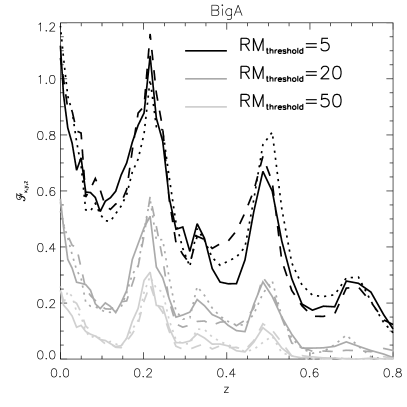
Figure 8: This figure shows how the area, covered by a Faraday rotation measure exceeding thresholds of 5 (upper bundle), 20 (middle bundle) and 50 rad/m² (lower bundle) evolves with time. The area is normalised by the area emitting 95% of the cluster X-ray luminosity. The different line types distinguish the three different projection directions.

4.3 Evolution in different cosmologies

Figure 9 shows the same area, but averaged over all ten realizations. The sequence of peaks is smoothed out, leaving the general trend. The different initial field configurations are indicated by different types of symbol, as indicated in the plot. We overlay fits showing that the growth is very well fit by linear functions. Table 6 summarises the gradient inferred from these fits for different cosmologies, different initial field configurations and different thresholds.

Figure 9: This figure shows the same quantity as shown in Fig. 8, but only for the one threshold of 20 rad/m², and averaged over the three projection directions and over the ten clusters per sample. The different line types represent the different sets of models for the initial magnetic field. The left panel shows results for the SCDM cosmology, the right panel for the $\Lambda$CDM cosmology.

5 Comparison with measurements

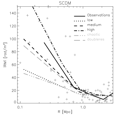
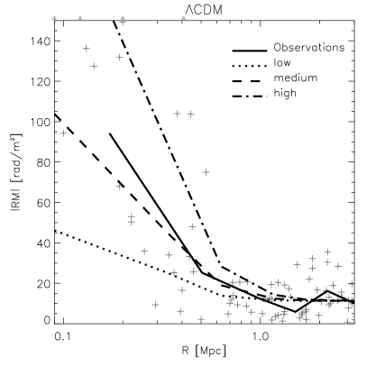
Figure 10: This figure shows a comparison of observed Faraday rotation measures with our simulations. Plotted is the absolute value of the observed rotation measures as a function of the distance to the next Abell cluster (crosses), taken from Clarke et al. (2001). The solid line marks the sample median of the observations. The superposed lines are calculated from synthetic Faraday rotation measurements taken from our simulations in an attempt to mimic the observations. The different line types distinguish between the different initial magnetic field configurations used in the simulations. The left and right panels show SCDM and $\Lambda$CDM results, respectively. The Medians were calculated in bins containing 15 data points each. The shape of the synthetic measurements in both cosmologies follow very well the observations. To perfectly match the observations in this comparison, a magnetic field somewhere in between the “medium” and the “high” models is needed.

Figure 10 compares the measurements of Clarke et al. (2001) with the synthetic Faraday rotation measures taken from our simulations. These new measurements are in excellent agreement with previous measurements collected by Kim et al. (1990), and are also compatible with Faraday-rotation measurements in individual clusters like Abell 119 by Feretti et al. (1999).

To calculate the synthetic signal, we computed three rotation-measure maps for the three spatial projects for each cluster on a grid of $60^{2}$ cells, covering $5\times 5\,$Mpc (physical units). For each cosmology and all initial magnetic field configurations, the Faraday-rotation measures are sorted in radial bins and combined over all ten realizations. The simulated values compare very well with the observations. We calculated the signal from the observations between 3 Mpc and 10 Mpc as a reference (11 rad/m²) and added this as a background to the synthetic data. The synthetic curves very well follow the shape of the measurement distributions. It is also easily seen that the initial magnetic field strength required to reproduce the observations falls somewhere between the “medium” and the “high” models.

Again, it is obvious that the difference for the two different initial field configurations, namely homogeneous and chaotic, is negligible. Also, the two different resolutions lead to statistically the same signal, but as the mass resolution is only changed by a factor of two, this does not resemble a convergence study.

6 Summary and conclusions

We performed cosmological, magneto-hydrodynamic simulations of galaxy clusters to study the evolution and final structure of magnetic fields frozen into the intracluster medium. In total, we investigated 100 cluster models of different masses in two different cosmologies (standard and open CDM), varying the structure and the strength of the initial magnetic field configuration. Our results can be summarised as follows:

• Starting with magnetic fields of order $10^{-9}\,\mathrm{G}$ at an initial redshift of $z_{\mathrm{ini}}=15$ (20 for $\Lambda$CDM), final fields reach micro-Gauss strength in cluster cores at redshift $z=0$. This amplification factor of $\sim 10^{3}$ was found and discussed earlier (Dolag et al. 1999). It exceeds the amplification factor expected from spherical collapse by an order of magnitude, which can be traced back to field amplification in shear flows.

• Radial profiles of the magnetic field strength closely follow the cluster density profiles at radii of $\sim 200h^{-1}\,\mathrm{kpc}$ and beyond. At smaller radii, the magnetic field strength profiles flatten. This reflects the behaviour of the gas distribution, which also develops a flat core despite the dark-matter density cusp because of the finite gas pressure. In a purely spherical collapse, the magnetic field strength is expected to scale with density raised to the $2/3$ power, flattening the profile. Additionally, the amplification by shear flows works more efficiently when the field strengths are small and therefore the fields get more relative amplification in the outer parts, leading to further flattening of the magnetic field profile compared to the gas profile. This happens independently of the strength and the structure of the initial magnetic seed field, and for both cosmologies investigated.

• The correlation lengths of the magnetic fields in cluster cores are of order $\sim 50h^{-1}\,\mathrm{kpc}$. Similarly, the length scale of field reversals along lines-of-sight through cluster cores is of order $\sim 100h^{-1}\,\mathrm{kpc}$. These length scales show no significant dependence on the initial field strength or configuration, or on cosmology.

• The power spectrum of the magnetic field can closely be approximated by a power law, $P_{\mathrm{B}}(k)\propto k^{-n}$, with a power-law exponent of $n\sim-2.7$. This is steeper than expected for Kolmogorov or MHD turbulence, but close to the expectation for two-dimensional Navier-Stokes turbulence. A possible explanation is the occurrence of essentially two-dimensional shear flows and their importance for the magnetic field evolution in clusters. Although we do not expect this to be a strong effect, the high numerical viscosity in SPH codes also tends to steepen the power spectrum.

• Predominantly driven by merger events, the mean magnetic field in cluster cores grows roughly exponentially with redshift. Between redshifts $z=0.8$ and $z=0$, the growth is well approximated by

  $$|\@vec{B}|(z)\approx 10^{-2.5\,z}\,\mu\mathrm{G}\;.$$ (3)

  Superposed on this general trend is the effect of mergers, during which the magnetic field strength goes through pronounced maxima.

• Field amplification by mergers shows up prominently in observable quantities like the Faraday rotation. During mergers, the projected cluster area in which substantial Faraday rotation occurs rises sharply, and it drops during the subsequent relaxation phases.

• Simulated Faraday rotation measures show that all our cluster models are in excellent agreement with the largest available sample of observed Faraday-rotation measurements, although the samples are still too small to provide narrow constraints on, e.g., the initial strength of the magnetic seed fields.

Our results therefore show that the strength of intracluster magnetic fields grows rapidly with redshift, and it closely follows the cluster density profiles outside a core region of $\sim 200h^{-1}\,\mathrm{kpc}$ radius. The structure of the field can be characterised by an auto-correlation or reversal scale of order $50-100h^{-1}\,\mathrm{kpc}$, well above the spatial resolution of our numerical simulations. The power spectrum of the magnetic field falls steeply, but the distribution of energy density with respect to $k$ scales as $k^{3}\,P(k)$ and thus remains monotonically increasing. This indicates that most of the magnetic energy density is located on small scales.

The independence of these results on cosmology and initial field structure demonstrates that the final intracluster fields are entirely dominated by the cluster collapse, thus confirming and extending the previous findings (Dolag et al. 1999). The importance of mergers for observable signatures of intracluster magnetic fields, and their steep evolution with redshift, suggest important observational tests for the scenario underlying the formation and evolution of our simulated galaxy clusters.

References

- Bartelmann & Steinmetz (1996) Bartelmann, M. & Steinmetz, M., 1996, MNRAS, 283, 431-446
- Biskamp (1993) Biskamp, D., 1993, “Nonlinear Magnetohydrodynamics” (Cambridge University Press 1993, ISBN 0 521 40206 9)
- Brio & Wu (1988) Brio, M. & Wu, C.C., 1988, J. Comput. Phys., 75, 400
- Clarke et al. (2001) Clarke, T.E., Kronberg, P.P. & Böhringer H., 2001, ApJ 547, L111
- Dolag et al. (1999) Dolag, K., Bartelmann & M., Lesch, H., 1999, A&A, 348, 351
- Eilek & Henriksen (1984) Eilek, J.A. & Henriksen, R.N., 1984, ApJ, 277, 820
- Eke et al. (1998) Eke, V.R., Navarro, J.F. & Frenk, C.S. 1998, ApJ, 503, 569
- (8) Ferretti, L., Dallacasa, D., Govoni et al., 1999, A&A, 344, 472
- Kim et al. (1999) Kim, K.T., Kronberg, P.P. & Tribble, P.C., 1991, ApJ, 379, 80
- Kim et al. (1991) Kim, K.T., Kronberg, P.P. & Tribble, P.C., 1991, ApJ, 379, 80
- Lucy (1977) Lucy, L., 1977, AJ, 82, 1013
- Monaghan (1992) Monaghan, J.J., 1992, ARA&A, 30, 543
- Roettiger et al. (1999) Roettiger, K., Stone, J.M. & Burns, J.O., 1999, ApJ, 518, 594
- Steinmetz (1996) Steinmetz, M., 1996, MNRAS, 278, 1005
- Sugimoto et al. (1990) Sugimoto, D., Chikada, Y., Makino, J. et al., 1990, Nature, 345, 33