Spectral Components of the Radio Composite Supernova Remnant G11.2$-$0.3

Abstract

We present a high-resolution radio study of the supernova remnant (SNR) G11.2$-$0.3 using archival VLA data. Spectral tomography is performed to determine the properties of this composite-type SNR’s individual components, which have only recently been distinguished through X-ray observations. Our results indicate that the spectral index of the pulsar wind nebula (PWN), or plerion, is $\alpha_{P}=0.25^{+0.05}_{-0.10}$. We observe a spectral index of $\alpha_{S}=0.56\pm 0.02$ throughout most of the SNR shell region, but also detect a gradient in $\alpha$ in the south-eastern component. We compare the spectral index and flux density with recent single-dish radio data of the source. Also, the radio efficiency and morphological properties of this PWN are found to be consistent with results for other known PWN systems.

1 INTRODUCTION

The proposed association between G11.2$-$0.3 and the supernova (SN) event of 386 ad (Clark & Stephenson, 1977) has prompted many years of detailed study of this object. Radio and X-ray observations made with the Very Large Array (VLA) and Einstein satellite by Downes (1984) verified the existence of a highly symmetric shell. Downes then argued that G11.2$-$0.3 was likely the result of either a 300-500 yr old Type I SN explosion like Tycho or Kepler’s supernova remnant (SNR), or an explosion similar to the event which produced SNR Cassiopeia A, but which took place in 386 ad. Morsi & Reich (1987) detected possible flat spectrum emission in the central region from high-frequency radio maps made with the Effelsberg 100-m telescope, and concluded that G11.2$-$0.3 belongs to a plerion-shell composite SNR class. Overall spectral index estimates of $\alpha=0.56$ (Downes, 1984) and $\alpha=0.49$ (Morsi & Reich, 1987), where $S_{\nu}\propto\nu^{-\alpha}$, were determined from old and recent integrated flux density measurements. Further VLA observations (Green et al., 1988) produced high resolution maps at 20 and 6 cm, and revealed clumpy emission at the outer shell boundry, giving it the appearance of an evolved Type II SNR similar to Cas A. Green et al. (1988) also estimated a distance of $\sim 5$ kpc to the remnant based on its H I spectrum, and a diameter of $\sim 6$ pc. Reynolds et al. (1994) further supported the hypothesis linking G11.2$-$0.3 to the historical event through correlations between radio and ROSAT X-ray observations, but argued for a Type Ia progenitor SN.

Hard-spectrum, non-thermal X-ray emission from a source within the remnant was detected in data from ASCA, which implied the existence of an embedded pulsar producing plerionic emission (Vasisht et al., 1996), and confirmed that G11.2$-$0.3 is a composite remnant. A 65-ms X-ray pulsar (PSR J1811$-$1925) was discovered by Torii et al. (1997); subsequent observations showed the characteristic spin-down age and rate of rotational kinetic energy loss to be $\tau=24,000$ yr and $\dot{E}=6.4\times 10^{36}$ erg/s, respectively (Torii et al., 1999). The exact location of pulsar PSR J1811$-$1925 and the X-ray morphology of the pulsar wind nebula (PWN) were revealed for the first time in Chandra X-ray images (Kaspi et al., 2001).

Recent high-frequency radio observations using the single-dish Effelsberg telescope revealed the spectral index of G11.2$-$0.3 to be $\alpha=0.50$ for the combined spectrum of the PWN and SNR (Kothes & Reich, 2001). A spectral index of $\alpha=0.57$ for the shell emission alone was also calculated, by subtracting an estimated flat spectrum plerionic component.

Because G11.2$-$0.3 has long been mis-classified as a purely shell radio SNR, here we re-examine this source in light of its composite nature, as recently revealed by hard X-ray observations. In this paper, we re-analyse archival VLA data of G11.2$-$0.3 to determine its spectral index, using the technique of spectral tomography, which is a method that allows us to determine $\alpha$ for both the shell and plerionic regions separately. We compare the flux density and spectral parameters of each feature with results from single-dish radio studies. We also measure the structure and radio efficiency of the PWN to verify that they are consistant with other known plerionic remnants. These results will also be included in interpreting X-ray data results (Roberts et al., in preparation).

2 OBSERVATIONS AND RESULTS

Radio observations of G11.2$-$0.3 were made with the VLA at 20 and 6 cm (L- and C-bands, respectively), between 1984 April and 1985 May. Details of these observations are summarized in Table 1.

Table 1: VLA observational parameters for G11.2$-$0.3

Observing	Array	Frequencies	Bandwidth	Time on Source
Date	Configuration	(MHz)	(MHz)	(min)
1984 Apr 26	C	1465, 1515	50.00	39.5
1984 Jun 06	C	1465, 1635	50.00	18
1984 Jun 06	C	4535, 4965	50.00	19
1984 Jul 05	DnC	1446, 1496	12.50	55.5
1984 Jul 05	DnC	4923, 4873	25.00	144
1984 Aug 27	D	4535, 4965	50.00	14.5
1984 Sep 09	D	4835, 4885	50.00	34.5
1985 Feb 22	A	1415, 1490	6.25	77
1985 Feb 25	A	1415, 1490	6.25	82.2
1985 May 19	B	1415, 1490	6.25	62.3
1985 May 19	B	4640, 4670	6.25	129
1985 May 25	B	1415, 1490	6.25	63.3
1985 May 25	B	4640, 4670	6.25	112.8

Data reduction and analysis were performed using standard procedures within the miriad package (Sault & Killeen, 1999). The data were flux-density and antenna-gain calibrated using the primary calibrator 3C286 (J2000 1331+305). The secondary calibrators 1749+096, 1748$-$253 and 1741$-$038 (B1950) were chosen for phase calibrations, based on observation coordinates and wavelength band. To aid in the process of detection and removal of bad visibilities, we performed calibrations on each data set individually. The header files were adjusted to match pointing centers; this step was necessary to prompt miriad’s restoring process into maintaining the smallest possible synthesized beam.

Combined images at both 20 and 6 cm were formed using multi-frequency synthesis and a uniform weighting scheme. The images were deconvolved using a maximum entropy algorithm (Narayan & Nityananda, 1986). We applied iterative phase self-calibration procedures in multi-frequency mode to make additional corrections to the antenna gains as a function of time. The resulting cleaned maps, as displayed in Figure 1, were convolved with a Gaussian restoring beam of dimensions $2\farcs 6\times 1\farcs 8$ and $2\farcs 1\times 1\farcs 5$ for 20 and 6 cm, respectively.

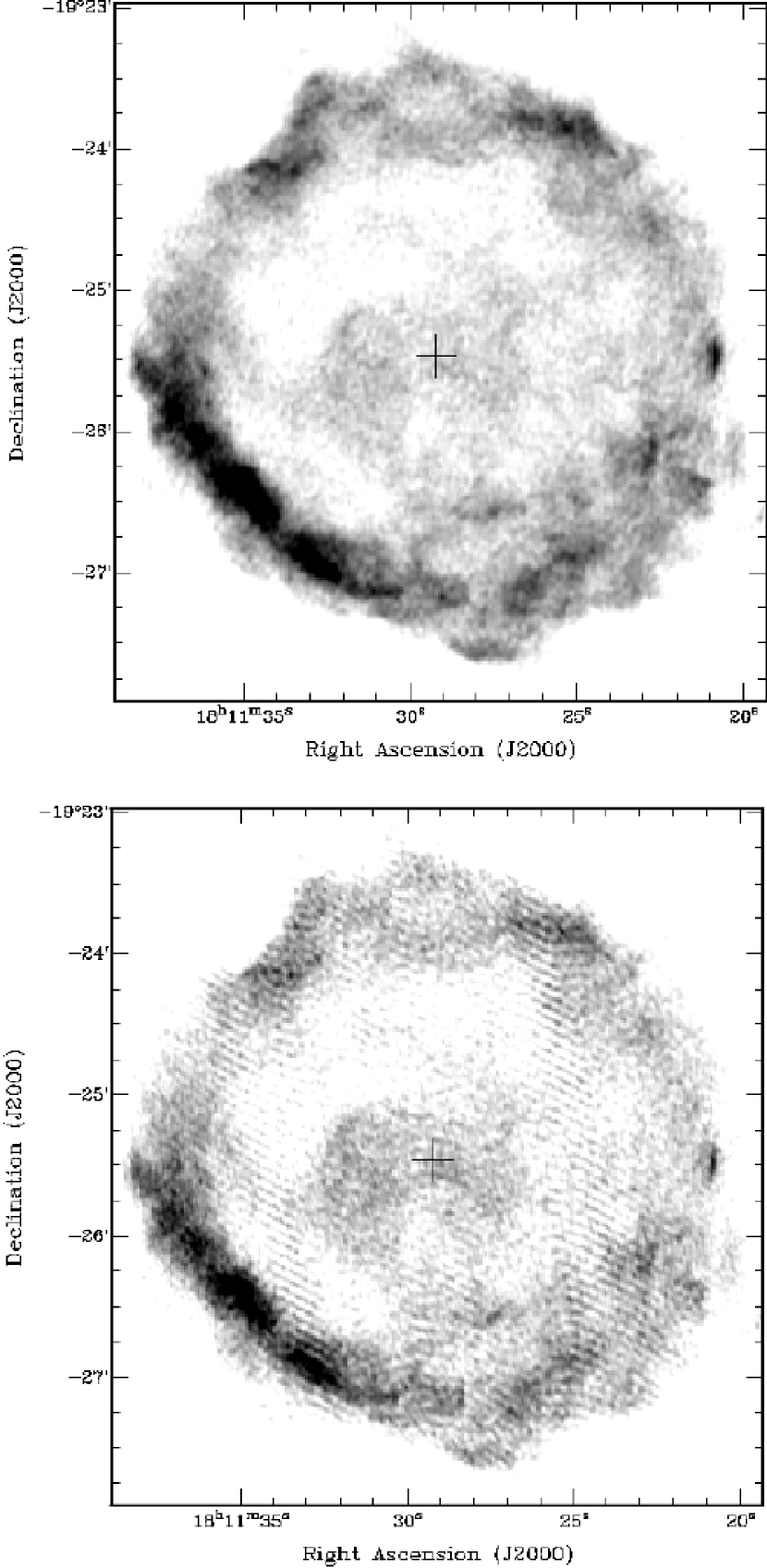
Figure 1: High resolution images of SNR G11.2$-$0.3 at 20 (top) and 6 (bottom) cm. The cross indicates the location of its associated pulsar PSR J1811$-$1925. Note that the size of the cross is much larger than the positional uncertainty (Kaspi et al., 2001). The “stripes” in the 6-cm image are an artifact of emission from a bright point source located to the south (not shown).

2.1 Spectral Index Determination

To measure the spectral index $\alpha$, where $S_{\nu}\propto\nu^{-\alpha}$, from the 20- and 6-cm images, we first needed to spatially filter their $u-v$ sky distributions in order to match spatial scales (Gaensler et al., 1999; Crawford et al., 2001). We degraded the nearly-complete $u-v$ coverage of the 20-cm image to that at 6 cm through a process of $u-v$ modelling, which essentially created a 20-cm visibility dataset with the same coverage as for the 6-cm image. This was imaged and deconvolved in the same way as were the original 6-cm data, and both maps were convolved to 10^′′ resolution to aid clarity in the following tomography process.

We could then compare the two images in order to make a spectral index determination using the method of spectral tomography (Katz-Stone & Rudnick, 1997). A difference image $I_{\alpha_{t}}$ was calculated by scaling the 6-cm image by a trial spectral index $\alpha_{t}$, and subtracting it from the 20-cm image, according to the formula

$$I_{\alpha_{t}}=I_{20}-\left(\frac{\nu_{20}}{\nu_{6}}\right)^{\alpha_{t}}I_{6}\ ,$$

where $I_{20}$ and $I_{6}$ were the images being compared, and $\nu_{20}$ and $\nu_{6}$ were the average frequencies of the combined 20- and 6-cm images, respectively. When the trial spectral index reached the actual spectral index of a particular feature, i.e. $\alpha_{t}=\alpha$, that region appeared to vanish into the local background of the difference image. Uncertainties in $\alpha$ were estimated by finding the range of $\alpha_{t}$ beyond which significant residuals appeared. If a certain area of the feature possessed a slightly different spectral index, it appeared as a distinctly positive or negative residual compared to the rest of the difference image.

2.2 Tomography Results

By examining the series of difference images, we find approximate values of $\alpha$ for the PWN and SNR regions of G11.2$-$0.3. Positive residuals appear as light emission against the neutral grey background, and negative as dark emission.

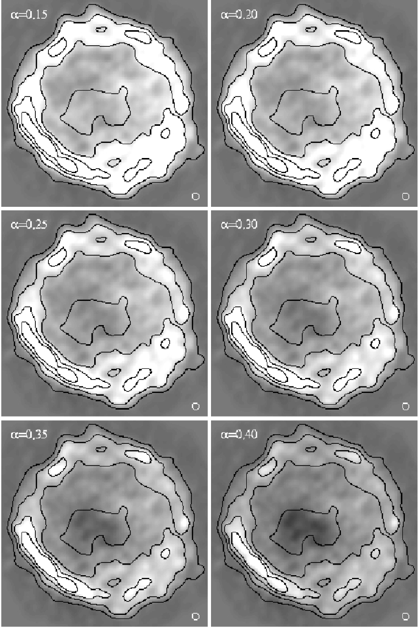
Figure 2: Tomographic spectral index images of the PWN region of G11.2$-$0.3. The greyscale shows difference images for $\alpha_{t}=0.15$ to $0.40$ in steps of 0.05. Contours correspond to 6-cm data convolved with a 10^′′ circular beam (shown in lower right corners), at levels of 5% to 41% of peak flux 91 mJy/beam, in steps of 12%.

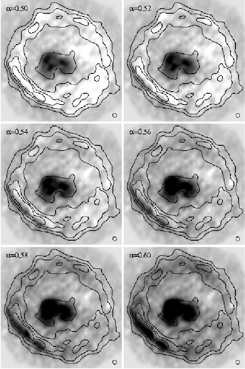
Figure 3: Tomographic spectral index images of the SNR shell region of G11.2$-$0.3. The greyscale shows difference images for $\alpha_{t}=0.50$ to $0.60$ in steps of 0.02. Contours correspond to 6-cm data convolved with a 10^′′ circular beam (shown in lower right corners), at levels of 5% to 41% of peak flux 91 mJy/beam, in steps of 12%.

Figure 2 shows a series of tomographic images between $0.15<\alpha_{t}<0.40$ in $\Delta\alpha=0.05$ intervals. The PWN region in the center disappears into the surrounding region within the shell when the trial spectral index is between $\alpha_{t}\approx$ 0.20 and 0.30. Variations in the appearance of the shell interior between one image and the next suggest that the rms noise here roughly corresponds to a spectral index difference of $\sim 0.05$, although we observe a very clear departure from uniform emission between 0.15 and 0.30; consequently, we choose asymmetric uncertainties around our best estimate of $\alpha_{P}=0.25^{+0.05}_{-0.10}$.

In Figure 3, we show tomographic images between $0.50<\alpha_{t}<0.60$ in $\Delta\alpha=0.02$ intervals. The majority of the SNR shell fades into the surrounding background between $\alpha_{t}\approx 0.54$ and $0.58$; we therefore estimate a value of $\alpha_{S}=0.56\pm 0.02$ for most of the shell region. However, it appears that the SNR spectral index is not completely uniform, most noticeably in the southeastern region. At $\alpha_{t}=0.52$, dark patches can be seen in the outer shell; likewise, lingering positive residuals appear as lighter emission in the inner shell of the same region at $\alpha_{t}=0.58$. This gradient indicates that the spectrum for the outer shell is slightly flatter, and the inner shell slightly steeper, than for the bulk of the remnant. However, it should be noted that the similar size of the 6-cm beam relative to G11.2$-$0.3 may have produced this apparent gradient if the primary beam is not perfectly modeled. Mosaiced VLA observations are currently underway which will verify this feature.

Our measured values for $\alpha_{P}$ and $\alpha_{S}$ are in agreement with single-dish data as published by Kothes & Reich (2001), who predict a fitted spectral index of $\alpha_{total}=0.50\pm 0.02$ from integrated flux density values of the total remnant. Assuming a flat spectrum core of $\alpha_{P}=0$, they subtracted the pulsar wind component of the emission from the total, and inferred $\alpha_{S}=0.57$. This value is well within the uncertainty of our result. They also discuss shell structure, specifically, the southeastern region’s appearance of being in a later evolutionary phase than the rest of the SNR, based on polarization properties and X-ray observations. The possibility of a connection between their conclusion and our detected gradient in $\alpha$ should perhaps be investigated further.

2.3 Flux Density

Using miriad, we determined the integrated flux over various regions in the source, and subtracted the background signal estimated from nearby sky. We estimate the background-subtracted flux density of the entire source to be $S_{T}=16.6\pm 0.9$ Jy at 20 cm and $8.4\pm 0.9$ Jy at 6 cm. Similarly, we subtract the background interior to the shell surrounding the plerionic region to find the PWN flux density $S_{P}=0.36\pm 0.23$ Jy (20 cm) and $0.32\pm 0.18$ Jy (6 cm). The uncertainties are inferred from the rms variations of flux in the background; however, while the exterior background was relatively uniform in brightness, the interior background was highly irregular, causing the large uncertainties in the PWN flux. We then estimate the SNR shell flux density to be $S_{S}=16.2\pm 1.1$ Jy (20 cm) and $8.0\pm 1.1$ Jy (6 cm) based on these measured results.

The greatest source of systematic uncertainty in these values is a result of flux missing due to the nature of interferometric measurements having incomplete $u-v$ coverage. Single-dish measurements would not be subject to the same uncertainty; consequently, in comparing our results with those of Kothes & Reich (2001), we estimate that $\sim 5$% of the total 20-cm flux and $\sim 12$% of 6-cm total flux is missing from our maps. We also measure the amount of missing 6-cm emission resulting from incomplete coverage by comparing the flux levels found in the 20-cm image before and after the $u-v$ modelling process. This $\sim 11$% difference in the total object and $\sim 13$% difference in the plerion indicates how much flux is lost in the 20-cm data by degrading it to 6-cm visibility, thereby implying that the 6-cm data are also missing $\sim 11$%$-13$% flux.

3 DISCUSSION

3.1 Spectral Properties

Table 2: Integrated flux density measurements of G11.2$-$0.3

Frequency	Flux Density	Reference
(MHz)	(Jy)
330	39.0 $\pm$ 2.0	Kassim (1992)
408	34.8 $\pm$ 2.4	Kassim (1989); Shaver & Goss (1970)
1408	17.7 $\pm$ 0.7	Reich, Reich & Fuerst (1990)
2695	11.5 $\pm$ 0.5	Reich et al. (1984)
4850	9.6 $\pm$ 0.5	Kothes & Reich (2001)
10450	6.3 $\pm$ 0.4	Kothes & Reich (2001)
14700	5.7 $\pm$ 0.4	Kothes & Reich (2001)
23000	4.7 $\pm$ 0.5	Kothes & Reich (2001)
32000	3.8 $\pm$ 0.4	Kothes & Reich (2001)

We now compare the results of past studies (see Table 2) with our measurements of spectral index and flux density at 20 cm. To do this, we plot an integrated fitted spectrum of the form

$$S_{T}=S_{S}(\nu/1461)^{-\alpha_{S}}+S_{P}(\nu/1461)^{-\alpha_{P}}\ ,$$ (1)

where $\nu$ is the frequency in MHz. Because of uncertainties in background subtraction and incomplete $u-v$ coverage, we choose to plot an upper and a lower estimate for each value of flux density. We set $S_{P}=0.36\pm 0.23$ as our low value estimate, because we used a region of high flux as background (i.e. inside the shell), and also because of missing interferometric flux. By assuming the lowest possible background (i.e. outside the shell), we find a high value for $S_{P}$, which gives a low limit estimate for $S_{S}$ of $15.4\pm 0.9$ Jy. In order to account for possible missing interferometric flux, we deduce high flux estimates by subtracting our lower bounded values from interpolated total power results of Kothes & Reich (2001). The high estimates for $S_{S}$ and $S_{P}$ are approximately $17.0\pm 0.9$ Jy and $2.0\pm 1.6$ Jy, respectively. Figure 4 shows Equation 1 plotted with our best high and low estimates of $S$, and maximum and minimum uncertainties of $\alpha$. We find our values to be consistent with single-dish values, within estimated uncertainties. The higher frequency data points suggest that the true value of $S_{P}$ may be close to our upper estimate; we therefore assume $S_{P}\sim 1$ Jy for our rough calculations of radio efficiency.

Figure 4: Log-log plot of G11.2$-$0.3 flux density spectrum. See Table 2 for flux data points. The fits correspond to the power-law spectrum (Eq. 1), with the upper and lower bound parameters for $S_{S},\ S_{P},\ \alpha_{S}$, and $\alpha_{P}$, respectively, as listed in the legend. A detailed description of the upper and lower limits is found in § 3.1.

3.2 Morphology and Age

The tomography difference images allow us to identify each feature according to its spectral index. In particular, we recognize the region of central emission that belongs to the PWN as outlined in the $\alpha_{S}$ difference maps (Fig. 3) by the prominent area of dark emission. A contour of this region is projected onto a detailed map of the plerionic region of G11.2$-$0.3 in Figure 5. In this image, it is apparent that the protruding feature in the northwestern direction, and possibly a smaller, similar feature in the southeastern direction, is not spectrally part of the PWN, but may still be associated with emission from the interior of the remnant. A toroidal/jet morphology has been detected in the Crab PWN, so it is possible that we may also be seeing a similar shape here. If it is a torus, then it is most likely centered very near the pulsar position, with an axis of $\sim 30\arcdeg$ west of north. There is some unexplained emission south of its eastern branch, which appears to be associated with the PWN but does not fit into the toroidal morphology, in addition to the protrusions to the NW and SE, which are unassociated with the PWN. Further discussion on the plerionic structure will be presented by Roberts et al. (in preparation), as will the relationship between hard X-ray and radio emission.

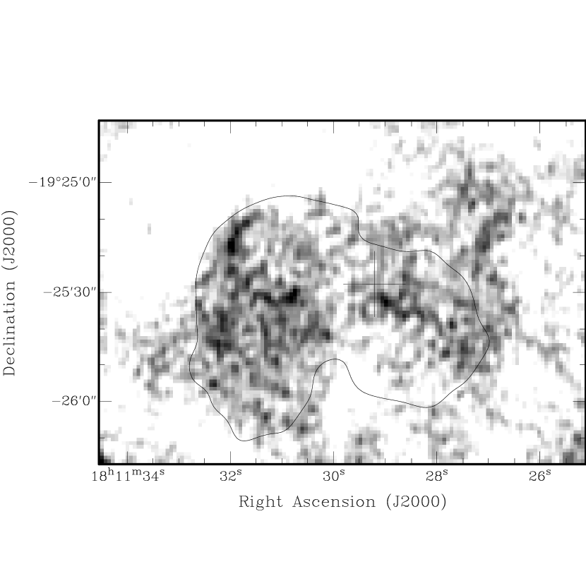
Figure 5: Image of the PWN region in G11.2$-$0.3 at 20 cm. The contour represents roughly the PWN region boundary, as indicated by the spectral tomography difference images. The cross indicates the location of the pulsar, as in Figure 1.

We measure the angular diameter of the SNR to be $\sim 4\farcm 5$ at maximum extent, which corresponds to a linear diameter of $D_{S}\sim 6.5$ pc, assuming the distance $d\sim 5$ kpc to the remnant is accurate (Green et al., 1988). To calculate the average diameter of the PWN, we find the total area encompassed by the plerion and approximate it as radially symmetric, resulting in an angular diameter of $\sim 1\farcm 3$ and $D_{P}\sim 1.8$ pc. The Chandra X-ray image shows a PWN diameter of nearly $1\farcm 3$ (Kaspi et al., 2001), consistent with radio results. The ratio of diameters is $\sim 0.28$ in radio; we compare this value against results for other composite remants and find it to be higher than most other reported ratios (van der Swaluw & Wu, 2001). Current theory predicts two main phases of PWN evolution inside the shell. In the first phase, a bubble of plerionic gas freely expands into the supernova ejecta supersonically, until it encounters the reverse shock of the SNR blast wave, which compresses the plerion. In the second phase, the PWN continues to expand within the SNR at subsonic velocities, as described by a Sedov solution (Reynolds & Chevalier, 1984; van der Swaluw & Wu, 2001). Results of hydrodynamical numerical simulations predict the largest radial extent ratio at the point just before the reverse shock has reached the PWN (Fig. 8 of van der Swaluw et al. 2000). We detect a large PWN radius relative to its SNR; therefore, this object has probably not yet encountered the reverse shock. Assuming these models are correct, this provides more evidence that G11.2$-$0.3 is indeed a very young remnant, much younger than is indicated by the 24,000 yr characteristic age of the pulsar (Torii et al., 1999; Kaspi et al., 2001).

3.3 Efficiency

Gaensler et al. (2000) characterize the efficiency $\epsilon$ of PWN radio emission by the fractional contribution of spin-down energy to radio luminosity,

$$\epsilon=\frac{L_{R}}{\dot{E}}\ ,$$

where $L_{R}$ is the radio luminosity of the PWN and $\dot{E}$ is the spin-down luminosity of the associated pulsar. They establish upper limits on $\epsilon$ by re-examining results predicted by Frail & Scharringhausen (1997), with more up-to-date estimates for interstellar medium densities. Six of the eight other known radio PWN are reported to have a “typical” efficiency of $\epsilon\sim 10^{-4}$. Using our result of $\alpha_{P}\approx 0.25$ and integrating over the range of 10 MHz to 100 GHz, we find

$$\epsilon\sim 2\times 10^{-4}\left(\frac{S_{P}}{1\ \mathrm{Jy}}\right)\left(\frac{d}{5\ \mathrm{kpc}}\right)^{2}\ .$$

Thus, the efficiency of G11.2$-$0.3 is consistent with those of other detected PWN.

4 CONCLUSIONS

We have imaged SNR G11.2$-$0.3 at high resolution and revealed the spectral properties of its individual components. Our spectral index and flux density results are consistent with recent studies of this source and other composite-type SNR. However, measurements of its morphology suggest that it is in an earlier phase of evolution (just entering the Sedov phase) than most other detected PWN inside remnant shells, according to numerical models. This result provides more evidence linking G11.2$-$0.3 to the supernova event of 386 ad. We also find the radio efficiency to be as expected for an object surrounding a young, energetic pulsar.

References

- Clark & Stephenson (1977) Clark, D. H. & Stephenson, F. R. 1977, Oxford [Eng.] ; New York : Pergamon Press, 1977. 1st ed.
- Crawford et al. (2001) Crawford, F., Gaensler, B. M., Kaspi, V. M., Manchester, R. N., Camilo, F., Lyne, A. G., & Pivovaroff, M. J. 2001, ApJ, 554, 152
- Downes (1984) Downes, A. 1984, MNRAS, 210, 845
- Frail & Scharringhausen (1997) Frail, D. A. & Scharringhausen, B. R. 1997, ApJ, 480, 364
- Gaensler et al. (1999) Gaensler, B. M., Brazier, K. T. S., Manchester, R. N., Johnston, S., & Green, A. J. 1999, MNRAS, 305, 724
- Gaensler et al. (2000) Gaensler, B. M., Stappers, B. W., Frail, D. A., Moffett, D. A., Johnston, S., & Chatterjee, S. 2000, MNRAS, 318, 58
- Green et al. (1988) Green, D. A., Gull, S. F., Tan, S. M., & Simon, A. J. B. 1988, MNRAS, 231, 735
- Kaspi et al. (2001) Kaspi, V. M., Roberts, M. E., Vasisht, G., Gotthelf, E. V., Pivovaroff, M., & Kawai, N. 2001, ApJ, 560, 371
- Kassim (1989) Kassim, N. E. 1989, ApJS, 71, 799
- Kassim (1992) Kassim, N. E. 1992, AJ, 103, 943
- Katz-Stone & Rudnick (1997) Katz-Stone, D. M. & Rudnick, L. 1997, ApJ, 488, 146
- Kothes & Reich (2001) Kothes, R. & Reich, W. 2001, A&A, 372, 627
- Morsi & Reich (1987) Morsi, H. W. & Reich, W. 1987, A&AS, 71, 189
- Narayan & Nityananda (1986) Narayan, R. & Nityananda, R. 1986, ARA&A, 24, 127
- Reich et al. (1984) Reich, W., Fuerst, E., Haslam, C. G. T., Steffen, P., & Reif, K. 1984, A&AS, 58, 197
- Reich, Reich & Fuerst (1990) Reich, W., Reich, P., & Fuerst, E. 1990, A&AS, 83, 539
- Reynolds & Chevalier (1984) Reynolds, S. P. & Chevalier, R. A. 1984, ApJ, 278, 630
- Reynolds et al. (1994) Reynolds, S. P., Lyutikov, M., Blandford, R. D., & Seward, F. D. 1994, MNRAS, 271, L1
- Sault & Killeen (1999) Sault, R. J. & Killeen, N. E. B. 1999, The miriad User’s Guide. Australia Telescope National Facility, Sydney (http://www.atnf.csiro.au/computing/software/miriad)
- Shaver & Goss (1970) Shaver, P. A. & Goss, W. M. 1970, Australian Journal of Physics Astrophysical Supplement, 14, 77
- Torii et al. (1997) Torii, K., Tsunemi, H., Dotani, T., & Mitsuda, K. 1997, ApJ, 489, L145
- Torii et al. (1999) Torii, K., Tsunemi, H., Dotani, T., Mitsuda, K., Kawai, N., Kinugasa, K., Saito, Y., & Shibata, S. 1999, ApJ, 523, L69
- van der Swaluw et al. (2000) van der Swaluw, E., Achterberg, A., Gallant, Y. A. & Tóth, G. 2000, A&A, submitted (astro-ph/0012440)
- van der Swaluw & Wu (2001) van der Swaluw, E. & Wu, Y. 2001, ApJ, 555, L49
- Vasisht et al. (1996) Vasisht, G., Aoki, T., Dotani, T., Kulkarni, S. R., & Nagase, F. 1996, ApJ, 456, L59