Radio-wave propagation through a medium containing electron-density fluctuations described by an anisotropic Goldreich-Sridhar spectrum

Abstract

We study the propagation of radio waves through a medium possessing density fluctuations that are elongated along the ambient magnetic field and described by an anisotropic Goldreich-Sridhar power spectrum. We derive general formulas for the wave phase structure function $D_{\phi}$, visibility, angular broadening, diffraction-pattern length scales, and scintillation time scale for arbitrary distributions of turbulence along the line of sight, and specialize these formulas to idealized cases. In general, $D_{\phi}\propto(\delta r)^{5/3}$ when the baseline $\delta r$ is in the inertial range of the turbulent density spectrum, and $D_{\phi}\propto(\delta r)^{2}$ when $\delta r$ is in the dissipation range, just as for an isotropic Kolmogorov spectrum of fluctuations. When the density structures that dominate the scattering have an axial ratio $R\gg 1$ (typically $R\sim 10^{3}$), the axial ratio of the broadened image of a point source in the standard Markov approximation is at most $\sim R^{1/2}$, and this maximum value is obtained in the unrealistic case that the scattering medium is confined to a thin screen in which the magnetic field has a single direction. If the projection of the magnetic field within the screen onto the plane of the sky rotates through an angle $\Delta\psi$ along the line of sight from one side of the screen to the other, and if $R^{-1/2}\ll\Delta\psi\ll 1$, then the axial ratio of the resulting broadened image of a point source is $2(8/3)^{3/5}/\Delta\psi\simeq 3.6/\Delta\psi$. The error in this formula increases with $\Delta\psi$, but reaches only $\sim 15$% when $\Delta\psi=\pi$. This indicates that a moderate amount of variation in the direction of the magnetic field along the line of sight can dramatically decrease the anisotropy of a broadened image. When $R\gg 1$, the observed anisotropy will in general be determined by the degree of variation of the field direction along the sight line and not by the degree of density anisotropy. Although this makes it difficult to determine observationally the degree of anisotropy in interstellar density fluctuations, observed anisotropies in broadened images provide general support for anisotropic models of interstellar turbulence. Regions in which the angle $\gamma$ between the magnetic field and line of sight is small cause enhanced scattering due to the increased coherence of density structures along the line of sight. In the exceedingly rare and probably unrealized case that scattering is dominated by regions in which $\gamma\lesssim(\delta r/l)^{1/3}$, where $l$ is the outer scale (stirring scale) of the turbulence, $D_{\phi}\propto(\delta r)^{4/3}$ for $\delta r$ in the inertial range. In a companion paper (Backer & Chandran) we discuss the semi-annual modulation in the scintillation time of a nearby pulsar for which the field-direction variation along the line of sight is expected to be moderately small.

1 Introduction

Scattering of radio waves from point sources by electron-density fluctuations in the interstellar medium (ISM) gives rise to a number of effects, including intensity scintillation and angular broadening (Rickett 1990). These phenomena provide a useful diagnostic of density fluctuations in the ISM on scales $\sim 10^{8}-10^{10}$ cm (diffractive scintillation) and $10^{13}-10^{15}$ cm (refractive scintillation) (Armstrong et al. 1995). In a majority of cases, broadened images are anisotropic, with axial ratios (long dimension of image divided by short dimension) between 1.1 and 1.8 for sight lines through strongly scattering regions in the Galactic disk (Mutel & Lestrade 1990, Wilkinson et al. 1994, Molnar et al. 1995, Spangler & Cordes 1998, Trotter et al. 1998) and as large as 3:1 for OH masers near the Galactic center (van Langevelde et al. 1992, Frail et al. 1994). [Axial ratios $>5:1$ have been observed in the solar wind (Narayan et al. 1990, Armstrong et al. 1990).] This paper explores the relation between anisotropic scattering and recent theories of anisotropic magnetohydrodynamic (MHD) turbulence.

Early theories of MHD turbulence assumed isotropy. Iroshnikov (1963) and Kraichnan (1965) independently derived a $k^{-3/2}$ power spectrum for the velocity and magnetic field in isotropic incompressible turbulence. Over the last decade, however, a number of authors have investigated theories in which small-scale fluctuations are elongated along the local direction of the magnetic field, ${\bf B}_{0}$ (e.g., Montgomery & Turner 1981, Shebalin et al. 1983, Higdon 1984, Higdon 1986, Oughton et al. 1994, Sridhar & Goldreich 1994, Goldreich & Sridhar 1995, Montgomery & Matthaeus 1995, Ghosh & Goldstein 1997, Goldreich & Sridhar 1997, Matthaeus et al. 1998, Spangler 1999, Bhattacharjee & Ng 2000, Cho & Vishniac 2000, Maron & Goldreich 2001, Lithwick & Goldreich 2001). Using phenomenological arguments and a statistical turbulence theory, Goldreich & Sridhar (1995) (hereafter GS) derived a form for the velocity and magnetic power spectrum in incompressible MHD turbulence that approximately corresponds to the anisotropic spectra found in direct numerical simulations (Cho & Vishniac 2000, Maron & Goldreich 2001). Lithwick & Goldreich (2001) extended the GS theory to compressible MHD turbulence. They found that the spectra of shear-Alfvén modes, slow modes, and entropy modes all have the same anisotropic form as the shear-Alfvén and pseudo-Alfvén modes in incompressible turbulence. The density fluctuations in the compressible turbulence are dominated by the slow modes and entropy modes. Lithwick & Goldreich (2001) considered the effects of damping by neutrals, radiative cooling, electron heat conduction, and ion diffusion, and found that the density spectrum can extend to the small scales responsible for diffractive scintillation provided that the neutral fraction is very small, and that either $\beta$ (the ratio of thermal to magnetic pressure) is not much larger than 1 or the outer scale $l$ of the turbulence is fairly small. For $\beta\sim 1$, the density spectrum is cut off at wavelengths along the magnetic field comparable to the proton mean free path. Because the wavelength of the density fluctuations across the magnetic field is much smaller than the parallel wavelength, the density spectrum extends to an inner scale $d$ significantly smaller than the proton mean free path, of order (Lithwick & Goldreich 2001)

$$d\simeq 2\times 10^{9}\left(\frac{\mbox{ pc}}{l}\right)^{1/2}\left(\frac{\beta}{n/\mbox{ cm}^{-3}}\right)^{3/2}\mbox{ cm}.$$ (1)

The axial ratio (long dimension divided by short dimension) of fluctuations of perpendicular scale $d$ in the GS spectrum is $\sim(l/d)^{1/3}$, which is $\sim 10^{3}$ for $l=1$ pc, $\beta=1$, and $n=1\mbox{ cm}^{-3}$.

In this paper, we take the interstellar density fluctuations to have a GS spectrum and calculate the consequences for radio wave propagation in the ISM. In section 2 we review the relations between the wave phase structure function, visibility, angular broadening, diffraction-pattern length scales, and scintillation time scale. In section 3 we derive formulas for these quantities for arbitrary distributions of turbulence along the line of sight, and specialize these formulas to idealized observational scenarios. In section 4 we give a detailed summary of our main results.

2 Background: wave phase structure function, visibility, angular broadening, diffraction-pattern length scales, and scintillation time scale

In this section, some general results on scintillation and angular broadening are reviewed. For an overview of the subject, the reader is referred to Rickett (1990). A systematic derivation of the interferometric visibility and intensity correlation function for a plane wave propagating through a stationary medium given a stationary observer was given by Lee & Jokipii (1975a,b). Their derivation is extended to the case of a moving point source and moving observer in appendix A.

The visibility, $\langle E(\vec{r},t)E^{\ast}(\vec{r}+\vec{\delta r},t+\delta t)\rangle$, is the correlation between the electric field observed at position $\vec{r}$ in the earth’s reference frame at time $t$ and the electric field at position $\vec{r}+\vec{\delta r}$ in the earth’s reference at time $t+\delta t$. In the Markov approximation (Lee & Jokipii 1975a), which requires that as a wave propagates through one correlation length of an electron density fluctuation the change to the wave field induced by the density fluctuation is small, the visibility is given by (Lotova & Chashei 1981, Cordes & Rickett 1998; see appendix A for a derivation),

$$\langle E(\vec{r},t)E^{\ast}(\vec{r}+\vec{\delta r},t+\delta t)\rangle=\exp[-D_{\phi}(\vec{\delta r},\delta t)/2],$$ (2)

where

$$D_{\phi}(\vec{\delta r},\delta t)=4\pi r_{\rm e}^{2}\lambda^{2}\int_{0}^{L}dzg(z,\vec{\sigma}(\vec{\delta r},\delta t))$$ (3)

is the wave phase structure function,

$$g(z,\vec{\sigma})=\int_{-\infty}^{+\infty}dq_{x}\int_{-\infty}^{+\infty}dq_{y}~{}\left\{\right.\hskip 85.35826pt$$

$$\left.\hskip 56.9055pt\left[1-\cos(\vec{q}\cdot\vec{\sigma})\right]P_{n_{\rm e}}(q_{x},q_{y},q_{z}=0;z)\right\},$$ (4)

$$\vec{\sigma}(\vec{r},\delta t)=\frac{z}{L}\vec{\delta r}+\vec{V}_{\rm eff}\delta t,$$ (5)

and

$$\vec{V}_{\rm eff}(z)=\left(1-\frac{z}{L}\right)\vec{V}_{\rm p}+\frac{z}{L}\vec{V}_{\rm obs}.$$ (6)

Here, $P_{n_{\rm e}}({\bf q};z)$ is the power spectrum of the electron density fluctuations, ${\bf q}$ is the Fourier-space wave vector, $z$ is the coordinate along the path from the source to the observer, $L$ is the distance between source and observer, $r_{{\rm e}}$ is the classical radius of the electron, $\lambda$ is the wavelength at which the observations are taken, $\vec{V}_{\rm p}$ and $\vec{V}_{\rm obs}$ are the velocities of the pulsar and observer, respectively, relative to the frame of the density fluctuations (which we assume to have negligible motion) and perpendicular to the line of sight, and $\vec{V}_{\rm eff}$ is the effective perpendicular velocity of the sight line relative to the plasma turbulence. The power spectrum $P_{n_{\rm e}}$ is taken to depend upon $z$ in what is essentially a two-scale approximation, since the outer scale of the turbulence, $l$, is taken to be much smaller than $L$. The sight line sweeps across a small-scale density fluctuation in a time short compared to the Lagrangian correlation time of the density fluctuation, and thus the intrinsic time evolution of the density fluctuations is ignored. The wave phase structure function $D_{\phi}$ can be thought of as the mean-square difference between the density-fluctuation-induced phase increments along one line of sight from the source’s position at time $t-(L/c)$ to the observing location at time $t$ and another line of sight from the source’s position at $t+\delta t-(L/c)$ to the observing location at time $t+\delta t$. For strong scattering [equivalent to $D_{\phi}\gg 1$ as $\delta r\rightarrow\infty$], the intensity correlation function $<I(\vec{r},t)I(\vec{r}+\vec{\delta r},t+\delta t)>$ is approximately given by (Lotova & Chashei 1981, Cordes & Rickett 1998; see appendix A for a derivation)

$$<I(\vec{r},t)I(\vec{r}+\vec{\delta r},t+\delta t)>\simeq<I>^{2}\{1+\exp[-D_{\phi}(\vec{\delta r},\delta t)\},$$ (7)

where $<I>$ is the mean intensity.

The observed electric field and intensity vary stochastically as the sight line moves through turbulent density fluctuations in the ISM. To obtain the visibility and intensity correlation function, the observed electric field and intensity are averaged over some interval in time. In the derivation of the formulas quoted above, it is assumed for simplicity that this averaging procedure is equivalent to taking an ensemble average over the electron density fluctuations which determine the observed electromagnetic fields. This assumption is justified only if the integration time is sufficiently long (Goodman & Narayan 1989). The effects of scattering by anisotropic turbulence for shorter-duration observations are beyond the scope of this paper.

We define orthogonal coordinates $x$ and $y$ in the plane perpendicular to the line of sight such that in the case of anisotropic scattering, $y$ is the direction of strongest scattering (largest angular size). The length scales of the diffraction pattern along the $x$ and $y$ directions, given by $l_{{\rm d},x}$ and $l_{{\rm d},y}$ respectively, and the scintillation time scale $t_{d}$ are determined from $D_{\phi}(\delta x,\delta y,\delta t)\equiv D_{\phi}(\vec{\delta r},\delta t)$ by the equations

$$D_{\phi}(l_{{\rm d},x},0,0) = 1,$$ (8)

$$D_{\phi}(0,l_{{\rm d},y},0) = 1,\mbox{ \hskip 8.5359pt and}$$ (9)

$$D_{\phi}(0,0,t_{d}) = 1.$$ (10)

The effective angular size of the source in the $x$ and $y$ directions is given by (Rickett 1990)

$$\theta_{s,x} = \frac{1}{kl_{{\rm d},x}},\mbox{ \hskip 8.5359pt and}$$ (11)

$$\theta_{s,y} = \frac{1}{kl_{{\rm d},y}}.$$ (12)

3 Calculation of the wave phase structure function, diffraction-pattern length scales, scintillation time scale, and angular broadening for a GS spectrum of density fluctuations

We define orthogonal $x$, $y$, and $z$ axes with $z$ along the line of sight and $y$ along the direction of maximum angular broadening. We define orthogonal $x^{\prime}$, $y^{\prime}$, and $z^{\prime}$ axes with $z^{\prime}$ along $z$ and with an angle $\psi(z)$ between $x^{\prime}$ and $x$ and between $y^{\prime}$ and $y$, as in figure 1. The value of $\psi$ will vary along the line of sight so that $x^{\prime}$ is aligned with the projection of $\vec{B}(z)$ in the plane of the sky. We also define orthogonal $x^{\prime\prime}$, $y^{\prime\prime}$, and $z^{\prime\prime}$ such that $y^{\prime\prime}$ is along $y^{\prime}$ in the original $xy$ plane, and $z^{\prime\prime}$ is parallel to $\vec{B}(z)$, which is taken to make an angle $\gamma(z)$ with the $z$ and $z^{\prime}$ axes, as depicted in figure 2. The density fluctuations are elongated along $\vec{B}(z)$ and thus $z^{\prime\prime}$. The density structures and scattering have the same statistical properties for $\gamma=\gamma_{0}$ and $\gamma=\pi-\gamma_{0}$. The separation $\vec{\sigma}$ between the two lines of sight in the phase-structure-function formula is taken to make an angle $\zeta(z)$ with respect to the $x^{\prime}$ axis, as in figure 1.

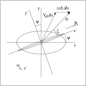
Figure 1: The eccentric ellipse along the $x^{\prime}$ axis corresponds to the diffraction pattern associated with a thin layer of material with a single magnetic field vector whose projection in the plane of the sky, $B_{\perp}$, is along $x^{\prime}$. The projection of the density structures would also appear as eccentric ellipses elongated along $x^{\prime}$. The less eccentric ellipse corresponds to the diffraction pattern resulting from scattering along the entire line of sight. The $y$ axis is defined to be along the short axis of the less eccentric ellipse, which is the long dimension of the corresponding broadened image.

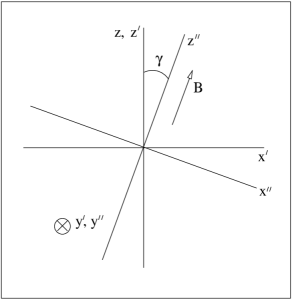
Figure 2: The magnetic field is along $z^{\prime\prime}$, which makes an angle $\gamma$ with the $z$ and $z^{\prime}$ axes.

We assume a GS spectrum for $P_{n_{\rm e}}(\vec{q},z)$ with a sharp cutoff at scales larger than an outer scale $l$ and at scales smaller than an inner scale $d$, i.e., if $l^{-1}<q_{\perp}<d^{-1}$ then

$$P_{n_{\rm e}}(\vec{q},z)=(1/6\pi)\langle\delta n_{\rm e}^{2}\rangle l^{-1/3}q_{\perp}^{-10/3}f\left(\frac{\displaystyle q_{z^{\prime\prime}}}{\displaystyle q_{\perp}^{2/3}l^{-1/3}}\right),$$ (13)

and if $q_{\perp}<l^{-1}$ or $q_{\perp}>d^{-1}$ then $P_{n_{\rm e}}(\vec{q},z)=0$, where

$$f(x)\equiv\left\{\begin{array}[]{ll}1&\mbox{ if $|x|<1$}\\ 0&\mbox{ if $|x|>1$}\end{array}\right.,$$ (14)

and where $q_{\perp}=(q_{x^{\prime\prime}}^{2}+q_{y^{\prime\prime}}^{2})^{1/2}$. The normalization in equation (13) has been chosen so that the mean square density fluctuation is given by $\langle\delta n_{\rm e}^{2}\rangle$.

Noting that

$$q_{x^{\prime\prime}} = q_{x^{\prime}}\cos\gamma-q_{z^{\prime}}\sin\gamma,$$ (15)

$$q_{y^{\prime\prime}} = q_{y^{\prime}},\mbox{ \hskip 8.5359pt and}$$ (16)

$$q_{z^{\prime\prime}} = q_{x^{\prime}}\sin\gamma+q_{z^{\prime}}\cos\gamma,$$ (17)

we find from equations (13) and (14) that $P_{n_{\rm e}}(q_{x^{\prime}},q_{y^{\prime}},q_{z^{\prime}}=0,z)$ is nonzero only when

$$|q_{x^{\prime}}l\sin\gamma|^{3}<q_{x^{\prime}}^{2}l^{2}\cos^{2}\gamma+q_{y^{\prime}}^{2}l^{2}.$$ (19)

The fluctuations that dominate radio-wave scattering typically satisfy $q_{y^{\prime}}l\gg 1$. When $q_{y^{\prime}}l\gg 1$ and $\gamma\gg(q_{y^{\prime}}l)^{-1/3}$ (i.e., the magnetic field is not too closely aligned with the line of sight), the first term on the right-hand side of equation (19) is negligible compared to the second for all allowable values of $q_{x^{\prime}}$, and the upper limit on $q_{x^{\prime}}$ becomes

$$|q_{x^{\prime}}l\sin\gamma|^{3}\lesssim q_{y^{\prime}}^{2}l^{2}.$$ (20)

Thus, when $q_{y^{\prime}}l\gg 1$ and $\gamma\gg(q_{y^{\prime}}l)^{-1/3}$,

$$P_{n_{\rm e}}(q_{x^{\prime}},q_{y^{\prime}},q_{z^{\prime}}=0,z)\simeq\hskip 113.81102pt$$

$$(1/6\pi)\langle\delta n_{\rm e}^{2}\rangle l^{-1/3}q_{y^{\prime}}^{-10/3}f\left(\frac{q_{x^{\prime}}}{q_{y^{\prime}}^{2/3}l^{-1/3}\csc\gamma}\right).$$ (21)

On the other hand, as $\gamma\rightarrow 0$, $P_{n_{\rm e}}$ becomes isotropic in $q_{x^{\prime}}$ and $q_{y^{\prime}}$.

In order to calculate $D_{\phi}$ for different cases, we will first calculate the value of $g(z,\vec{\sigma})$ for various orientations of the magnetic field direction ${\bf\hat{z}^{\prime\prime}}$ relative to the line of sight and the vector $\vec{\sigma}$ separating the two lines of sight in the turbulent medium.

3.1 Value of $g(z,\vec{\sigma})$ when the magnetic field is along the line of sight

When $\sigma$ is in the inertial range ($d\ll\sigma\ll l$) and $\gamma\ll(\sigma/l)^{1/3}$, the dominant contributions to $g(z,\vec{\sigma})$ comes from values of $q_{x^{\prime}}$ and $q_{y^{\prime}}$ satisfying $q_{x^{\prime}}^{2}+q_{y^{\prime}}^{2}\simeq\sigma^{-2}$, for which the value of $f$ in $P_{n_{\rm e}}(q_{x^{\prime}},q_{y^{\prime}},q_{z^{\prime}}=0,z)$ is equal to 1. Thus, when $\sigma$ is in the inertial range ($d\ll\sigma\ll l$) and $\gamma\ll(\sigma/l)^{1/3}$, one can take

$$P_{n_{\rm e}}(q_{x^{\prime}},q_{y^{\prime}},q_{z^{\prime}}=0,z)\simeq(1/6\pi)\langle\delta n_{\rm e}^{2}\rangle l^{-1/3}(q_{x^{\prime}}^{2}+q_{y^{\prime}}^{2})^{-5/3},$$ (22)

which implies that to lowest order in $(\sigma/l)$

$$g(z,\vec{\sigma})=\frac{\Gamma(1/3)}{2^{10/3}\Gamma(5/3)}\langle\delta n_{\rm e}^{2}\rangle l^{-1/3}\sigma^{4/3}.$$ (23)

When $\sigma$ is in the dissipation range ($\sigma\ll d$) and $\gamma\ll(d/l)^{1/3}$, one finds that to lowest order in $(\sigma/d)$ and $(d/l)$

$$g(z,\vec{\sigma})=(1/8)\langle\delta n_{\rm e}^{2}\rangle l^{-1/3}d^{-2/3}\sigma^{2}.$$ (24)

The values of $g$ in equations (23) and (24) are large compared to those that arise from other orientations of $\vec{B}$ due to the increased coherence length of the elongated density structures along the line of sight.

3.2 Value of $g(z,\vec{\sigma})$ when magnetic field is not along the line of sight and $\vec{\sigma}$ is not along ${\bf\hat{x}^{\prime}}$

Let

$$u\equiv q_{y^{\prime}}l,$$ (25)

$$a\equiv\frac{\sigma\cos\zeta}{l}\ll 1,$$ (26)

$$b\equiv\frac{\sigma\sin\zeta}{l}\ll 1,$$ (27)

and let $u_{\rm min}$ be some value of $u$ satisfying

$$1\ll u_{\rm min}\ll|b|^{-1}.$$ (28)

For $\gamma\gg u_{\rm min}^{-1/3}$ and for $u>u_{\rm min}$, $P_{n_{\rm e}}$ is given by equation (21). Thus, for $\gamma\gg u_{\rm min}^{-1/3}$, the contribution to $g(z,\vec{\sigma})$ from $u>u_{\rm min}$ is

$$g(z,\vec{\sigma})=\frac{2\langle\delta n_{\rm e}^{2}\rangle l}{3\pi}\int_{u_{\rm min}}^{l/d}du\,u^{-10/3}\left[u^{2/3}\csc\gamma-\hskip 85.35826pt\right.$$

$$\left.\hskip 85.35826pt\frac{1}{a}\sin(au^{2/3}\csc\gamma)\cos(bu)\right].$$ (29)

If $d\ll\sigma\sin\zeta\ll l$ and $|a|^{3/2}(\csc\gamma)^{3/2}\ll|b|$, which implies that

$$|\zeta|\gg(\sigma/l)^{1/2}(\csc\gamma)^{3/2},$$ (30)

then there exists a $u_{1}<l/d$ such that $au_{1}^{2/3}\csc\gamma\ll 1$ and $|bu_{1}|\gg 1$. The contribution to $g(z,\vec{\sigma})$ from $q_{y^{\prime}}\gg l^{-1}$ is then dominated by values of $u$ in the interval $(u_{\rm min},u_{1})$, in which the integrand in equation (29) can be expanded:

$$g(z,\vec{\sigma})=\frac{2\langle\delta n_{\rm e}^{2}\rangle l}{3\pi}\int_{u_{\rm min}}^{u_{1}}du\,u^{-8/3}\csc\gamma[1-\cos(bu)].$$ (31)

To lowest order the limits of integration can be changed to $(0,\infty)$, which implies that the contribution to $g(z,\vec{\sigma})$ from values of $q_{y^{\prime}}$ much greater than $l^{-1}$ is

$$g(z,\vec{\sigma})=\left[\frac{2}{5\Gamma(5/3)}\right]\langle\delta n_{\rm e}^{2}\rangle\sigma^{5/3}l^{-2/3}\csc\gamma|\sin\zeta|^{5/3}\hskip 85.35826pt$$

$$\mbox{ \hskip 85.35826pt if $d\ll\sigma\sin\zeta\ll l$}.$$ (32)

Although equation (32) was derived assuming $\gamma\gg u_{\rm min}^{-1/3}$, it is approximately valid under the slightly more general condition $\gamma\gg(\sigma|\sin\zeta|/l)^{1/3}$ since $g(z,\vec{\sigma})$ is dominated by values of $q_{y^{\prime}}$ of order $(\sigma|\sin\zeta|)^{-1}$.

As $\zeta\rightarrow 0$, the contribution to $g(z,\vec{\sigma})$ from large $q_{y^{\prime}}$ vanishes, but the contribution from small $q_{y^{\prime}}$ does not. Anticipating the results of the next subsection, we note that in order for the large-$q_{y^{\prime}}$ contribution to dominate and for equation (32) to be accurate when $\sigma\sin\zeta$ is in the inertial range, $\zeta$ must satisfy the condition

$$|\zeta|\gg(\sigma/l)^{1/5}(\sin\gamma)^{3/5}$$ (33)

as well as equation (30).

When $\sigma\sin\zeta$ is in the dissipation range ($\ll d$) and $\gamma\gg(d/l)^{1/3}$, one finds that the contribution to $g(z,\vec{\sigma})$ from $q_{y^{\prime}}\gg l^{-1}$ is to lowest order

$$g(z,\vec{\sigma})=(1/\pi)\langle\delta n_{\rm e}^{2}\rangle l^{-2/3}d^{-1/3}\sigma^{2}\sin^{2}\zeta\csc\gamma\hskip 28.45274pt$$

$$\mbox{ \hskip 85.35826pt if $\sigma\sin\zeta\ll d$}.$$ (34)

In order for the large-$q_{y^{\prime}}$ contribution to dominate over the small-$q_{y^{\prime}}$ contribution, $\zeta$ must be $\gg(d/l)^{1/6}(\sin\gamma)^{1/2}$.

3.3 Value of $g(z,\vec{\sigma})$ when magnetic field is not along the line of sight but $\vec{\sigma}$ is along $\bf\hat{x}^{\prime}$

When $\sigma\sin\zeta$ is in the inertial range, $\gamma\gg(\sigma\sin\zeta\,/l)^{1/3}$, and $|\zeta|\ll(\sigma/l)^{1/5}(\sin\gamma)^{3/5}$, the dominant contribution to $g(z,\vec{\sigma})$ in the Markov approximation comes from $q_{y^{\prime}}\sim l^{-1}$, giving in order of magnitude

$$g(z,\vec{\sigma})\sim\langle\delta n_{\rm e}^{2}\rangle\sigma^{2}l^{-1}.$$ (35)

Equation (35) also holds in the Markov approximation when $\sigma\sin\zeta$ is in the dissipation range, $\gamma\gg(d/l)^{1/3}$, and $|\zeta|\ll(d/l)^{1/6}(\sin\gamma)^{1/2}$. The Markov approximation, however, is formally invalid for density fluctuations at scales $\sim l$, where $l$ is on the order of 1 to 100 pc for typical interstellar conditions. This is because the Markov approximation assumes that

$$\delta\phi=r_{e}\lambda l_{c}\delta n_{\rm e}\ll 1,$$ (36)

where $\delta\phi$ is the phase increment (relative to propagation through the average medium) induced as the wave propagates through one correlation length $l_{c}$ of the density fluctuation $\delta n_{\rm e}$. For the Goldreich-Sridhar spectrum with fractional density fluctuations of order unity at the outer scale $l$, one has $\delta n_{\rm e}\sim n_{e}(l_{c}/l)^{1/3}$. Thus, the Markov approximation is valid only for those density fluctuations with correlation lengths satisfying

$$l_{c}\ll l^{1/4}\lambda^{-3/4}r_{e}^{-3/4}n_{e}^{-3/4}.$$ (37)

For $l=10^{20}$ cm, $\lambda=30$ cm, and $n_{e}=0.1\mbox{ cm}^{-3}$, the Markov approximation is only valid for $l_{c}\ll 10^{14}$ cm. Although the Markov approximation breaks down for the fluctuations at scales larger than $\sim 10^{14}$ cm, we will for simplicity assume that the Markov-approximation results are accurate for the large-scale fluctuations in order of magnitude. In almost all cases, this assumption leads to the conclusion that the large-scale density fluctuations are unimportant for scintillation and angular broadening. The only exception is when all of the density fluctuations are aligned in approximately the same direction, as in section 3.6. In that case, the large-scale fluctuations dominate the angular broadening in the direction parallel to the elongated density structures.

Having determined the values of $g(z,\vec{\sigma})$ for different orientations of the magnetic field relative to $\bf\hat{z}$ and $\vec{\sigma}$, we now turn to calculations of $D_{\phi}$.

3.4 Value of $D_{\phi}$ when there is either significant variation in the magnetic-field direction $\bf\hat{z}^{\prime\prime}$ along the line of sight, or when $\bf\hat{z}^{\prime\prime}$ is not along the line-of-sight and $\bf\hat{x}^{\prime}$ is not along $\vec{\sigma}$

The $z$ integral appearing in equation (3) can be divided into intervals in which (a) the magnetic field $\vec{B}$ is along the line of sight, (b) $\vec{B}$ is not along the line of sight and $\bf\hat{x}^{\prime}$ is not along $\vec{\sigma}$, and (c) $\vec{B}$ is not along the line of sight but $\bf\hat{x}^{\prime}$ is along $\vec{\sigma}$. In intervals of type (a), when $\sigma$ is in the inertial range, the value of the integrand in equation (3) is $\sim(l/\sigma)^{1/3}$ times larger than in intervals of type (b). However, intervals of type (a) [for which $\gamma<(\sigma/l)^{1/3}$] are about a factor of $(\sigma/l)^{2/3}$ less common than intervals of type (b) when the field direction varies significantly along the line of sight in a random manner, and thus intervals of type (a) do not contribute significantly to $D_{\phi}$. Intervals of type (c) are much less common than intervals of type (b), and in addition the integrand in equation (3) is smaller in intervals of type (c) than in intervals of type (b). Thus, $D_{\phi}$ is dominated by intervals of type (b), both when there is significant random variation in the field direction along the line of sight and when the field direction is fixed in a single direction of type (b).

When $d\ll\sigma\ll l$, for most values of $\zeta$ one also has $d\ll\sigma\sin\zeta\ll l$, the condition under which $g(z,\vec{\sigma})$ is given by equation (32). Thus, when $\sigma$ is in the inertial range,

$$D_{\phi}=\frac{8\pi}{5\Gamma(5/3)}r_{e}^{2}\lambda^{2}\int_{0}^{L}dz(\langle\delta n_{\rm e}^{2}\rangle l^{-2/3}\csc\gamma|\sin\zeta|^{5/3}\sigma^{5/3})$$

$$\mbox{ \hskip 85.35826pt if $d\ll\sigma\ll l$},$$ (38)

where the integration excludes segments of the line of sight for which $\gamma\lesssim(\sigma/l)^{1/3}$. Similar arguments show that when $\sigma$ is in the dissipation range, the $z$ integral in equation (3) is dominated by intervals in which $g(z,\vec{\sigma})$ is given by equation (34), giving

$$D_{\phi}=4r_{e}^{2}\lambda^{2}\int_{0}^{L}dz\,(\langle\delta n_{\rm e}^{2}\rangle l^{-2/3}d^{-1/3}\sigma^{2}\sin^{2}\zeta\csc\gamma)$$

                           if $$\sigma\ll d$$, (39)

where the integration excludes segments of the line of sight for which $\gamma\lesssim(d/l)^{1/3}$.

A subtlety not addressed in this paper is that $\sigma$ can be within the inertial range of the turbulence over part of the line of sight and within the dissipation range over the remainder of the line of sight. For simplicity it will be assumed that if $\sigma$ is in the inertial range at either the source or at the observer, then the inertial-range formulas can be used for the entire line of sight. For example, if $\delta r$ is in the inertial range and $\delta t=0$, then $\sigma$ is taken to be in the inertial range along the entire line of sight, although in fact it is in the dissipation range sufficiently close to the source.

From equations (8), (9), (10) and (38), one finds that for $d\ll\sigma\ll l$,

$$l_{{\rm d},x}=\left(\int_{0}^{1}d\xi L\eta_{\rm gs}\csc\gamma|\sin\psi|^{5/3}\xi^{5/3}\right)^{-3/5},$$ (40)

$$l_{{\rm d},y}=\left(\int_{0}^{1}d\xi L\eta_{\rm gs}\csc\gamma|\cos\psi|^{5/3}\xi^{5/3}\right)^{-3/5},\mbox{ \hskip 8.5359pt and}$$ (41)

$$t_{d}=\left[\int_{0}^{1}d\xi L\eta_{\rm gs}\csc\gamma|\sin\zeta|^{5/3}|(1-\xi)\vec{V}_{\rm p}+\xi\vec{V}_{\rm obs}|^{5/3}|\right]^{-3/5},$$ (42)

where $\eta_{\rm gs}=[8\pi/5\Gamma(5/3)]r_{e}^{2}\lambda^{2}\langle\delta n_{\rm e}^{2}\rangle l^{-2/3}$, $\xi=z/L$, and the integration excludes segments of the line of sight in which $\gamma\lesssim(\sigma/l)^{1/3}$. Equations (40) and (41) show that the length scale of the diffraction pattern tends to be dominated by fluctuations near the observer. If $V_{\rm p}\gg V_{\rm obs}$, then equation (42) shows that the time scale of the diffraction pattern tends to be dominated by fluctuations near the source.

3.5 Special case: homogeneous extended medium with a statistically isotropic random magnetic field direction

Let us suppose that the magnetic-field direction varies randomly in an isotropic manner along the line of sight, and that $\langle\delta n_{\rm e}^{2}\rangle$, $l$, and $d$ are constant along the line of sight. We have already assumed that $l\ll L$, which implies that in the $z$ integral in equation (38) we can average over the direction of $\vec{B}$ while holding $z$ constant to a good approximation. With

$$\alpha \equiv \frac{32\pi^{2}}{5\Gamma(5/3)}\int_{0}^{\pi/2}d\zeta(\sin\zeta)^{5/3},$$ (43)

$$\xi \equiv \frac{z}{L},\mbox{ \hskip 8.5359pt and}$$ (44)

$$H \equiv (r_{e}^{2}\lambda^{2}\langle\delta n_{\rm e}^{2}\rangle L)^{-1},$$ (45)

one finds that

$$D_{\phi}=\alpha H^{-1}l^{-2/3}\int_{0}^{1}d\xi\,|(\vec{\delta r}-\vec{V}_{\rm p}\delta t+\vec{V}_{\rm obs}\delta t)\xi+\vec{V}_{\rm p}\delta t|^{5/3}$$

                           if $$d\ll\sigma\ll l$$. (46)

When $\delta t=0$, or $V_{\rm p}=V_{\rm obs}=0$,

$$D_{\phi}=(3/8)\alpha H^{-1}l^{-2/3}\delta r^{5/3}.\mbox{ \hskip 8.5359pt if $d\ll\delta r\ll l$.}$$ (47)

The diffraction pattern in this case is isotropic, with

$$l_{{\rm d},x}=l_{{\rm d},y}=\left(\frac{8}{3\alpha}\right)^{3/5}H^{3/5}l^{2/5}\mbox{ if $d\ll l_{{\rm d},x}=l_{{\rm d},y}\ll l$.}$$ (48)

When $\sigma$ is in the dissipation range, one finds that

$$D_{\phi}=4\pi^{2}H^{-1}l^{-2/3}d^{-1/3}\hskip 8.5359pt\times$$

$$[(1/3)|\vec{\delta r}+\vec{V}_{\rm obs}\delta t-\vec{V}_{\rm p}\delta t|^{2}+\vec{\delta r}\cdot\vec{V}_{\rm p}\delta t+\vec{V}_{\rm p}\cdot\vec{V}_{\rm obs}\delta t^{2}]\mbox{ \hskip 8.5359pt if $\sigma\ll d$},$$ (49)

$$l_{{\rm d},x}=l_{{\rm d},y}=\left(\frac{3}{4\pi^{2}}\right)^{1/2}H^{1/2}l^{1/3}d^{1/6}\mbox{ \hskip 8.5359pt if $l_{{\rm d},x}=l_{{\rm d},y}\ll d$},$$ (50)

and

$$t_{d}=\left(\frac{3}{4\pi^{2}}\right)^{1/2}\frac{H^{1/2}l^{1/3}d^{1/6}}{(V_{\rm obs}^{2}+\vec{V}_{\rm obs}\cdot\vec{V}_{\rm p}+V_{\rm p}^{2})^{1/2}}$$

$$\mbox{ \hskip 85.35826pt if $l_{{\rm d},x}=l_{{\rm d},y}\ll d$}.$$ (51)

3.6 Special case: one thin scattering screen with a single direction of $\vec{B}$

In this section, it is assumed that all of the electron density fluctuations lie within a screen of thickness $\Delta z\ll l\ll L$. The magnetic field direction thus does not rotate very much within the screen, and the density fluctuations are aligned in the same direction. The screen is taken to be a distance $z$ from the source. Upon defining

$$h\equiv(r_{e}^{2}\lambda^{2}\Delta z\langle\delta n_{\rm e}^{2}\rangle)^{-1}$$ (52)

(for $\lambda=10$ cm, $\Delta z=10^{18}$ cm, and $\langle\delta n_{\rm e}^{2}\rangle=1\mbox{ cm}^{-6}$, $h=1.3\times 10^{5}$ cm), one finds that

$$l_{{\rm d},y}=\left(\frac{5\Gamma(5/3)}{8\pi}\right)^{3/5}h^{3/5}l^{2/5}(\sin\gamma)^{3/5}\frac{L}{z}\mbox{ \hskip 8.5359pt if $d\ll zl_{{\rm d},y}/L\ll l$}.$$ (53)

To obtain an approximate value for $l_{{\rm d},x}$, one must use equation (35) to obtain

$$l_{{\rm d},x}\sim h^{1/2}l^{1/2}\frac{L}{z}.$$ (54)

Equation (54) holds whether $zl_{{\rm d},x}/L$ is in the dissipation range or the inertial range. As discussed in section 3.3, we are unable to determine how $l_{{\rm d},x}$ changes with $\gamma$ as $\csc\gamma$ becomes large. When $\csc\gamma$ is of order unity (e.g., $\lesssim 4$) the axial ratio of the anisotropic diffraction pattern and broadened image is given by

$$\frac{\theta_{s,y}}{\theta_{s,x}}=\frac{l_{{\rm d},x}}{l_{{\rm d},y}}\sim\left(\frac{l}{h}\right)^{1/10}\mbox{ \hskip 8.5359pt if $d\ll zl_{{\rm d},y}/L\ll l$},$$ (55)

ignoring factors of order unity. The axial ratio of the density structures in the Goldreich-Sridhar spectrum that dominate the diffraction pattern is

$$[l/(zl_{{\rm d},y}/L)]^{1/3}\sim\left(\frac{l}{h}\right)^{1/5}\mbox{ \hskip 8.5359pt if $d\ll zl_{{\rm d},y}/L\ll l$}.$$ (56)

Thus, for $\csc\gamma$ of order unity, the axial ratio of the diffraction pattern is roughly the square root of the axial ratio of the turbulent structures that dominate the scattering at the scale of the diffraction pattern (i.e. turbulent structures with $q_{y^{\prime}}^{-1}\sim zl_{{\rm d},y}/L$). It should be noted, however, that this result follows from applying the Markov approximation to the outer-scale density fluctuations, for which the approximation is formally invalid. There exist other anisotropic power spectra for which the axial ratio of the diffraction pattern arising from a thin screen equals the axial ratio of the density structures. For example, if $P_{n_{\rm e}}(q_{x^{\prime\prime}},q_{y^{\prime\prime}},q_{z^{\prime\prime}})\propto[q_{x^{\prime\prime}}^{2}+q_{y^{\prime\prime}}^{2}+(R^{\prime\prime})^{2}q_{z^{\prime\prime}}^{2}]^{-\beta/2}$ where $R^{\prime\prime}$ and $\beta$ are constants, $R^{\prime\prime}\gg 1$, and $\beta<4$, and if $\csc\gamma$ is of order 1, then the axial ratio of the diffraction pattern is $\sim R^{\prime\prime}$ (Backer & Chandran 2000). Similarly, Narayan & Hubbard (1988) showed that if the two-dimensional power spectrum of the phase fluctuations in a thin scattering screen is $\propto[(R^{\prime\prime})^{2}q_{x}^{2}+q_{y}^{2}]^{-\beta/2}$ with $\beta<4$, then the axial ratio of the associated diffraction pattern is $R^{\prime\prime}$. The key difference between these axial ratios and the axial ratios for a GS spectrum is the following: although the image broadening along the $y$ direction for a GS spectrum is dominated by highly anisotropic small-scale fluctuations, the image broadening along the $x$ direction for a GS spectrum is dominated by the large-scale fluctuations. Since the image broadening along $x$ is enhanced relative to the amount of image broadening arising solely from the small-scale density structures, the image is less anisotropic than the density structures.

The scintillation time scale $t_{d}$ is given by

$$t_{d}=\left[\frac{5\Gamma(5/3)}{8\pi}\right]^{3/5}\frac{h^{3/5}l^{2/5}|\csc\zeta|(\sin\gamma)^{3/5}}{V_{\rm eff}}$$

$$\mbox{ \hskip 85.35826pt if $d\ll zV_{\rm eff}t_{d}/L\ll l$}.$$ (57)

However, as $\zeta\rightarrow 0$, $t_{d}$ does not approach $\infty$ but instead reaches a maximum value when $D_{\phi}$ is determined using equation (35):

$$t_{d,\rm max}\sim\frac{h^{1/2}l^{1/2}}{V_{\rm eff}}.$$ (58)

If $|\vec{V}_{\rm eff}$ is constant but $\zeta$ varies continuously through a $360^{\circ}$ interval during the course of either the earth’s orbit around the sun or the orbit of a binary pulsar, then the ratio of the maximum to minimum scintillation times when $\csc\gamma$ is of order unity is given by

$$\frac{t_{d,\rm max}}{t_{d,\rm min}}\simeq\left(\frac{l}{h}\right)^{1/10}.$$ (59)

For $zl_{{\rm d},y}/L$ in the dissipation range, one finds that

$$l_{{\rm d},y}=(1/2)h^{1/2}l^{1/3}d^{1/6}(\sin\gamma)^{1/2}\frac{L}{z}\mbox{ \hskip 8.5359pt if $zl_{{\rm d},y}/L\ll d$}.$$ (60)

Since equation (54) applies in the dissipation range, the axial ratio of the diffraction pattern and broadened image for $\csc\gamma$ of order unity is given by

$$\frac{\theta_{s,y}}{\theta_{s,x}}=\frac{l_{{\rm d},x}}{l_{{\rm d},y}}\sim\left(\frac{l}{d}\right)^{1/6}\mbox{ if $zl_{{\rm d},y}/L\ll d$},$$ (61)

which again, is approximately the square root of the axial ratio of the turbulent structures at scale $d$ that dominate the scattering for $zl_{{\rm d},y}/L\ll d$. The scintillation time scale is

$$t_{d}=\frac{h^{1/2}l^{1/3}d^{1/6}(\sin\gamma)^{1/2}\csc\zeta}{2V_{\rm eff}}\mbox{ \hskip 8.5359pt if $zl_{{\rm d},y}/L\ll d$.}$$ (62)

As $\zeta\rightarrow 0$, $t_{d}$ stops increasing after reaching the value given in equation (58). Again, if $V_{\rm eff}$ is constant but $\zeta$ varies continuously through a $360^{\circ}$ interval during the course of either the earth’s orbit around the sun or the orbit of a binary pulsar, then the ratio between the maximum and minimum scintillation times when $\csc\gamma$ is of order unity is given by

$$\frac{t_{d,\rm max}}{t_{d,\rm min}}\simeq\left(\frac{l}{d}\right)^{1/6}.$$ (63)

3.7 Special case: thin scattering screen in which the direction of magnetic field in plane of sky rotates through an angle $\Delta\psi$

In this section, it is assumed that the scattering medium extends from $z=z_{1}$ to $z=z_{1}+\Delta z$, with $\Delta z\ll L$. It is assumed that $\langle\delta n_{\rm e}^{2}\rangle$, $l$, and $\gamma$ are constant within the screen, that $\sigma$ is in the inertial range of the density fluctuations, and that $\gamma\gg(\sigma\sin\zeta/l)^{1/3}$. The angle $\psi$ between the projection of the magnetic field in the plane of the sky and the $x$ axis is given by

$$\psi=-\frac{\Delta\psi}{2}+\frac{(z-z_{1})\Delta\psi}{\Delta z}.$$ (64)

The value of $\Delta\psi$ is conceptually equivalent to $\Delta z/l$. It is assumed that

$$\Delta\psi\gg R^{-1/2},$$ (65)

where $R$ is the axial ratio of the small-scale density structures that dominate the scattering. This means that for any direction of $\vec{\sigma}$, portions of the line of sight of type (c) in section 3.4 (for which $\vec{\sigma}$ is nearly along the direction of ${\bf B}$ in the plane of the sky) contribute a negligible amount to $D_{\phi}$, and $D_{\phi}$ is given by equation (38). From this it follows that

$$\frac{l_{{\rm d},x}}{l_{{\rm d},y}}=\left[\frac{\displaystyle\int_{0}^{\Delta\psi/2}d\psi\,|\cos\psi|^{5/3}}{\displaystyle\int_{0}^{\Delta\psi/2}d\psi\,|\sin\psi|^{5/3}}\right]^{3/5}.$$ (66)

When $|\Delta\psi|\ll 1$, equation (66) reduces to

$$\frac{l_{{\rm d},x}}{l_{{\rm d},y}}\simeq\frac{2(8/3)^{3/5}}{\Delta\psi}\simeq\frac{3.6}{\Delta\psi}.$$ (67)

Equations (66) and (67) are plotted in figure 3. If $|\vec{V}_{\rm eff}|$ is constant during one orbit of the earth around the Sun or one orbit of a binary pulsar, then the ratio of the maximum to minimum scintillation times $t_{\rm d,max}/t_{\rm d,min}$ during the course of one orbit is also given by

$$\frac{t_{\rm d,max}}{t_{\rm d,min}}=\left[\frac{\displaystyle\int_{0}^{\Delta\psi/2}d\psi\,|\cos\psi|^{5/3}}{\displaystyle\int_{0}^{\Delta\psi/2}d\psi\,|\sin\psi|^{5/3}}\right]^{3/5},$$ (68)

and when $|\Delta\psi|\ll 1$,

$$\frac{t_{\rm d,max}}{t_{\rm d,min}}\simeq\frac{2(8/3)^{3/5}}{\Delta\psi}\simeq\frac{3.6}{\Delta\psi}.$$ (69)

The scintillation time reaches its maximum value when the sight line moves parallel to $\hat{x}$, the direction in which the density fluctuations are most elongated, and reaches its minimum when the sight line moves along $\hat{y}$.

Figure 3: Axial ratio of the diffraction pattern and broadened image of a point source when the magnetic field direction in the plane of the sky rotates through an angle $\Delta\psi$ within the scattering screen. The solid line represents equation (66), and the dashed line represents equation (67), which is derived assuming $|\Delta\psi|\ll 1$.

4 Summary of results

In this paper, we assume a GS spectrum (Goldreich & Sridhar 1995) of electron density fluctuations in the ISM. We then calculate general formulas for the wave phase structure function, visibility, angular broadening, diffraction-pattern length scales, and scintillation time scale for arbitrary distributions of turbulence along the line of sight, and specialize these formulas to idealized cases. Our main results are as follows:

(1) Unless the magnetic field is closely aligned with the line of sight over a much greater fraction of the line of sight than is expected for random magnetic fields, the scaling of the wave phase structure function $D_{\phi}$ with baseline $\delta r$ is $D_{\phi}\propto(\delta r)^{5/3}$ for $\delta r$ in the inertial range of the turbulence, and $D_{\phi}\propto(\delta r)^{2}$ for $\delta r$ smaller than the dissipation scale or inner scale of the turbulence, just as for an isotropic Kolmogorov spectrum of density fluctuations.

(2) If the magnetic field were closely aligned with the line of sight [within an angle $\sim(\delta r/l)^{1/3}$ if $\delta r$ is in the inertial range, and $\sim(d/l)^{1/3}$ if $\delta r$ is in the dissipation range] over more than a minimum-threshold fraction of the line of sight, scattering would be dominated by that fraction of the line of sight and $D_{\phi}$ would be proportional to $(\delta r)^{4/3}$ if $\delta r$ were in the inertial range, and to $(\delta r)^{2}$ if $\delta r$ were smaller than the dissipation scale. The minimum-threshold fraction is small [$\sim(\delta r/l)^{1/3}$ if $\delta r$ is in the inertial range, or $\sim(d/l)^{1/3}$ if $\delta r$ is in the dissipation range], but much larger than expected for randomly varying magnetic fields. The increase in scattering when $\vec{B}$ becomes aligned along the line of sight is due to the increased coherence length of the elongated density structures along the line of sight.

(3) Angular broadening is most anisotropic when scattering occurs within a thin screen in which the magnetic field has a single direction. In this case, the axial ratio of the broadened image of a point source in the Markov approximation is approximately the square root of the axial ratio of the density fluctuations that dominate the scattering, provided that $\csc\gamma$ is of order unity (e.g. $\lesssim 4$), where $\gamma$ is the angle between the magnetic field and the line of sight. We have not found the dependence of the axial ratio on $\gamma$ when $\csc\gamma$ is large, although we do show that if $\gamma=0$ the broadened image is isotropic.

(4) If the scattering medium is confined to a homogeneous thin screen of thickness $\Delta z\ll L$, and if the direction of the magnetic field in the plane of the sky rotates through an angle $\Delta\psi\gg R^{-1/2}$ along the line of sight from one side of the screen to the other, where $R$ is the axial ratio of the density fluctuations that dominate the scattering, then the axial ratio of the observed image of a point source is $\simeq 3.6/\Delta\psi$. [This formula is derived assuming $\Delta\psi\ll 1$, but closely approximates (to within 15%) the more general formula, equation (66), for $\Delta\psi$ as large as $\pi$.] This indicates that even a moderate variation in the field direction within the scattering medium can dramatically reduce the axial ratio of an angularly broadened imaged. If the field direction along the line of sight to a source varies significantly, the resulting angular-broadening anisotropy is determined by the amount of variation in the field direction rather than by the degree of anisotropy of the density fluctuations.

(5) When the magnetic field in the scattering medium has a single direction or rotates through a relatively small angle $\Delta\psi$, the scintillation time is longest when the sight line moves along the direction of greatest elongation of the electron density fluctuations in the scattering medium, and shortest when the sight line moves orthogonal to the direction of greatest elongation of the density structures. This gives rise to an observable modulation of the scintillation time during the course of either the Earth’s orbit around the Sun, or of a binary pulsar’s orbit. When the speed of the sight line in the plane of the sky $V_{\rm eff}$ in the scattering medium (assumed to be a thin screen) is constant during the orbit, the ratio of the maximum to minimum scintillation times $t_{\rm d,max}/t_{\rm d,min}$ is the same as the axial ratio of the broadened image of a point source, when the magnetic field has a single direction in the thin screen as well as when the magnetic field rotates through an angle $\Delta\psi$. If the field direction along the line of sight to a source varies significantly, the degree of variation in the scintillation time is determined by the amount of variation in the field direction rather than by the degree of anisotropy of the density fluctuations.

(6) The diffraction-pattern length scales and angular broadening are more sensitive to fluctuations near the earth than to fluctuations near the pulsar. The time scale for diffractive scintillations is more sensitive to fluctuations near the pulsar if the pulsar speed significantly exceeds the speed of the observer with respect to the interstellar turbulence.

Appendix A Derivation of equations for visibility and intensity correlation function for a moving observer and moving point source

In this appendix we derive equations (2) through (7) for the visibility and intensity correlation function for a moving point source and moving observer. In several places, the derivation is identical to the corresponding calculation for plane waves incident upon a turbulent medium and observer that are at rest, and the reader will be referred to Lee & Jokipii (1975a,b) for the details.

We work in the rest frame of the source, and start with the scalar wave equation for electromagnetic waves propagating in a cold non-magnetized plasma (Faraday rotation is ignored),

$$\nabla^{2}E-\frac{1}{c^{2}}\frac{\partial^{2}E}{\partial t^{2}}-\frac{\omega_{p}^{2}}{c^{2}}E=0,$$ (A1)

where

$$\omega_{p}^{2}=\frac{4\pi n_{e}e^{2}}{m_{e}}.$$ (A2)

We look for solutions that are approximately spherical waves,

$$E=ue^{i(kr-\omega t)},$$ (A3)

with

$$u\rightarrow 1\mbox{ \hskip 8.5359pt as \hskip 8.5359pt }r\rightarrow 0,$$ (A4)

where $(r,\theta,\phi)$ are spherical coordinates centered on the source, and, in the notation of Lee & Jokipii (1975a),

$$k^{2}=\frac{\omega^{2}\epsilon_{0}}{c^{2}},\hskip 14.22636pt\epsilon_{0}=\langle\epsilon_{\ast}\rangle,\mbox{ \hskip 8.5359pt and \hskip 8.5359pt }\epsilon_{\ast}=1-\frac{\omega_{p}^{2}}{\omega^{2}}.$$ (A5)

The angled brackets denote an ensemble average over the turbulent density fluctuations. We also define

$$\epsilon=-\frac{4\pi\delta n_{\rm e}r_{e}}{k^{2}}$$ (A6)

to be the fractional fluctuations in the dielectric constant $\epsilon_{\ast}$, where $r_{e}$ is the classical electron radius $e^{2}/(m_{e}c^{2})$, so that

$$\epsilon_{\ast}=\epsilon_{0}(1+\epsilon).$$ (A7)

We make the “parabolic approximations,”

$$k\frac{\partial u}{\partial r}\gg\frac{\partial^{2}u}{\partial r^{2}}\hskip 14.22636pt\mbox{ and}\hskip 14.22636pt\omega\frac{\partial u}{\partial t}\gg\frac{\partial^{2}u}{\partial t^{2}},$$ (A8)

and using equations (A1) through (A8) find that

$$2ik\left(\frac{\partial u}{\partial r}+\frac{1}{v_{g}}\frac{\partial u}{\partial t}\right)+\nabla_{\perp}^{2}u+\epsilon k^{2}u=0,$$ (A9)

where

$$v_{g}=c\sqrt{\epsilon_{0}},$$ (A10)

and

$$\nabla_{\perp}^{2}=\frac{1}{r^{2}}\left[\frac{1}{\sin\theta}\frac{\partial}{\partial\theta}\left(\sin\theta\frac{\partial}{\partial\theta}\right)+\frac{1}{\sin^{2}\theta}\frac{\partial^{2}}{\partial\phi^{2}}\right].$$ (A11)

We then transform coordinates from $(r,\theta,\phi,t)$ to $(z,\theta,\phi,s)$, where

$$z=r\hskip 8.5359pt\mbox{ and}\hskip 8.5359pts=r-v_{g}t.$$ (A12)

Points with a constant $s$ are all those values of $r$ and $t$ associated with the wavefront that arrives at the observer at the time $t=(L-s)/v_{g}$, where $L$ is the distance from source to observer. In terms of $z$ and $s$ and the shorthand notation defined in table 1, equation (A9) can be written

$$2ik\frac{\partial u_{1}}{\partial z}+\nabla_{\perp,1}^{2}u_{1}+\epsilon_{1}k^{2}u_{1}=0.$$ (A13)

Equation (A13) is of the same form as equation (7) of Lee & Jokipii (1975a).

Abbreviation	Meaning
$u_{i}$	$u(z,\theta_{i},\phi_{i},s_{i})$
$u_{i}^{\prime}$	$u(z^{\prime},\theta_{i},\phi_{i},s_{i})$
$\epsilon_{i}$	$\epsilon(z,\theta_{i},\phi_{i},s_{i})$
$\epsilon_{i}^{\prime}$	$\epsilon(z^{\prime},\theta_{i},\phi_{i},s_{i})$
$\nabla_{\perp,i}^{2}$	$\displaystyle\frac{1}{z^{2}}\left[\frac{1}{\sin\theta_{i}}\frac{\partial}{\partial\theta_{i}}\left(\sin\theta_{i}\frac{\partial}{\partial\theta_{i}}\right)+\frac{1}{\sin^{2}\theta_{i}}\frac{\partial^{2}}{\partial\phi_{i}^{2}}\right]$

Table 1: Shorthand notation, where $i=1,2,3,$ or 4.

Taking the complex conjugate of equation (A13), and evaluating the terms at $\theta_{2}$, $\phi_{2}$, and $s_{2}$, one can write

$$2ik\frac{\partial u_{2}^{\ast}}{\partial z}-\nabla_{\perp,\,2}^{2}u_{2}^{\ast}-\epsilon_{2}k^{2}u_{2}^{\ast}=0.$$ (A14)

Multiplying equation (A13) by $u_{2}^{\ast}$ and equation (A14) by $u_{1}$ and adding, taking the ensemble average, and noting that for statistically homogeneous density fluctuations $\nabla_{\perp,1}^{2}\langle u_{1}u_{2}^{\ast}\rangle=\nabla_{\perp,2}^{2}\langle u_{1}u_{2}^{\ast}\rangle$, we find that

$$2ik\frac{\partial}{\partial z}\langle u_{1}u_{2}^{\ast}\rangle+k^{2}\langle(\epsilon_{1}-\epsilon_{2})u_{1}u_{2}^{\ast}\rangle=0.$$ (A15)

We now make the Markov approximation, in which we assume that the correlation length of the density fluctuations $l_{\epsilon}$ is much smaller than the length $l_{u}$ along the line of sight over which $u$ changes significantly. We then follow a procedure analogous to the one described in appendix A of Lee & Jokipii (1975a) to show that

$$\langle(\epsilon_{1}-\epsilon_{2})u_{1}u_{2}^{\ast}\rangle=\frac{ik\langle u_{1}u_{2}^{\ast}\rangle}{2}\int_{-\infty}^{z}dz_{1}(\langle\epsilon_{1}\epsilon_{1}^{\prime}\rangle+\langle\epsilon_{2}\epsilon_{2}^{\prime}\rangle-\langle\epsilon_{1}\epsilon_{2}^{\prime}\rangle-\langle\epsilon_{2}\epsilon_{1}^{\prime}\rangle).$$ (A16)

To evaluate the right-hand side of equation (A16), we first define $\alpha$ according to the equation

$$\theta=\frac{\pi}{2}+\alpha.$$ (A17)

We restrict our attention to values of $\alpha$ and $\phi$ satisfying

$$|\alpha|\ll 1\mbox{ \hskip 8.5359pt and \hskip 8.5359pt }|\phi|\ll 1.$$ (A18)

We then introduce Cartesian coordinates $(x,y)$ in the plane perpendicular to the line of sight, with

$$x=z\alpha\mbox{ \hskip 8.5359pt and \hskip 8.5359pt}y=z\phi.$$ (A19)

(Note: the $xyz$ coordinates used here are not related to $\theta$ and $\phi$ in the conventional way. For example, the $z$ axis corresponds not to $\theta=0$, but instead to $\theta=\pi/2$ and $\phi=0$.) We also make a two scale approximation along the line of sight, dividing the dependence of the variables on the radial coordinate into two parts: a dependence on $Z$ reflecting variations over scales $\sim l_{\epsilon}$, and a dependence on $z$ reflecting variations over scales $\gg l_{\epsilon}$. The integral in equation (A16) effectively extends over a distance $\sim l_{\epsilon}\ll z$, and so in calculating $x$ and $y$ for $\epsilon_{1}^{\prime}$ and $\epsilon_{2}^{\prime}$ we can use $z$ in place of $z^{\prime}$ in equation (A19) with only small error. Defining $\vec{x}\equiv x\hat{x}+y\hat{y}+Z\hat{z}$, and assuming statistical homogeneity and stationarity, we can write

$$\langle\delta n_{\rm e}(\vec{x}_{1},t_{1};z)\delta n_{\rm e}(\vec{x}_{2},t_{2};z)\rangle\equiv Q(\vec{x}_{1}-\vec{x}_{2},t_{1}-t_{2};z).$$ (A20)

We assume that the density fluctuations are static in the rest frame of the turbulent medium, which is reasonable since the Lagrangian correlation time of the density fluctuations that dominate scintillation is small in the GS theory compared to the time for the line of sight to sweep across such a fluctuation. This gives

$$Q(\vec{x},t;z)=G(\vec{x}-\vec{U}_{m}t;z),$$ (A21)

where $\vec{U}_{m}$ is the uniform velocity of the turbulent medium with respect to the source, and $G(\vec{x};z)$ is the spatial correlation function of the density structures in the rest frame of the turbulent medium, which is the inverse Fourier transform of the density power spectrum $P_{n_{\rm e}}$:

$$G(\vec{x};z)=\int d^{3}q\,e^{i\vec{q}\cdot\vec{x}}P_{n_{\rm e}}(\vec{q};z).$$ (A22)

Defining

$$H_{ij}\equiv\int_{-\infty}^{z}dz^{\prime}\langle\epsilon_{i}\epsilon_{j}^{\prime}+\epsilon_{j}\epsilon_{i}^{\prime}\rangle,$$ (A23)

we find that

$$H_{ij}=\frac{32\pi^{3}r_{e}^{2}}{k^{4}}\int d^{3}q\,P_{n_{\rm e}}(\vec{q};z)e^{i\vec{q}\cdot\vec{p}_{ij}}\delta\left(\vec{q}\cdot\left[\hat{z}-\frac{\vec{U}_{m}}{v_{g}}\right]\right),$$ (A24)

where

$$\vec{p}_{ij}=z(\alpha_{i}-\alpha_{j})\hat{x}+z(\phi_{i}-\phi_{j})\hat{y}+\frac{(s_{i}-s_{j})\vec{U}_{m}}{v_{g}}.$$ (A25)

The presence of the $\vec{U_{m}}/v_{g}$ term in the delta function in equation (A24) is due to aberration—in the frame of reference of the turbulent fluctuations, the wave appears to be moving in a direction slightly offset from the line of sight. Since $U_{m}\ll v_{g}$, this effect is small and can be ignored, and the delta function can be written $\delta(k_{z})$. Equation (A24) thus reduces to

$$H_{ij}=\frac{32\pi^{3}r_{e}^{2}}{k^{4}}\int\int dq_{x}dq_{y}\,P_{n_{\rm e}}(q_{x},q_{y},q_{z}=0;z)e^{i\vec{k}\cdot\vec{\sigma}_{ij}},$$ (A26)

where

$$\vec{\sigma}_{ij}=z(\alpha_{i}-\alpha_{j})\hat{x}+z(\phi_{i}-\phi_{j})\hat{y}+\frac{(s_{i}-s_{j})\vec{U}_{m,\perp}}{v_{g}},$$ (A27)

and where $\vec{U}_{m\,\perp}$ is the component of $\vec{U}_{m}$ perpendicular to the line of sight.

Equations (A15), (A16), (A23), and (A26) imply that

$$\frac{\partial}{\partial z}\langle u_{1}u_{2}^{\ast}\rangle=-2\pi r_{e}^{2}\lambda^{2}g(z,\vec{\sigma}_{12})\langle u_{1}u_{2}^{\ast}\rangle.$$ (A28)

If the correlated observations are taken at locations that are separated in the observer’s rest frame by a displacement $\vec{\delta r}=\delta x\hat{x}+\delta y\hat{y}+\delta z\hat{z}$ and at times that are separated by a time interval $\delta t$, then

$$L(\alpha_{1}-\alpha_{2}) = \delta x+U_{\rm obs,x}\delta t,$$ (A29)

$$L(\phi_{1}-\phi_{2}) = \delta y+U_{\rm obs,y}\delta t,\mbox{ \hskip 8.5359pt and}$$ (A30)

$$s_{1}-s_{2} = -v_{g}(t_{1}-t_{2}).$$ (A31)

Because $u$ changes much more slowly along the line of sight than across the line of sight, $\delta z$ and $U_{\rm obs,z}$ can be neglected. Defining $V_{p}$ and $V_{\rm obs}$ as the velocities of the source and observer perpendicular to the line of sight measured in the rest frame of the turbulent medium, one has

$$\vec{U}_{m,\perp}=-\vec{V}_{p},$$ (A33)

$$\vec{U}_{\rm obs,\perp}=-\vec{V}_{p}+\vec{V}_{\rm obs},$$ (A34)

and

$$\vec{\sigma}_{12}=\frac{z}{L}(\vec{\delta r}+\vec{V}_{\rm obs}\delta t)+\left(1-\frac{z}{L}\right)\vec{V}_{p}\delta t.$$ (A35)

Integrating equation (A28) and using equations (A4) and (A35), one obtains equation (2).

To derive the intensity correlation function, we define

$$\Gamma_{2,2}=\langle u_{1}u_{2}u_{3}^{\ast}u_{4}^{\ast}\rangle.$$ (A36)

Using the same procedure used to derive equation (A15), one obtains

$$2ik\frac{\partial\Gamma_{2,2}}{\partial z}+(\nabla_{\perp,1}^{2}+\nabla_{\perp,2}^{2}-\nabla_{\perp,3}^{2}-\nabla_{\perp,4}^{2})\Gamma_{2,2}+k^{2}\langle(\epsilon_{1}+\epsilon_{2}-\epsilon_{3}-\epsilon_{4})u_{1}u_{2}u_{3}^{\ast}u_{4}^{\ast}\rangle=0.$$ (A37)

Using the Markov approximation, we find that

$$\langle(\epsilon_{1}+\epsilon_{2}-\epsilon_{3}-\epsilon_{4})u_{1}u_{2}u_{3}^{\ast}u_{4}^{\ast}\rangle=\frac{ik\Gamma_{2,2}}{2}(2H_{11}+H_{12}+H_{34}-H_{13}-H_{14}-H_{23}-H_{24}),$$ (A38)

which gives

$$\frac{\partial\Gamma_{2,2}}{\partial z}=\frac{i}{2k}\left(\nabla_{\perp,1}^{2}+\nabla_{\perp,2}^{2}-\nabla_{\perp,3}^{2}-\nabla_{\perp,4}^{2}\right)\Gamma_{2,2}+\frac{k^{2}\Gamma_{2,2}}{4}\left(2H_{11}+H_{12}+H_{34}-H_{13}-H_{14}-H_{23}-H_{24}\right).$$ (A39)

To an excellent approximation,

$$\nabla_{\perp,i}^{2}\simeq\frac{1}{z^{2}}\left(\frac{\partial^{2}}{\partial\alpha_{i}^{2}}+\frac{\partial^{2}}{\partial\phi_{i}^{2}}\right),$$ (A40)

and thus equation (A39) is equivalent to equation (8) of Lee & Jokipii (1975b), if the effects of aberration are ignored. Lee & Jokipii’s (1975b) derivation of the approximate intensity correlation function in the limit of strong scattering can therefore be applied to equation (A39) to obtain equation (7).

Appendix B References

Armstrong, J. W., Coles, W. A., Kojima, M., & Rickett, B. J. 1990, ApJ, 358, 685

Armstrong, J. W., Rickett, B. J., & Spangler, S. R. 1995, ApJ, 443, 209

Backer, D. C., & Chandran, B. 2000, ApJ, submitted

Bhattacharjee, A., & Ng, C. S. 2000, ApJ, submitted

Bondi, M., Padrielli, L., Gregorini, L., Mantovani, F., Shapirovskaya, N., & Spangler, S. R. 1994, Astron. & Astrophys., 287, 390

Cho, J., & Vishniac, E. 2000, ApJ, 539, 274

Coles, W., Frehlich, R., Rickett, B, & Codona, J. 1987, ApJ, 315, 666

Frail, D., Diamond, P, Cordes, J., & van Langevelde, H. 1994, ApJ 427, L43

Ghosh, S., & Goldstein, M. 1997, J. Plasma Phys., 57, 129

Goldreich, P., & Sridhar, S. 1995, ApJ, 438, 763

Goldreich, P., & Sridhar, S. 1997, ApJ, 485, 680

Goodman, J., & Narayan, R. 1989, MNRAS, 238, 995

Higdon, J. C. 1984, ApJ, 285, 109

Higdon, J. C. 1986, ApJ, 309, 342

Iroshnikov, P. 1963, A Zh, 40, 742

Kraichnan, R. H. 1965, Phys. Fluids, 8, 1385

Lee, L. C., & Jokipii, J. R. 1975a, ApJ, 196, 695

Lee, L. C., & Jokipii, J. R. 1975b, ApJ, 202, 439

Lithwick, Y., & Goldreich, P. 2001, in press

Lotova, N., and Chashei, I. 1981, Sov. Astron., 25, 309

Maron, J., & Goldreich, P 2001, ApJ, in press

Matthaeus, W., Oughton, S., & Ghosh, S., Phys. Rev. Lett., 81, 2056

Molnar, L. A., Mutel, R. L., Reid, M. J., & Johnston, K. J. 1995, ApJ, 438, 708

Montgomery, D., & Matthaeus, W. 1995, ApJ, 447, 706

Montgomery, D., & Turner, L. 1981, Phys. Fluids, 24, 825

Mutel, R. L., & Lestrade, J.-F. 1990, 349, L47

Narayan, R., Anantharamaiah, K. R., & Cornwell, T. J. 1990, MNRAS, 241, 403

Narayan, R., & Hubbard, W. B. 1988, ApJ, 325, 503

Oughton, S., Priest, E., & Matthaeus, W. 1994, J. Fluid Mech., 280, 95

Rickett, B. J. 1990, Ann. Rev. Astron. Astrophys., 28, 561

Shebalin, J. V., Matthaeus, W., & Montgomery, D. 1983, J. Plasma Phys., 29, 525

Spangler, S. R. 1999, ApJ, 522, 879

Spangler, S. R., & Cordes, J. 1998, ApJ, 505, 766

Sridhar, S., & Goldreich, P. 1994, ApJ, 432, 612

Trotter, A. S., Moran, J. M., Rodriguez, L. F. 1998, ApJ, 493, 666

van Langevelde, H., Frail, D., Cordes, J., & Diamond, P. 1992, ApJ, 396, 686

Wilkinson, P, Narayan, R., & Spencer, R. 1994, MNRAS, 269, 67