Dynamics of Cosmological Perturbations
in Position Space

Abstract

We show that the linear dynamics of cosmological perturbations can be described by coupled wave equations, allowing their efficient numerical and, in certain limits, analytical integration directly in position space. The linear evolution of any perturbation can then be analyzed with the Green’s function method. Prior to hydrogen recombination, assuming tight coupling between photons and baryons, neglecting neutrino perturbations, and taking isentropic (adiabatic) initial conditions, the obtained Green’s functions for all metric, density, and velocity perturbations vanish beyond the acoustic horizon. A localized primordial cosmological perturbation expands as an acoustic wave of photon-baryon density perturbation with narrow spikes at its acoustic wavefronts. These spikes provide one of the main contributions to the cosmic microwave background radiation anisotropy on all experimentally accessible scales. The gravitational interaction between cold dark matter and baryons causes a dip in the observed temperature of the radiation at the center of the initial perturbation. We first model the radiation by a perfect fluid and then extend our analysis to account for finite photon mean free path. The resulting diffusive corrections smear the sharp features in the photon and baryon density Green’s functions over the scale of Silk damping.

I Introduction

The nearly perfect black body spectrum and isotropy of the cosmic microwave background radiation indicates that the universe at large redshift was highly uniform and in thermal equilibrium, with fluctuations in temperature of only about 1 part in $10^{5}$ on observable scales. Under these conditions, the dynamics of matter, radiation, and gravity is described accurately by linearizing the governing equations about their spatially homogeneous solutions representing an unperturbed expanding background. In place of the strongly nonlinear fluid and Einstein equations, we have a system of coupled linear partial differential equations. The linear approximation continues to apply much later on large scales even after nonlinear structures such as stars and galaxies have formed on smaller scales.

The cosmological perturbations can be described by a set of classical fields, e.g. the gravitational potential $\phi$. After the perturbations are created in the early universe, each field may be expanded over a convenient set of basis functions

$$\phi({\bf r},\tau_{i})=\sum_{k}\phi_{k}f_{k}({\bf r})~{},$$ (1)

where the $\phi_{k}$ are expansion coefficients at some initial time $\tau_{i}$. Under linear evolution at a later time $\tau$

$$\phi({\bf r},\tau)=\sum_{k}\phi_{k}F_{k}({\bf r},\tau)\ ,$$ (2)

where $F_{k}({\bf r},\tau)$ is the solution to the linearized equation for $\phi$ that satisfies the initial conditions $F_{k}({\bf r},\tau_{i})=f_{k}({\bf r})$.

The range of possible basis functions $f_{k}({\bf r})$ is enormous. Since the pioneering work by Lifshitz, Ref. Lifshitz (1946), nearly all the cosmological perturbation theory calculations, e.g. Refs. Bardeen (1980); Kodama and Sasaki (1984); Mukhanov et al. (1992); Liddle and Lyth (1993); Ma and Bertschinger (1995); Hu and Sugiyama (1996), have used harmonic plane waves or their generalizations in curved spaces. There is a good reason for this: because the dynamical equations are translationally invariant, each harmonic mode evolves unchanged aside from a time-dependent multiplicative factor $T_{k}(\tau)$ called the transfer function: $F_{k}({\bf r},\tau)=T_{k}(\tau)\,f_{k}({\bf r})$. This separation of variables allows the partial differential equations to be reduced to a set of ordinary differential equations that are straightforward to solve numerically.

However attractive this reduction appears, it by no means implies that cosmological perturbation theory reduces to the simplest form in Fourier space. The plane wave expansion may be thought of as a localized (Dirac delta) basis in Fourier space. From this perspective, it is not unreasonable to consider a localized basis in real space. In this case, the function $F_{k}({\bf r},\tau)$ in eq. (2) no longer factors into a simple product. The lack of separation of variables would seem to imply that perturbation theory is more difficult in position space. In fact, we will show that it is not only simple in the linear regime, but the dynamics is clearer and more intuitive in real space.

Suppose, for example, that we consider the evolution of a perturbation originating from a point disturbance

$$\phi({\bf r},\tau_{i}\to 0)=f_{k}({\bf r})=\delta_{\rm D}^{(3)}({\bf r}-{\bf r}_{0})\ ,$$ (3)

where $\delta_{\rm D}^{(3)}({\bf r}-{\bf r}_{0})=\delta_{\rm D}(x-x_{0})\delta_{\rm D}(y-y_{0})\delta_{\rm D}(z-z_{0})$ is the product of Dirac delta functions. What will such an initial perturbation evolve to by time $\tau$? The corresponding function $F_{k}({\bf r},\tau)=G({\bf r}-{\bf r}_{0},\tau)$ is called a Green’s function. To see how the Green’s function language can be simpler than the transfer function approach, we notice that, as shown in Ref. Bashinsky and Bertschinger (2001), prior to recombination the primordial isentropic (adiabatic) perturbation satisfying the initial conditions (3) expands in the photon-baryon plasma as a spherical acoustic wave with sound speed $c_{s}$. During the radiation era, $c_{s}=c/\sqrt{3}$ and the gravitational potential is simply given by the properly normalized Heaviside step function:

$$\phi(r,\tau)={3\over 4\pi(c_{s}\tau)^{3}}\left\{\begin{array}[]{cl}1~{},&r\leq c_{s}\tau~{},\\ 0~{},&r>c_{s}\tau~{}.\end{array}\right.$$ (6)

Here, $r$ is the comoving distance from the initial point perturbation, and $\tau$ is conformal time related to the proper time $t$ by $d\tau=dt/a(t)$, where $a(t)$ is the cosmological scale factor. Later we will also use Green’s functions produced by initial disturbances on two-dimensional planes in space.

The position space representation is formally equivalent to the Fourier space representation. It can be used to describe the dynamics of cosmological perturbations regardless of their origin and statistical properties. The Green’s function method can be applied just as well to the evolution of nearly scale-invariant perturbations generated by inflation, Refs. Bashinsky and Bertschinger (2001); Bashinsky (2001), as it can be applied to local perturbations produced by topological defects, Refs. Veeraraghavan and Stebbins (1990); Magueijo (1992).

So what new can be learned from this approach? Green’s functions contain the same information as transfer functions, but that information is packaged differently. The Green’s function approach reveals new sides to cosmological dynamics that are of both phenomenological and theoretical interest.

Phenomenologically, Green’s functions are often characterized by localized features such as the acoustic wavefront. Through the uncertainty relation $\Delta x\Delta k\gtrsim 1$, localization in position space results in features being spread over a broad range of wavenumbers in Fourier space. An example of this is the acoustic peaks in the cosmic microwave background (CMB) power spectrum $C_{l}$. In Ref. Bashinsky and Bertschinger (2001) we have shown that the position-space analogue of $C_{l}$, the angular correlation function $C(\theta)$, has localized features instead of acoustic oscillations. These features offer an alternative signature for experimentalists to measure.

Theoretically, acoustic and transfer processes are made explicit in position space. This offers new methods for solving the evolution equations or leads to substantially simpler equations and solutions in certain cases. An example is the spherical wave solution for the radiation era given by eq. (6). The acoustic wave is manifest, and this suggests that the position space view may provide a more direct understanding of the dependence of CMB anisotropy patterns on the underlying cosmological parameters.

Equations of perturbation dynamics can in principle be numerically solved faster in position space than the equivalent equations in Fourier space for same desired accuracy. This is because the Green’s functions are monotonic and limited in their spatial extent by the acoustic horizon for perfect fluids, while the Fourier transfer functions oscillate in both the wavenumber and time coordinates requiring a larger number of sample points for their accurate representation.

This paper describes cosmological linear perturbation theory in position space using the Green’s function approach. The discussion is primarily focused on the period of cosmological evolution prior to hydrogen recombination and radiation decoupling from baryonic matter. In the current paper we derive evolution equations that are convenient for a position space analysis and consider their Green’s function solutions. In a later paper we will show how these results may be used to describe CMB anisotropy. Sec. II presents the dynamical equations describing coupled perturbations in the metric and in radiation and matter modeled by locally isotropic fluids. In Sec. III we specify the initial conditions for the Green’s functions and give explicit Green’s function solutions in the radiation epoch. In Sec. IV we discuss general properties of the Green’s functions and their numerical integration in the fluid model, and we analyze the results of numerical integration up to the time of hydrogen recombination. Sec. V shows how the position-space description of perturbations can be implemented when the fluid equations of Sec. II are replaced by the full equations of Boltzmann phase space dynamics, which are summarized in the Appendix. Then in Sec. VI we find the leading corrections to the fluid approximation results. A brief summary is given in the Conclusion.

Symbol	Meaning	Defining Equation
$a$	Scale factor relative to the present	(8)
$y$	Scale factor relative to the radiation-matter density equality	(17)
$\tau$	Conformal time	(8)
$\tau_{e}$	Characteristic $\tau$ of the radiation-matter density equality	(18)
${\bf r}$	Comoving $3$-space coordinate	(8)
superscript $(3)$	Spherical (3D) Green’s function	(49)
superscript $(1)$	Plane-parallel (1D) Green’s function	(50)
$x$	Spatial coordinate of a plane-parallel Green’s function	(50)
superscript $($T$)$	Fourier space transfer function	(52)
${\bf k}$	Comoving wave vector	(7)
$k$	$|{\bf k}|$	–
$\phi,\psi$	Metric perturbations	(8)
subscript $\gamma$	Photons	–
subscript $b$	Baryons	–
subscript $r$	Radiation fluid (coupled photons and baryons)	–
subscript $d$	Difference in photon and baryon perturbations	–
subscript $\nu$	Massless neutrinos	–
subscript $c$	Cold dark matter (CDM)	–
subscript rel	Background of relativistic species ($\gamma$ plus $\nu$)	–
subscript $\rm m$	Background of non-relativistic matter (baryons plus CDM)	–
$\delta$	Energy density enhancement /	(12a)
	If applied to a variable, the perturbation of that variable	–
$\delta_{\rm D}(x)$	Dirac delta function	–
$u$	Peculiar velocity potential	(12b)
$v_{i}$	Peculiar 3-velocity	(12b)
$\delta p$	Pressure perturbation	(12c, 137)
$\pi$	Shear stress potential	(137)
$\sigma$	Entropy perturbation potential	(23–24)
$f$	Phase space distribution	(139)
$F$	Energy averaged perturbation of $f$	(143)
$f_{l}$	Potentials for angular moments of $F$	(148)
$\beta$	Baryonic fraction of nonrelativistic matter ($\rho_{b}/\rho_{\rm m}$)	(17)
$c_{s}$	Speed of sound in the photon-baryon plasma	(9, 21)
$c_{w}$	“Isentropic sound speed” $\left(\partial p/\partial\rho\right)^{1/2}_{\rm adiab}$	(22)
$A$ and $B$	$1/(3c_{w}^{2})$ and $1/(3c_{s}^{2})$ respectively	(35)
$S(\tau)$	Radius of acoustic horizon	(IV)
$\tau_{c}$	Mean conformal time of a photon collisionless flight	(87)

Table 1: Frequently used notations.

We end this introduction with a summary of our conventions and notations. Throughout the paper, Greek indices range from 0 to 3 and label components of space-time vectors. Components of spatial 3-vectors carry Latin indices ranging from 1 to 3; if the indices are omitted, 3-vectors are typed in bold. The speed of light is $c=1$. The $2\pi$ factors in the Fourier transforms always appear in the denominator of the momentum integral, as in the equation

$$\phi({\bf r})=\int\frac{d^{3}k}{(2\pi)^{3}}\,e^{i{\bf k}\cdot{\bf r}}\phi({\bf k})~{}.$$ (7)

We consider only the scalar perturbation mode, the one involving radiation and matter density perturbations, and work in the conformal Newtonian gauge for the perturbed Robertson-Walker metric, Refs. Ma and Bertschinger (1995); Mukhanov et al. (1992). In this gauge

$$ds^{2}=a^{2}(\tau)\left[-(1+2\phi)d\tau^{2}+(1-2\psi)d{\bf r}^{2}\right]\ ,$$ (8)

where $d{\bf r}^{2}$ is the three-metric of a Robertson-Walker space. For perfect fluids, there is a single gravitational potential $\phi=\psi$, but in general two distinct potentials are required. (Note that the perturbation $\phi$ of the metric (8) is called $\psi$, and $\psi$ is $\phi$, in Refs. Ma and Bertschinger (1995); Bertschinger (a). Our present choice agrees with Ref. Mukhanov et al. (1992).) Other frequently used variables and notations are summarized in Table 1. They will be introduced systematically in what follows.

II Cosmological Dynamics in the Fluid Approximation

II.1 The model

In this and the following two sections we study perturbation dynamics adopting a simplified model where the photon-baryon plasma and cold dark matter are approximated by coupled fluids. The photon gas is assumed to behave as a locally isotropic fluid characterized by its density and velocity at every point in space and its pressure equals one third of the photon energy density. This is a good approximation before recombination when photons intensively scatter against free electrons and, because of the Coulomb interaction between the electrons and baryons, the velocity of baryons is locked to equal the mean velocity of the photon fluid. We will arrive at these results consistently from the Boltzmann equation and will consider the leading corrections to the fluid approximation in Secs. V–VI. The effects of global curvature and of the cosmological constant should be very small on the scale of the acoustic dynamics before recombination and we do not include them in the discussion.

Neutrinos contribute a large fraction (about $40\%$) of the radiation energy and require specification of their full phase space distribution even before recombination. We do not include a full treatment of neutrino perturbations in the present paper for the following reasons: The fluid model, corrected for photon diffusion and for the neutrino contribution to the background energy density as shown below, can describe perturbations in the early universe at least up to $5\%$ accuracy, Ref. Bashinsky (2001), when compared in its predictions of CMB anisotropy with full numerical calculations. The fluid description is adequate for baryons, dark matter, and photons before recombination. Its simplicity and intuitive appeal make the fluid approximation an attractive starting point for applying perturbation theory in position space. The position space approach can also be used for accurate description of neutrino dynamics and offers substantial advantages over the traditional Fourier decomposition, but that requires new constructions different from the spirit of the fluid description, Ref. Bashinsky (2001). We postpone the phase space analysis of neutrino perturbations to a later paper.

To account for the substantial contribution of neutrinos to the background radiation density while excluding them cleanly from the perturbation dynamics, we consider a fictitious universe filled with photons, baryons, and cold dark matter (CDM), but without neutrinos. In this model universe the photon background energy density, $\rho_{\gamma}^{\rm(model)}$, equals the actual (physical) energy density of the combined relativistic backgrounds of photons and neutrinos:

$$\rho_{\gamma}^{\rm(model)}=\rho_{\rm rel}^{\rm(phys)}\equiv\rho_{\gamma}^{\rm(phys)}+\rho_{\nu}^{\rm(phys)}=\left(1+R_{\nu}\right)\rho_{\gamma}^{\rm(phys)}$$

where

$$R_{\nu}\equiv\frac{\rho_{\nu}}{\rho_{\gamma}+\rho_{\nu}}=\left[1+\frac{8}{7N_{\nu}^{\rm eff}}\left(\frac{11}{4}\right)^{4/3}\right]^{-1}~{},$$

is the fraction of the radiation energy density in neutrinos that equals $R_{\nu}\simeq 0.408$ for $N_{\nu}^{\rm eff}\simeq 3.04$, e.g. from Ref. N_n .

The sound speed in the photon-baryon fluid is determined by the ratio of baryon and photon energy densities as

$$c_{s}^{2}\equiv\left(\frac{\partial p_{\gamma}}{\partial(\rho_{\gamma}+\rho_{\rm b})}\right)_{\rm adiab}=\frac{1}{3\left[1+(3\rho_{b})/(4\rho_{\gamma})\right]}~{}.$$ (9)

The sound speed controls the dynamics of acoustic perturbations via the length scale $\int c_{s}d\tau$. To preserve this scale in our model, where $\rho_{\gamma}$ is replaced by $\rho_{\rm rel}$, we increase the baryon density by a factor $(1+R_{\nu})$ over its physical value:

$$\rho_{b}^{\rm(model)}=\left(1+R_{\nu}\right)\rho_{b}^{\rm(phys)}~{}.$$ (10)

Finally, the total mean density of non-relativistic matter $\rho_{\rm m}$, including baryons and CDM, is taken to equal its physical value:

$$\rho_{\rm m}^{\rm(model)}=\rho_{\rm m}^{\rm(phys)}~{}.$$ (11)

For eqs. (10–11) to hold, the mean density of CDM in our model must be reduced slightly compared with its physical value: $\rho_{c}^{\rm(model)}=\rho_{c}^{\rm(phys)}-R_{\nu}\rho_{b}^{\rm(phys)}$. With these definitions, we arrive at a self-consistent two fluid model that preserves the important time scale of the radiation-matter density equality as well as the acoustic length scale $\int c_{s}d\tau$. From now on, we drop the superscript “(model)”.

II.2 Dynamical equations

The dynamics of perturbations in the fluid model is governed by the linearized Einstein and fluid equations. We give these equations in the conformal Newtonian gauge, Refs. Ma and Bertschinger (1995); Mukhanov et al. (1992); Bertschinger (b), and then derive an equivalent but a more intuitive and easier to solve system of equations.

Metric perturbations are induced by perturbations in the energy-momentum tensor $T^{\mu}{}_{\nu}=\sum_{a}T_{a}^{\mu}{}_{\nu}$ where $a$ runs over all radiation or matter species in our model ($a=\gamma,b,c$). For every species, $T_{a}^{\mu}{}_{\nu}$ can be parameterized by an energy density enhancement $\delta_{a}$ and a velocity potential $u_{a}$, denoted by $W$ in Ref. Bertschinger (b),

$$T_{a}^{0}{}_{0} = -\left(\rho_{a}+\delta\rho_{a}\right)~{},\quad\delta\rho_{a}=\rho_{a}\delta_{a}~{},$$ (12a)

$$T_{a}^{0}{}_{i} = (\rho_{a}+p_{a})\,v_{a}{}_{i}~{},\quad v_{a}{}_{i}=-\nabla_{i}u_{a}~{},$$ (12b)

$$T_{a}^{i}{}_{j} = \delta^{i}_{j}\,(p_{a}+\delta p_{a})~{}.$$ (12c)

The stress $T_{a}^{i}{}_{j}$ is isotropic for perfect fluids and the pressure perturbations equal $\delta p_{\gamma}=\frac{1}{3}\,\rho_{\gamma}\delta_{\gamma}$ and $\delta p_{c}=\delta p_{b}=0$. Tight coupling between photons and baryons implies the equality of mean local velocities of the radiation and the baryon fluids, Sec. VI. Assuming adiabatic initial conditions,

$$\delta_{b}=\frac{3}{4}\,\delta_{\gamma}\equiv\frac{3}{4}\,\delta_{r}\qquad\mbox{and}\qquad u_{b}=u_{\gamma}\equiv u_{r}~{}$$ (13)

before recombination.

The linearized Einstein equations for metric perturbations $\phi$ and $\psi$ in eq. (8) are given by eqs. (136) of the Appendix. The last of eqs. (136) states that for perfect fluids, when anisotropic stress is negligible, $\psi=\phi$. Then the remaining equations are

$$\nabla^{2}\phi-3\,\frac{\dot{a}}{a}\left(\dot{\phi}+\frac{\dot{a}}{a}\,\phi\right)=4\pi Ga^{2}\sum_{a}\delta\rho_{a}\,,\quad$$ (14a)

$$\dot{\phi}+\frac{\dot{a}}{a}\,\phi=4\pi Ga^{2}\sum_{a}(\rho_{a}+p_{a})u_{a}\,,\quad$$ (14b)

$$\ddot{\phi}+3\,\frac{\dot{a}}{a}\,\dot{\phi}+\left[2\,\frac{\ddot{a}}{a}-\left(\frac{\dot{a}}{a}\right)^{2}\right]\phi=4\pi Ga^{2}\sum_{a}\delta p_{a}\,,\quad$$ (14c)

where “$\bf\nabla$” and “$\dot{~{}}$” denote partial derivatives with respect to the comoving spatial coordinate ${\bf r}$ and the conformal time $\tau$.

The fluid equations for density and velocity evolution in the conformal Newtonian gauge were derived in Ref. Ma and Bertschinger (1995) and follow from the general formulae of Sec. V. In the tight coupling limit and our notations they are

$$\dot{\delta}_{c} = \nabla^{2}u_{c}+3\dot{\phi}~{},$$ (15a)

$$\dot{u}_{c} = -\,\frac{\dot{a}}{a}\,u_{c}+\phi~{},$$ (15b)

$$\dot{\delta}_{r} = \frac{4}{3}\,\nabla^{2}u_{r}+4\dot{\phi}~{},$$ (15c)

$$\dot{u}_{r} = \frac{1}{1+(3\rho_{b})/(4\rho_{\gamma})}\left(\frac{1}{4}\,\delta_{r}-\frac{3\rho_{b}}{4\rho_{\gamma}}\,\frac{\dot{a}}{a}\,u_{r}\right)+\,\phi~{}.~{}~{}~{}~{}~{}$$ (15d)

The scalar gravitational potential $\phi$ does not present an independent dynamical variable in addition to the densities and velocity potentials because on any given hypersurface of constant time the gravitational potential can be determined from the energy and momentum density perturbations on the same hypersurface via the generalized Poisson equation

$$\nabla^{2}\phi=4\pi Ga^{2}\sum_{a}\left[\delta\rho_{a}+3\frac{\,\dot{a}}{a}\,(\rho_{a}+p_{a})u_{a}\right]~{},$$ (16)

following from eqs. (14a–14b).

We define

$$y(\tau)\equiv\frac{a}{a_{\rm eq}}=\frac{\rho_{\rm m}}{\rho_{\rm rel}}~{},\qquad\beta\equiv\frac{\rho_{b}}{\rho_{\rm m}}~{},$$ (17)

where $a_{\rm eq}\simeq 1/(2.40\,{\times}\,10^{4}\,\Omega_{\rm m}h^{2})$ is the scale factor value at the time of matter-radiation density equality and $\rho_{\rm rel}=\rho_{\gamma}$ in our model. The ratio $\beta$ is time independent. An important scale in our problem is a characteristic conformal time of the transition from radiation to matter domination

$$\tau_{e}\equiv\sqrt{\frac{a_{\rm eq}}{H_{0}^{2}\Omega_{\rm m}}}~{}.$$ (18)

For the following $\Lambda$CDM model set of cosmological parameters: $\Omega_{\rm m}=0.35$, $\Omega_{\Lambda}=0.65$, $\Omega_{b}h^{2}=0.02$, and $h\equiv H_{0}/(100{\rm\,km\,s^{-1}\,Mpc^{-1}})=0.65$, the numerical value of $\tau_{e}$ is $c\tau_{e}\simeq 130$ Mpc.

With the above notations, the factor $4\pi Ga^{2}$ on the right hand side of the Einstein equations becomes:

$$4\pi Ga^{2}\,{=}\,\frac{3}{2\tau_{e}^{2}}\,\frac{1}{y\rho_{\rm m}}~{}.$$ (19)

If the dark energy is neglected in the early epoch, the Friedmann equation yields:

$$\dot{y}^{2}=\frac{1+y}{\tau_{e}^{2}}~{},\qquad y(\tau)=\frac{\tau}{\tau_{e}}+\frac{1}{4}\left(\frac{\tau}{\tau_{e}}\right)^{2}~{}.$$ (20)

The equality of matter and radiation densities, at which $y(\tau_{\rm eq})\,{=}\,1$, occurs at $\tau_{\rm eq}\,{=}\,2(\sqrt{2}\,{-}\,1)\tau_{e}\,{\simeq}\,0.83\,\tau_{e}$.

Dynamics of perturbations in our model depends on two characteristic speeds, given by

$$c_{s}^{2}=\frac{1}{3\left(1+\frac{3}{4}\,\beta y\right)}~{}$$ (21)

and

$$c_{w}^{2}\equiv\left(\frac{\partial p}{\partial\rho}\right)_{\rm adiab}=\frac{1}{3\left(1+\frac{3}{4}\,y\right)}~{},$$ (22)

$p=\sum_{a}p_{a}$ and $\rho=\sum_{a}\rho_{a}$, see note Not . Eq. (21) follows from the sound speed definition of eq. (9) since $\rho_{b}^{\rm(phys)}/\rho_{\gamma}^{\rm(phys)}=\rho_{b}^{\rm(model)}/\rho_{\gamma}^{\rm(model)}=\beta y$. The second speed, $c_{w}$, is not a true sound speed. It relates infinitesimal pressure and density changes for perturbations of constant radiation entropy per unit mass of non-relativistic matter, $\eta$, defined by

$$\eta\equiv\delta\left(\ln\frac{T^{3}_{r}}{\rho_{\rm m}}\right)=\frac{\sum\delta p_{a}}{c_{w}^{2}\rho_{\rm m}}-\frac{\sum\delta\rho_{a}}{\rho_{\rm m}}=$$ (23)

$$=(1-\beta)\left(\frac{3}{4}\,\delta_{r}-\delta_{c}\right)~{}.$$

We describe $\eta$ by a dimensionless entropy potential $\sigma$ such that

$$\nabla^{2}\sigma\equiv\frac{3}{2\tau_{e}^{2}}\,\eta~{}.$$ (24)

Using $\phi$, $\dot{\phi}$, $\sigma$, $\dot{\sigma}$ for independent dynamical variables,

$$\begin{array}[]{c}\ddot{\phi}+\left(3+3c_{w}^{2}\right)\frac{\dot{y}}{y}\ \dot{\phi}+\frac{3c_{w}^{2}}{4\tau_{e}^{2}y}\ \phi=c_{w}^{2}\,\nabla^{2}\left(\phi+\frac{\sigma}{y}\right)\,,\\ \ddot{\sigma}+\left(1+3c_{w}^{2}-3c_{s}^{2}\right)\frac{\dot{y}}{y}\ \dot{\sigma}=y\left(c_{s}^{2}-c_{w}^{2}\right)\nabla^{2}\left(\phi+\frac{\sigma}{y}\right)\,.\end{array}$$ (27)

The first equation follows from the substitution of the left hand side of eqs. (14a, 14c) into the first line of eq. (23) and using eqs. (24, 20). The second is derived from eqs. (24, 23, 15, 14a, 14b).

Next, we replace the potentials $\phi$ and $\sigma$ by a pair of their linear combinations $\phi_{r}\propto\phi+\sigma/y$ and $\phi_{c}\propto\left(c_{s}^{2}/c_{w}^{2}-1\right)\phi-\sigma/y$, which are chosen to diagonalize the second derivative terms in the system (27):

$$\begin{array}[]{l}\ddot{\phi}_{r}+\sum_{i=r,c}(a_{ri}\dot{\phi}_{i}+b_{ri}\phi_{i})=c_{s}^{2}\,\nabla^{2}\phi_{r}\ ,\\ \ddot{\phi}_{c}+\sum_{i=r,c}(a_{ci}\dot{\phi}_{i}+b_{ci}\phi_{i})=0~{}.\end{array}$$ (30)

The new variables $\phi_{r}$ and $\phi_{c}$ are uniquely defined if they are normalized so that

$$\phi=\phi_{r}+\phi_{c}~{}.$$ (31)

Then

$$\sigma=y\left[\left(\frac{c_{s}^{2}}{c_{w}^{2}}-1\right)\phi_{r}-\phi_{c}\right]~{}$$ (32)

and

$$\phi_{r} = \frac{c_{w}^{2}}{c_{s}^{2}}\left[\phi+\frac{\sigma}{y}\,\right],~{}$$ (33a)

$$\phi_{c} = \left(1-\frac{c_{w}^{2}}{c_{s}^{2}}\right)\phi-\left(\frac{c_{w}^{2}}{c_{s}^{2}}\right)\frac{\sigma}{y}~{}.$$ (33b)

The matrices $a_{ij}$ and $b_{ij}$ are obtained by straightforward and somewhat tedious substitution of eqs. (31–32) in the system of eqs. (27). The result is

$$\ddot{\phi}_{r}+3\left(1+c_{s}^{2}\right)\frac{\dot{y}}{y}\,\dot{\phi}_{r}+3c_{w}^{2}\,\frac{\dot{y}}{y}\,\dot{\phi}_{c}+\,\frac{3\left(c_{w}^{2}+\varphi\right)}{4\tau_{e}^{2}y}\,\phi_{r}-\frac{(2/c_{s}^{2})-4+3c_{w}^{2}}{3\tau_{e}^{2}y^{2}}\,\phi_{c}=c_{s}^{2}\,\nabla^{2}\phi_{r}\,,$$ (34a)

$$\ddot{\phi}_{c}-3\left(c_{s}^{2}-c_{w}^{2}\right)\frac{\dot{y}}{y}\,\dot{\phi}_{r}+3\,\frac{\dot{y}}{y}\,\dot{\phi}_{c}-\frac{3\varphi}{4\tau_{e}^{2}y}\,\phi_{r}+\frac{(2/c_{s}^{2})-3}{3\tau_{e}^{2}y^{2}}\,\phi_{c}=0~{}$$ (34b)

where $\varphi\equiv(1-\beta)\left[2+2c_{s}^{2}+12c_{s}^{4}+3c_{s}^{2}c_{w}^{2}(2-3c_{s}^{2}-3c_{w}^{2})\right]$.

Eqs. (34) are our principal equations of perturbation evolution in the model of two perfect fluids. We would like to stress that these are causal hyperbolic (wave) equations in contrast to “action at a distance” type elliptic equation (16). This difference from the original Einstein equations enables straightforward numerical integration of eqs. (34) directly in real space.

Eq. (34a) shows that perturbations in the radiation-baryon plasma, described by $\phi_{r}$, propagate as acoustic waves with the sound speed $c_{s}$. As the radiation wave passes by, its gravity perturbs locally the cold dark matter as described by $\dot{\phi}_{c}$ and $\phi_{c}$ terms in eq. (34b), and the CDM potential $\phi_{c}$ starts evolving.

II.3 Density and velocity fields

In order to analyze the CMB temperature anisotropy or matter distribution in the universe, the potentials $\phi_{r}$ and $\phi_{c}$ should be related to perturbations in density and velocity fields. The corresponding equations are derived in this subsection.

It is convenient to replace $c_{w}^{2}$ and $c_{s}^{2}$ by the following variables linear in $y$:

$$A\equiv\frac{1}{3c_{w}^{2}}=1+\frac{3}{4}\,y~{},\quad B\equiv\frac{1}{3c_{s}^{2}}=1+\frac{3}{4}\,\beta y~{}.$$ (35)

For the quantities

$$\delta\equiv\frac{\sum\delta\rho_{a}}{\rho_{\rm m}}~{},\qquad u\equiv\frac{\sum(\rho_{a}+p_{a})u_{a}}{\rho_{\rm m}}~{},$$ (36)

the entropy perturbation $\eta$ of eq. (23), and for an additional variable $\theta$ defined below, from eqs. (14, 24, 19) we find

$$\begin{array}[]{l}\delta=\frac{B}{y}\,\delta_{r}+(1-\beta)\,\delta_{c}=\frac{2\tau_{e}^{2}}{3}\left[\nabla^{2}(y\phi)-3\,\frac{\dot{y}}{y}\,(y\phi)\dot{\,}\right],\\ u=\frac{4B}{3y}\,u_{r}+(1-\beta)\,u_{c}=\frac{2\tau_{e}^{2}}{3}\,(y\phi)\dot{\,}\,,\\ \eta=\vphantom{\frac{4B}{3y}}(1-\beta)\left(\frac{3}{4}\,\delta_{r}-\delta_{c}\right)=\frac{2\tau_{e}^{2}}{3}\,\nabla^{2}\sigma~{},\\ \theta\equiv\vphantom{\frac{4B}{3y}}(1-\beta)\left(\vphantom{\frac{3}{4}}u_{r}-u_{c}\right)=\frac{2\tau_{e}^{2}}{3}\,\dot{\sigma}~{}.\end{array}$$ (41)

Since by the last two equations $\dot{\eta}+\bm{\nabla}\cdot{\bf j}_{\eta}=0$ with ${\bf j}_{\eta}\equiv-\bm{\nabla}\theta$, physically, $\theta$ is a potential for the entropy current density.

The above equations become particularly symmetric in $(y\phi)$ and $\sigma$ if the perturbation of energy density is described in terms of

$$\epsilon\equiv\delta+3\,\frac{\dot{y}}{y}\,u~{}.$$ (42)

Then by eqs. (41)

$$\begin{array}[]{l}\epsilon=\frac{2\tau_{e}^{2}}{3}\,\nabla^{2}(y\phi)~{},\end{array}$$ (44)

and $\epsilon$ satisfies the conservation equation $\dot{\epsilon}+\bm{\nabla}\cdot{\bf j}_{\epsilon}=0$ with ${\bf j}_{\epsilon}=-\bm{\nabla}u$.

The linear combination on the right hand side of eq. (42) remains invariant under redefinition of constant-time hypersurfaces, $\tilde{\tau}=\tau+\alpha({\bf r},\tau)$, and spatial coordinates, $\tilde{\bf r}={\bf r}+\bm{\nabla}\beta({\bf r},\tau)$, when in the linear order

$$\tilde{\delta}_{a}=\delta_{a}-\frac{\dot{\rho}_{a}}{\rho_{a}}\,\alpha~{},\qquad\tilde{u}_{a}=u_{a}-\alpha~{}.$$ (45)

(For any $\alpha\,{\not=}\,0$ or $\beta\,{\not=}\,0$, the metric $ds^{2}$ will no longer be conformally isotropic in space as it is in eq. (8).) Using the equation of energy conservation,

$$\dot{\rho}_{a}=-3\,\frac{\dot{a}}{a}\,(\rho_{a}+p_{a})~{},$$

we can see that

$$\tilde{\epsilon}=\epsilon~{},\quad\tilde{\eta}=\eta~{},\quad\tilde{\theta}=\theta~{}.$$

Hence the invariant variable $\epsilon$ of eq. (42) equals the energy density perturbation $\tilde{\delta}$ in the gauge where $\tilde{u}$ is identically zero, i.e. the combined momentum density of both fluids vanishes. Such a gauge is a generalization of the comoving gauge to our multicomponent system, and eq. (42) generalizes Bardeen’s gauge invariant variable $\epsilon$ introduced in Ref. Bardeen (1980).

Using eqs. (41–42) and the definitions of $\phi_{r}$ and $\phi_{c}$ in eqs. (31–32), it is straightforward to find:

$$\begin{array}[]{c}\delta_{r}=\epsilon_{r}-\frac{3\dot{y}}{A}\,u~{},\quad\delta_{c}=\epsilon_{c}-\frac{3}{4}\,\frac{3\dot{y}}{A}\,u\end{array}~{}~{}$$ (46b)

where

$$\begin{array}[]{l}\epsilon_{r}\equiv\frac{y}{A}\left(\epsilon+\eta\right)=\frac{2\tau_{e}^{2}}{3}\frac{y}{A}\,\nabla^{2}\left(\frac{A}{B}\,y\phi_{r}\right)~{},\\ \epsilon_{c}\equiv\frac{3y}{4A}\,\epsilon-\frac{B}{A(1-\beta)}\,\eta=\frac{2\tau_{e}^{2}}{3}\,\frac{1}{1-\beta}\,\nabla^{2}(y\phi_{c})~{},\end{array}$$ (46e)

and

$$\begin{array}[]{l}u_{r}=\frac{3y}{4A}\left(u+\theta\right)=\frac{2\tau_{e}^{2}}{3}\,\frac{3y}{4A}\left(\frac{A}{B}\,y\phi_{r}\right)\dot{\vphantom{l}}~{},\\ u_{c}=\frac{3y}{4A}\,u-\frac{B}{A(1-\beta)}\,\theta=\frac{2\tau_{e}^{2}}{3}\,\frac{1}{1-\beta}\left[\left(y\phi_{c}\right)\dot{\vphantom{a}}-\frac{(A/B)\dot{\vphantom{w}}}{(A/B)}\,y\phi_{r}\right].{}\end{array}$$ (46h)

In addition to determining the density and velocity perturbations, eqs. (46) also help to establish the physical meaning of the potentials $\phi_{r}$ and $\phi_{c}$. From eqs. (46e), remembering eq. (19),

$$\nabla^{2}\phi_{r} = 4\pi Ga^{2}\left(\rho_{\gamma}\epsilon_{r}+\frac{3}{4}\,\rho_{b}\epsilon_{r}\right)~{},$$

$$\nabla^{2}\phi_{c} = 4\pi Ga^{2}\rho_{c}\epsilon_{c}~{}.$$

Thus, the potentials $\phi_{r}$ and $\phi_{c}$ are the metric perturbations generated individually by the (comoving gauge) disturbances in the radiation-baryon plasma and CDM.

The following conformal Newtonian gauge quantities contribute to the primary CMB temperature anisotropy in the tight coupling regime, Refs. Seljak and Zaldarriaga (1996); Seljak (1994): $\frac{1}{4}\,\delta_{r}\,{+}\,\phi$, $u_{r}$, and $\dot{\phi}$. Of these, $u_{r}$ is related to $\phi_{r}$ by the first of eqs. (46h) and $\phi$ is given by eq. (31). We can compute $\frac{1}{4}\,\delta_{r}\,{+}\,\phi$ from $u_{r}$ and $\phi$ as

$$\frac{1}{4}\,\delta_{r}+\phi=\dot{u}_{r}+\frac{3}{4}\,\beta\left[\left(yu_{r}\right)\dot{\vphantom{l}}-y\phi\right]~{}.$$ (48)

This equation follows from eq. (15d).

III Green’s Functions and Initial Conditions

III.1 Defining equations

The evolution of cosmological perturbations in the linear regime may be studied in position space by superimposing their individual Green’s functions. For the Green’s functions one can take any complete set of solutions of eqs. (34) satisfying suitable initial conditions. We consider two types of initial conditions: An initially point-like perturbation at the origin, e.g.

$$\phi^{(3)}(r,\tau)\to\delta_{\rm D}^{(3)}({\bf r})\quad\mbox{as}~{}~{}\tau\to 0~{}$$ (49)

where $\delta_{\rm D}^{(3)}({\bf r})$ is the product of spatial coordinate delta functions $\delta_{\rm D}(x)\delta_{\rm D}(y)\delta_{\rm D}(z)$, and a sheet-like perturbation that is produced on the whole $(0,y,z)$ plane and is independent of the $y$ and $z$ coordinates, Ref. Bashinsky and Bertschinger (2001), e.g.

$$\phi^{(1)}(x,\tau)\to\delta_{\rm D}(x)\quad\mbox{as}~{}~{}\tau\to 0~{}.$$ (50)

The initial conditions in the form (50) will prove to be the most attractive for describing perturbation evolution.

All the fields $\phi_{r}$, $\phi_{c}$, $\delta_{r}$, etc. are functions of three spatial coordinates $x$, $y$, and $z$, in addition to $\tau$. If, however, a configuration of fields has no initial dependence on $y$ and $z$, as in eq. (50), the fields will remain independent of $y$ and $z$ for all time. For such a configuration one needs to solve the evolution equations (34) in the $x$ and $\tau$ coordinates only. Thus a Green’s function for the evolution equations with the plane-parallel initial conditions, eq. (50), is also the Green’s function for the same equations considered in one spatial dimension. We denote these Green’s functions by the superscript “$(1)$”, and use the superscript “$(3)$” to distinguish the perturbations originating from a point disturbance, as in eq. (49).

When setting the initial conditions, one should also specify the ratio of perturbation magnitude for different species, in our case the radiation and the dark matter. In this paper we consider only adiabatic initial conditions, which are favored by the present experimental data, Refs. boo ; Halverson et al. (2002); max ; Knox and Page (2000); Tegmark et al. (2001), and by the simplest inflationary models, Refs. inf :

$$\frac{\sigma}{y\phi}\,\to\,0\,\quad\mbox{as}\quad\tau\to 0~{}.$$ (51)

(A Green’s function approach to isocurvature initial conditions, arising naturally in topological defect models, Ref. def , has been considered in Refs. Veeraraghavan and Stebbins (1990); Magueijo (1992).)

Given the initial ratio of perturbations in various species, e.g. as implied by eq. (51), the subsequent evolution is completely described by a single set of Green’s functions, either one-dimensional or three-dimensional, for the relevant variables, in our case $\phi_{r}$ and $\phi_{c}$. To illustrate the use of Green’s functions, consider the total gravitational potential $\phi$. The time dependence of its Fourier modes is given by

$$\phi({\bf k},\tau)=\phi^{(T)}(k,\tau)\,A({\bf k})~{}.$$ (52)

Here, $A({\bf k})$ is a primordial potential perturbation created by inflation, Ref. Guth (1981), or another mechanism of perturbation generation, e.g. Refs. def ; Khoury et al. (2001), and $\phi^{(T)}(k,\tau)$ is the Fourier space transfer function

$$\phi^{(T)}(k,\tau)=\int^{+\infty}_{-\infty}dx\,e^{-ikx}\,\phi^{(1)}(x,\tau)~{}$$ (53)

or

$$\phi^{(T)}(k,\tau)=\int d^{3}x\,e^{-i{\bf k}\cdot{\bf r}}\,\phi^{(3)}(r,\tau)~{}.$$ (54)

Comparing eq. (54) and eq. (53), one can relate the two types of Green’s functions as

$$\phi^{(1)}(x,\tau)=\int^{+\infty}_{|x|}2\pi\,r\,dr\,\phi^{(3)}(r,\tau)~{}.$$ (55)

Eq. (55) says that in order to find the magnitude of the perturbation at a distance $x$ from the plane of the initial excitation (50), one should add up the perturbations originating at all the points on the plane which are separated from the considered point by $r=\sqrt{x^{2}+y^{2}+z^{2}}$. Conversely, a three-dimensional Green’s function can always be obtained from a plane-parallel one by differentiation:

$$\phi^{(3)}(r,\tau)=-\,\frac{1}{2\pi r}\,\frac{\partial\phi^{(1)}(r,\tau)}{\partial r}~{}.$$ (56)

III.2 Radiation era solutions

When radiation dominates the background density,

$$y\simeq\frac{\tau}{\tau_{e}}\ll 1~{},$$

$c_{s}^{2}\simeq 1/3$ and $c_{s}^{2}-c_{w}^{2}\simeq(1/4)(1-\beta)\,y$.

For the adiabatic initial conditions (51), eqs. (33) give $\phi_{c}\,{\sim}\,y\phi_{r}$ during the radiation era. Retaining in eqs. (34) the leading in $y$ terms only,

$$\ddot{\phi}_{r}+\frac{4}{\tau}\,\dot{\phi}_{r} = \frac{1}{3}\,\nabla^{2}\phi_{r}~{},$$

$$\ddot{\phi}_{c}+\frac{3}{\tau}\,\dot{\phi}_{c}+\frac{1}{\tau^{2}}\,\phi_{c} = 3(1-\beta)y\left[\frac{1}{4\tau}\,\dot{\phi}_{r}+\frac{1}{\tau^{2}}\,\phi_{r}\right]\,.$$

Their non-singular one-dimensional Green’s function solutions satisfying initial conditions (50) and (51) are

$$\phi_{r}^{(1)}(x,\tau) = \frac{3}{4}\,\frac{(c_{s}\tau)^{2}-x^{2}}{(c_{s}\tau)^{3}}~{}\theta(c_{s}\tau-|x|)~{},$$ (58a)

$$\phi_{c}^{(1)}(x,\tau) = \frac{9(1\,{-}\,\beta)y}{4}\left[\frac{3(c_{s}\tau)^{2}-2c_{s}\tau|x|-x^{2}}{4(c_{s}\tau)^{3}}\right.-~{}$$ (58b)

$$\qquad-\left.\frac{|x|}{(c_{s}\tau)^{2}}\ln\frac{c_{s}\tau}{|x|}\right]\theta(c_{s}\tau-|x|)~{},\quad\quad$$

where $\theta$ is the Heaviside step function: $\theta(x^{\prime})=1$ for $x^{\prime}>0$ and $\theta(x^{\prime})=0$ otherwise. The Fourier transforms of these Green’s functions are the “growing mode” transfer functions

$$\phi_{r}^{(T)}(k,\tau) = 3\left(\frac{\sin z}{z^{3}}-\frac{\cos z}{z^{2}}\right)~{},\qquad\begin{array}[]{c}z\equiv kc_{s}\tau~{},\end{array}$$ (60)

$$\phi_{c}^{(T)}(k,\tau) = \frac{9(1\,{-}\,\beta)y}{2}\left[\frac{\sin(z)-z}{2z^{3}}+\frac{\ln z+C-\mathop{\rm ci}(z)}{z^{2}}\right]$$

where $C\,{=}\,0.5772...$ is the Euler constant and

$$\mathop{\rm ci}(z)\equiv-\int^{\infty}_{z}\frac{\cos z^{\prime}}{z^{\prime}}\,dz^{\prime}=\ln z+C+\int^{z}_{0}\frac{\cos z^{\prime}-1}{z^{\prime}}\,dz^{\prime}$$

is the cosine integral.

IV Propagation of Perturbations

The one dimensional Green’s functions for eqs. (34) at a later time can be obtained by numerical integration of these equations starting from the radiation era solutions (58) at some $\tau_{\rm init}\ll\tau_{e}$. The applied numerical methods are described and compared with Fourier space calculations in subsection IV.3. The results of the integration up to the time of hydrogen recombination at redshift $z\simeq 1.07\times 10^{3}$ are presented in Fig. 1.

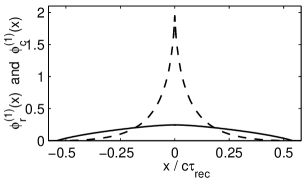
Figure 1: Green’s functions for the potentials $\phi_{r}$ (solid) and $\phi_{c}$ (dashed) at the time of recombination $\tau_{\rm rec}\simeq 2.15\,\tau_{e}$ with $\Omega_{\rm m}=0.35$, $\Omega_{\Lambda}=0.65$, $\Omega_{b}h^{2}=0.02$, and $h=0.65$.

The original delta function perturbation has separated into left-going and right-going waves, whose evolution spreads $\phi_{r}^{(1)}$ over space and diminishes the magnitude of the radiation disturbance. The gravitational potential hill of the radiation causes outward-directed gravitational forces which expel the CDM away from $x=0$. Three snapshots of the time evolution of $\phi_{r}^{(1)}$ and $\phi_{c}^{(1)}$ are shown in Fig. 2. Only the range $x>0$ needs to be calculated since the potential Green’s functions are even functions of $x$.

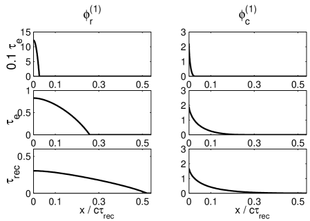
Figure 2: Time evolution of the Green’s functions of Fig. 1 describing the gravitational potentials for radiation (left) and CDM (right). The plots, from top to bottom, correspond to the conformal time values $0.1\,\tau_{e}$, $\tau_{e}$, and $\tau_{\rm rec}\simeq 2.15\,\tau_{e}$.

The Green’s functions are identically zero beyond the acoustic horizon, $|x|>S(\tau)$, where

$$S(\tau) \equiv \int_{0}^{\tau}c_{s}(\tau^{\prime})\,d\tau^{\prime}=$$

$$= \frac{4\tau_{e}}{3\sqrt{\beta}}\ln\left(\frac{\sqrt{1+\frac{3}{4}y\beta}+\tau_{e}\dot{y}\sqrt{\frac{3}{4}\beta}}{1+\sqrt{\frac{3}{4}\beta}}\right)$$

($S(\tau)\simeq\tau/\sqrt{3}$ when $\tau\ll\tau_{e}$). In a more careful treatment one will find weak precursors extending beyond the Green’s functions acoustic fronts up to the particle horizon $x=\pm c\tau$. The precursors arise because of partial photon, and in a full treatment neutrino, free streaming with the speed of light. Postponing detailed discussion of the photon diffusion until Sec. VI and of the neutrino free streaming until a separate paper, we continue the analysis of perturbation dynamics in the perfect fluid model.

The density and velocity perturbations of the photon-baryon and CDM fluids are determined from the $\phi_{r}$ and $\phi_{c}$ potentials by eqs. (46). The corresponding Green’s functions are plotted in Figs. 3 and 4. Characteristic features in the density and velocity Green’s functions and their connection to cosmological parameters are discussed in subsection IV.4. The delta function spikes at the acoustic wavefronts of $\delta_{r}^{(1)}$ and $v_{r}^{(1)}$ in the fluid model are fully calculable analytically and are considered in subsection IV.2.

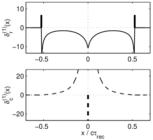
Figure 3: Green’s functions of the radiation density enhancement $\delta_{r}$ (top) and the CDM density enhancement $\delta_{c}$ (bottom) at the time of recombination. The vertical spikes represent the delta-function singularities of $\delta_{r}(x)$ at its wavefronts and of $\delta_{c}(x)$ at the origin.

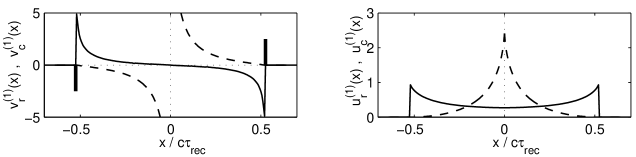
Figure 4: Green’s functions of the velocities $v_{r,c}\,{=}\,{-}\,\nabla u_{r,c}$ (left) and of the velocity potentials $u_{r,c}$ (right) at the time of recombination. Solid and dashed lines are for the radiation and CDM respectively.

IV.1 Sum rules

Sum rules are simple, easy to apply integral relations that offer a powerful tool for checking analytical formulae or numerical calculations. The sum rules are more general than the fluid approximation: they hold in the linear regime regardless of how complicated the internal dynamics of perturbations may be. They offer a simple method for estimating the accuracy of numerical calculations of the Green’s functions. In addition, the sum rules give insight into the connection between the position and Fourier space descriptions. They become indispensable for setting the initial conditions of Green’s functions when one considers perturbations to the full phase space distributions, Ref. Bashinsky (2001).

The idea of the sum rules is to use eq. (53) with $k=0$:

$$\phi^{(T)}(k\,{=}\,0,\tau)=\int^{+\infty}_{-\infty}dx\,\phi^{(1)}(x,\tau)~{}.$$ (62)

The time evolution of the $k=0$ Fourier modes, the magnitude of which we denote by upper case letters, e.g. $\phi^{(T)}(k\,{=}0,\tau)\equiv\Phi(\tau)$, satisfies easily solvable ordinary differential equations. The $k$-space equations at $k\,{=}\,0$ are especially simple because, given the adiabatic initial conditions, all the parameters characterizing relative motion of different matter and radiation components are unperturbed at all time on infinitely large scales. For example, in our case of the radiation-CDM model,

$$\Sigma(\tau)\equiv\int dx\,\sigma^{(1)}(x,\tau)=0.$$ (63)

Trivially integrating first of eqs. (27) over $x$ from $-\infty$ to $\infty$, we obtain the equation for the gravitational potential in the $k=0$ mode:

$$\ddot{\Phi}+3\left(1+c_{w}^{2}\right)\frac{\dot{y}}{y}\,\dot{\Phi}+\frac{3c_{w}^{2}}{4\tau_{e}^{2}y}\,\Phi=0~{}.$$ (64)

With $c_{w}$ given by eq. (22), the linear independent solutions of this equation are

$$f_{1} = 1+\frac{2}{9y}-\frac{8}{9y^{2}}-\frac{16}{9y^{3}}~{},$$

$$f_{2} = \frac{\sqrt{1+y}}{y^{3}}\simeq O(y)+\frac{1}{16}-\frac{1}{8y}+\frac{1}{2y^{2}}+\frac{1}{y^{3}}~{}.$$

Taking the linear combination of $f_{1}$ and $f_{2}$ satisfying the initial condition $\Phi(\tau\to 0)=1$, we obtain the sum rule for the gravitational potential:

$$\Phi(\tau)\equiv\int dx\,\phi^{(1)}(x,\tau)=\frac{9}{10}\,f_{1}+\frac{16}{10}\,f_{2}~{}.$$ (65)

The sum rules for $\phi_{r}$ and $\phi_{c}$ then follow immediately from eqs.(33,65,63):

$$\Phi_{r}\equiv\int dx\,\phi_{r}^{(1)}(x,\tau) = \frac{c_{w}^{2}}{c_{s}^{2}}\,\Phi~{},$$ (66a)

$$\Phi_{c}\equiv\int dx\,\phi_{c}^{(1)}(x,\tau) = \left(1-\frac{c_{w}^{2}}{c_{s}^{2}}\right)\Phi~{}.$$ (66b)

The sum rules for the radiation velocity potential $u_{r}$ and the combination $\frac{1}{4}\,\delta_{r}\,{+}\,\phi$ are relevant for CMB temperature anisotropy. The first sum rule simply follows from the first of eqs. (46h) and from eq. (66a):

$$U_{r}\equiv\int dx\,u_{r}^{(1)}(x,\tau) = \frac{3c_{w}^{2}\tau_{e}^{2}y}{2}\left(y\Phi\right)\dot{\vphantom{l}}~{}.$$ (67)

The second can be derived starting from eq. (48) and applying formulas of this subsection, including eq. (64),

$$\frac{1}{4}\,\Delta_{r}+\Phi \equiv \int dx\left(\frac{1}{4}\,\delta_{r}^{(1)}+\phi^{(1)}\right)=$$ (68)

$$= \dot{U}_{r}=-\,\frac{3c_{w}^{2}\tau_{e}^{2}y^{2}}{2}\left(\frac{\dot{y}}{y}\,\Phi\right)\dot{\vphantom{\frac{w}{w}}}~{}.$$

Finally, we give the sum rules for the radiation and CDM energy density enhancements. They follow from eqs. (46b–46e) and the second of eqs. (41):

$$\Delta_{r}=\frac{4}{3}\,\Delta_{c}=-\,\frac{2\tau_{e}^{2}\dot{y}}{A}\,\left(y\Phi\right)\dot{\vphantom{l}}~{},$$ (69)

with $\Delta_{r}\equiv\int dx\,\delta_{r}^{(1)}$ and $\Delta_{c}\equiv\int dx\,\delta_{c}^{(1)}$.

IV.2 Wavefront singularities

We can obtain exact analytic formulae describing Green’s functions at the acoustic wavefronts $|x|=S(\tau)$ in the fluid model. As one will see below, the wavefront spikes in the density and velocity Green’s functions play a significant role in the acoustic dynamics. For the wavefront analysis, it is convenient to factor the radiation potential as

$$\phi_{r}(x,\tau)=C(\tau)\,d(S(\tau)-|x|,\tau)$$ (70)

where for the perfect fluids, with $x^{\prime}\equiv S(\tau)-|x|$,

$$d(x^{\prime}\leq 0,\tau)\equiv 0~{},\quad\frac{\partial}{\partial x^{\prime}}\,d(+0,\tau)\equiv 1~{},$$ (71)

i.e. $d(x^{\prime},\tau)\simeq x^{\prime}\theta(x^{\prime})$ as $x^{\prime}\to 0$. Substituting these equations in eq. (34a), setting $|x|=S(\tau)$, and taking into account that at the wave fronts

$$\phi_{r}^{(1)}=\phi_{c}^{(1)}=0~{},\quad\dot{\phi}_{c}^{(1)}=0~{},$$ (72)

we find the following simple relation for $C(\tau)$:

$$2\dot{C}+\left(4\,\frac{\dot{y}}{y}+3\,\frac{\dot{c}_{s}}{c_{s}}\right)C=0~{}.$$ (73)

Here we have applied the formula

$$3c_{s}^{2}\,\frac{\dot{y}}{y}=\frac{\dot{y}}{y}+2\,\frac{\dot{c}_{s}}{c_{s}}$$

for the sound speed given by eq. (21). Integrating eq. (73) and normalizing the result to agree with the radiation era solution (58a) in the $y\to 0$ limit, we obtain:

$$C(\tau)=\frac{9~{}~{}}{2\tau_{e}^{2}y^{2}\left(3c_{s}^{2}\right)^{3/4}}~{}.$$ (74)

In particular, at $x=\pm S(\tau)$,

$$\dot{\phi}_{r}^{(1)}=\mp c_{s}\phi_{r}^{{}^{\prime}(1)}=\frac{3\sqrt{3}~{}~{}}{2\tau_{e}^{2}y^{2}\left(3c_{s}^{2}\right)^{1/4}}~{}.$$ (75)

The values of velocity potentials at the wave fronts follow from eqs. (46h):

$$u^{(1)}_{r}=\frac{3\sqrt{3}}{4}\left(3c_{s}^{2}\right)^{3/4}~{},~{}~{}~{}u^{(1)}_{c}=0~{}.$$ (76)

Because $\phi_{r}$ and $u_{r}$ are identically zero when $|x|>S(\tau)$, the velocity $v_{r}=-\nabla u_{r}$ and the radiation density $\delta_{r}$, given by eqs. (46b–46e), both contain a delta function singularity at the acoustic horizon:

$$\delta^{(1)}_{r,\rm~{}sing}=\epsilon^{(1)}_{r,\rm~{}sing}=3\left(3c_{s}^{2}\right)^{1/4}\delta_{\rm D}(\,|x|-S)~{},~{}~{}\,$$ (77a)

$$v^{(1)}_{r,\rm~{}sing}=\frac{3\sqrt{3}}{4}\left(3c_{s}^{2}\right)^{3/4}\mathop{\rm sign}(x)\,\delta_{\rm D}(\,|x|-S)~{}.~{}$$ (77b)

The dynamics of the shock-like singularities in the Green’s functions is linear, even if nonlinear effects would take place in the propagation of a real shock wave in the photon-baryon plasma. Indeed, the actual cosmological perturbations are the convolutions of the Green’s functions with the smooth primordial potential field. As long as the overall perturbations are small, they remain as regular as the primordial perturbation field and their dynamics is well in the linear regime. (On very small scales, there may exist physically relevant nonlinear effects, Ref. non , unrelated to the above Green’s function singularities. These effects are absent when photons and baryons are tightly coupled.)

IV.3 Numerical integration

From the hyperbolic (wave) nature of eqs. (34), the values of the potentials $\phi_{r}$ and $\phi_{c}$ at a point $(x,\tau+\Delta\tau)$ are uniquely determined by their past values within the interval $[x-c_{s}\Delta\tau,x+c_{s}\Delta\tau]$ at time $\tau$. Cusps at the potential wavefronts will not be distorted by numerical errors during the evolution if discretization intervals in space and time are related so that $c_{s}\Delta\tau$ is a multiple of $\Delta x$. In particular, for $c_{s}\Delta\tau=\Delta x$, the second derivative terms in eqs. (34) may be approximated by the second order scheme

$$\ddot{\phi}_{r}(x,\tau)-c_{s}^{2}\nabla^{2}\phi_{r}(x,\tau)~{}\simeq$$

$$\qquad\simeq~{}\frac{1}{(\Delta\tau)^{2}}\,[\phi_{r}(x,\tau+\Delta\tau)+\phi_{r}(x,\tau-\Delta\tau)$$

$$\qquad\qquad~{}-~{}\phi_{r}(x+c_{s}\Delta\tau,\tau)-\phi_{r}(x-c_{s}\Delta\tau,\tau)]~{},\qquad$$ (78)

$$\ddot{\phi}_{c}(\tau)~{}\simeq$$

$$\qquad\simeq~{}\frac{1}{(\Delta\tau)^{2}}\left[\phi_{c}(\tau+\Delta\tau)+\phi_{c}(\tau-\Delta\tau)-2\phi_{c}(\tau)\right]~{}.$$

In practice, we use the horizon radius $S(\tau)$ for the time evolution coordinate and take $\Delta S=\Delta x$.

The first time derivatives of $\phi_{r}$ and $\phi_{c}$ can be approximated by an implicit second order scheme

$$\dot{\phi}(\tau)\simeq\frac{1}{\Delta\tau}\left[\phi(\tau+\Delta\tau)-\phi(\tau)\right]-\frac{\Delta\tau}{2}\,\ddot{\phi}(\tau)~{}.$$ (79)

An explicit scheme should be avoided as numerically unstable. With the substitutions (78–79), eqs. (34) become finite difference equations that can be straightforwardly solved for the values of $\phi_{r}$ and $\phi_{c}$ at $(x,\tau+\Delta\tau)$. The resulting finite difference scheme is of the second order and it preserves the form of cusps or discontinuities in propagating waves.

We start the integration from the radiation era solutions (58b) at some small initial time, e.g. $\tau_{\rm init}\simeq 10^{-4}\tau_{e}$. To follow the evolution over a large dynamic range, the spacings of the space and time grids are increased by a factor of $2$ every time the extent of the acoustic horizon $S$ doubles. Then the number of discretization points $N=S/\Delta x$ used to represent the Green’s functions at all later times remains in the range $N_{\rm min}\leq N\leq 2N_{\rm min}$ where $N_{\rm min}$ is the initial number of points within the horizon. The total number of $\phi_{r}$ and $\phi_{c}$ evaluations needed to evolve the potentials to a final time $\tau_{\rm fin}$ is of the order of $N^{2}\ln(\tau_{\rm fin}/\tau_{\rm init})$.

Whenever a Fourier space transfer function is needed, it can be obtained from the corresponding Green’s function using the Fast Fourier Transform (FFT) algorithm. The FFT can be efficiently applied to Fourier integrals as described in Ref. Press et al. (1992) with its CPU time scaling as $N\log_{2}N$. Due to the finite extent of the Green’s functions, the related transfer functions oscillate in $k$ and $\tau$ requiring in general a larger number of evaluations for their direct Fourier space calculation with the same accuracy.

The sum rules introduced in Subsection IV.1 prove to be a highly efficient debugging tool available for calculations in position space. The sum rule relations can also be used to estimate the numerical error of computations.

Calculations of the Green’s functions in Figs. 1 and 2 proceeded from $\tau_{\rm init}\simeq 10^{-4}\tau_{e}$ to $\tau_{\rm rec}\simeq 2.15\,\tau_{e}$. The corresponding CPU time for our Pentium IV PC is $0.04\,s$ with the minimal number of points in the spatial grid $N_{\rm min}=64$ and $0.1\,s$ with $N_{\rm min}=128$. The accuracy of these calculations as estimated by the sum rules is $0.19\%$ and $0.05\%$ respectively.

IV.4 Discussion of Green’s function features

The plane parallel Green’s functions for the potentials $\phi_{r}$ and $\phi_{c}$, plotted in Figs. 1 and 2, are continuous functions of $x$ and $\tau$. In the fluid approximation, the radiation potential is characterized by discontinuous first derivatives (kinks) at its acoustic wavefronts as described by eq. (75). The CDM potential has a central cusp reflecting the initial repulsive singularity in the gravitational potential $\phi_{r}^{(1)}$; this cusp is preserved because the CDM particles have no thermal motion. In fact, once the photon energy density becomes negligible in the matter dominated era, the potential $\phi_{c}(x,\tau)$ stops evolving, as may be seen from eqs. (34) in the limit $y\gg 1$.

The discontinuities in the potential derivatives give rise to delta function singularities in the corresponding density and velocity transfer functions, following from eqs. (46) and plotted for the time of recombination in Figs. 3 and 4. The singularities are visualized in the figures by the vertical spikes at $x=\pm S$ for $\delta_{r}$ and $v_{r}$ and at $x=0$ for $\delta_{c}$.

The wavefront singularities in $\delta_{r}^{(1)}(x)$ and $v_{r}^{(1)}(x)$ are described analytically by eqs. (77). Their significance in perturbation dynamics may be characterized by the delta function contributions to the sum rule integrals for the corresponding Green’s functions. For the radiation energy density, we find that in our $\Lambda$CDM model at recombination $\int dx\,\delta^{(1)}_{r}{}_{\rm sing}/\int dx\,\delta^{(1)}_{r}\simeq 2.7/(-2.3)$. Thus the delta function singularities play a major role in the perturbation dynamics even on the largest scales. Their relative contribution to the CMB anisotropy even increases on smaller scales because the oscillation amplitude of the delta function Fourier transform does not fall off with $k$, as opposed to the oscillations in the non-singular term Fourier transforms. We have shown in Ref. Bashinsky and Bertschinger (2001) that in real space the singularities give rise to a localized feature in the CMB angular correlation function $C(\theta)$.

The delta function singularities acquire a finite width when photon diffusion, or Silk damping, Ref. Silk (1968), is included into the analysis. When the photon mean free path is small compared with the scales considered, Silk damping can be approximated as

$$\delta^{(T)}_{r}(k)\simeq e^{-k^{2}x_{S}^{2}}\,\delta^{(T)}_{r~{}\rm fluid}(k)~{},$$ (80)

Refs. Peebles and Yu (1970); Weinberg (1971); Kaiser (1983). As found in Ref. Kaiser (1983),

$$x_{S}^{2}(\tau)\simeq\frac{1}{6}\int_{0}^{\tau}\left[1-\frac{14}{15}\left(3c_{s}^{2}\right)+\left(3c_{s}^{2}\right)^{2}\right]\frac{cd\tau}{an_{e}\sigma_{T}}~{}$$ (81)

where $n_{e}$ is the proper number density of electrons and $\sigma_{T}$ is Thomson scattering cross section. Silk damping broadens a delta function singularity in a position space Green’s function to a Gaussian of finite width:

$$\delta_{\rm D}(|x|-S)\to\frac{1}{2x_{S}\sqrt{\pi}}~{}\exp\left[-\,\frac{\left(|x|-S\right)^{2}}{4x_{S}^{2}}\right]~{},$$ (82)

as obtained by applying the filtering (80) to the constant Fourier transform of a delta function. We rederive eqs. (80–81) within our position space formalism in Sec. VI.

The CDM density perturbations, with the Green’s function shown in the bottom panel of Fig. 3, eventually seed the formation of galaxies. The central spike in the figure arises from $\nabla^{2}\phi_{c}$ in the second of eqs. (46e). It is negative because of the repulsive sign of the initial gravitational potential peak, as shown in the top row of Fig. 2. The spike is surrounded by positive tails because the CDM pushed out from $x=0$ piles up into the region between $x=0$ and the acoustic wavefront.

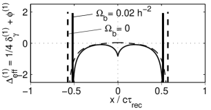
Figure 5: The position space transfer function for the intrinsic ($\frac{1}{4}\delta_{\gamma}$) plus gravitational redshift contributions to the CMB temperature anisotropy $\Delta T/T$ at recombination assuming tight coupling between photons and baryons. The values of cosmological parameters are taken as $\Omega_{\rm m}=0.35$, $\Omega_{\Lambda}=0.65$, and $h=0.65$. Baryon drag effects are evident from comparing the solid, $\Omega_{b}h^{2}=0.02$, and the dashed, $\Omega_{b}=0$, lines.

To understand the physics of the dip in $\delta_{r}^{(1)}(x)$ at $x=0$ in Fig. 3, let us examine the intrinsic radiation temperature perturbation $\delta_{r}/4$ corrected for the temperature redshift by the local metric perturbation at $x$:

$$\Delta_{\rm eff}\equiv\frac{1}{4}\,\delta_{r}+\phi~{}.$$ (83)

The plane-parallel Green’s function for $\Delta_{\rm eff}$ at recombination is shown in Fig. 5. The smoothness of $\Delta_{\rm eff}^{(1)}$ at $x=0$ in the absence of baryons (dashed line in Fig. 5) can be understood as the condition of thermodynamic, Ref. The , and hydrostatic photon equilibrium near $x=0$. (Obviously the equilibrium does not apply at the acoustic wavefronts, but it does hold as $x\to 0$ where the elapsed time is many sound-crossing times.) Linearizing the relativistic equation of hydrostatic equilibrium,

$$\nabla_{i}p+(\rho+p)\nabla_{i}\phi=0\ ,$$ (84)

for the case of the radiation fluid containing no baryons we obtain

$$\nabla_{i}\left({1\over 3}\,\delta_{\gamma}+{4\over 3}\,\phi\right)={4\over 3}\,\nabla_{i}\Delta_{\rm eff}=0\ .$$ (85)

Thus, if $\rho_{b}=0$, $\Delta_{\rm eff}$ has zero gradient in equilibrium. If $\Omega_{b}\neq 0$, on the other hand, the hydrostatic eq. (84) applied to tightly coupled radiation-baryon fluid gives $\nabla_{i}\Delta_{\rm eff}=-(3/4)\beta y\nabla_{i}\phi$. The positive cusp of the CDM gravitational potential becomes a dip of CMB temperature. The dip appears because the heavy pressureless baryons are repelled by the cusp in the CDM gravitational potential $\phi_{c}$ from the $x=0$ region and they drag the coupled photon fluid away from the origin. In eq. (48), rewritten as

$$\Delta_{\rm eff}=\dot{u}_{r}+\frac{3}{4}\,\beta\left(y\dot{u}_{r}+\dot{y}u_{r}-y\phi_{r}\right)-\frac{3}{4}\,\beta y\phi_{c}~{},$$ (86)

only the last, $\phi_{c}$, term on the right hand side has a cusp at $x=0$. The contribution of this term and thus the magnitude of the dip in $\Delta_{\rm eff}$ are roughly proportional to $\beta y(\tau_{\rm rec})\propto\Omega_{b}h^{2}$. Another effect of the baryonic constituent on the radiation perturbations evident from Fig. 5 is the decrease of the sound speed and thereby the reduction of the acoustic distance compared with a pure photon gas.

V Perturbation Dynamics Beyond the Fluid Model

Now we will distinguish between photon and baryon perturbations and will not assume the fluid approximation for photons. We will continue to exclude neutrino perturbations from our model as described in Sec. II.1.

The linear evolution equations for the photon and baryon velocity potentials follow from linearized Boltzmann equation and are given in the Appendix as the second of eqs. (150) and the second of eqs. (156). In these equations, the terms proportional to the inverse of the mean conformal time of a photon free flight,

$$\tau_{c}^{-1}\equiv{an_{e}\sigma_{T}}~{},$$ (87)

are due to Thomson scattering between photons and baryons. The Thomson scattering damps the velocity potential difference, for which we define

$$u_{d}\equiv u_{b}-u_{\gamma}~{}.$$ (88)

However, the scattering does not affect the overall momentum density of the plasma. Defining a momentum-averaged velocity potential of photons and baryons

$$u_{r}\equiv\frac{(\rho_{\gamma}+p_{\gamma})u_{\gamma}+\rho_{b}u_{b}}{(\rho_{\gamma}+p_{\gamma})+\rho_{b}}=\frac{1}{B}\left(u_{\gamma}+\frac{3\beta y}{4}\,u_{b}\right)~{},$$ (89)

where $B$ is given by eq. (35), from the velocity equations in eqs. (150, 156) we find:

$$\begin{array}[]{l}\dot{u}_{r}=\frac{1}{B}\left(\frac{1}{4}\,\delta_{\gamma}+\nabla^{2}\pi_{\gamma}-\frac{3\beta\dot{y}}{4}\,u_{r}\right)+\phi~{},\\ \dot{u}_{d}=-\frac{\dot{a}}{a}\left(u_{r}+\frac{1}{B}\,u_{d}\right)-\frac{1}{4}\,\delta_{\gamma}-\nabla^{2}\pi_{\gamma}-\frac{1}{\tau_{c}}\,\frac{4B}{3\beta y}\,u_{d}~{}.\end{array}$$ (92)

Substituting $u_{\gamma}=u_{r}-\frac{3\beta y}{4B}\,u_{d}$ and $u_{b}=\frac{1}{B}\,u_{d}+u_{r}$ in the density evolution equations in eqs. (150, 156), and defining

$$\delta_{d}\equiv\delta_{b}-\frac{3}{4}\,\delta_{\gamma}~{},$$ (93)

we obtain

$$\begin{array}[]{l}\dot{\delta}_{\gamma}=\frac{4}{3}\,\nabla^{2}\left(u_{r}-\frac{3\beta y}{4B}\,u_{d}\right)+4\dot{\psi}~{},\\ \dot{\delta}_{d}=\nabla^{2}u_{d}~{}.\end{array}$$ (96)

The cold dark matter density and velocity perturbations evolve as

$$\begin{array}[]{l}\dot{\delta}_{c}=\nabla^{2}u_{c}+3\dot{\psi}~{},\\ \dot{u}_{c}=-\frac{\dot{a}}{a}\,u_{c}+\phi~{}.\end{array}$$ (99)

The conformal Newtonian gauge potentials $\phi$ and $\psi$, defined by eq. (8), can be determined non-dynamically from the first, second, and fourth relations of eqs. (136):

$$\nabla^{2}\psi=\frac{3}{2\tau_{e}^{2}y}\left[\frac{B}{y}\,\delta_{\gamma}+(1-\beta)\delta_{c}+\beta\delta_{d}+3\frac{\dot{y}}{y}\,u\right]\,,~{}$$ (100a)

$$\psi-\phi=\frac{6}{\tau_{e}^{2}y^{2}}\,\pi_{\gamma}~{},\qquad\qquad\qquad\qquad\qquad\qquad\quad$$ (100b)

where formula (19) was applied. The variable $u$ in eq. (100a) is defined as previously by eq. (36).

Two independent variables are needed to describe the species number density perturbations $\frac{3}{4}\delta_{\gamma}$, $\delta_{b}$, and $\delta_{c}$ relative to each other. For one such variable we use a potential generating the baryon density perturbation relatively to photons:

$$\nabla^{2}\sigma_{d}\equiv\frac{3}{2\tau_{e}^{2}}\,\delta\left(\ln\frac{\rho_{b}}{T^{3}_{\gamma}}\right)=\frac{3}{2\tau_{e}^{2}}\,\delta_{d}~{}.$$ (101)

The other can be the entropy potential $\sigma$ from eqs. (24, 23) that now equals

$$\nabla^{2}\sigma \equiv \frac{3}{2\tau_{e}^{2}}\,\delta\left(\ln\frac{T^{3}_{\gamma}}{\rho_{\rm m}}\right)=$$ (102)

$$= \frac{3}{2\tau_{e}^{2}}\left[(1-\beta)\left(\frac{3}{4}\,\delta_{\gamma}-\delta_{c}\right)-\beta\delta_{d}\right].$$

The time derivatives of $\nabla^{2}\sigma_{d}$ or $\nabla^{2}\sigma$ equal a full $\nabla^{2}$ of a certain linear combination of velocity potentials $u_{a}$. Differentiating both sides of eq. (101) and eq. (102) with respect to $\tau$, remembering eqs. (96–99), and lifting $\nabla^{2}$, one obtains:

$$\begin{array}[]{l}\dot{\sigma}=\frac{3}{2\tau_{e}^{2}}\left[(1-\beta)\left(u_{r}-u_{c}\right)-\frac{\beta A}{B}\,u_{d}\right]~{},\\ \dot{\sigma}_{d}=\frac{3}{2\tau_{e}^{2}}\,u_{d}~{}.\end{array}$$ (105)

Taking another time derivative of both sides of eqs. (105), using the dynamical $\dot{u}_{a}$ equations from eqs. (92, 99), and expressing all the resulting density and velocity perturbations in terms of $\nabla^{2}\psi$, as given by eq. (100a), $\nabla^{2}\sigma_{a}$, eqs. (101, 102), and $\dot{\sigma}_{a}$, eqs. (105),

$$\ddot{\sigma}+\frac{\beta c_{s}^{2}}{c_{w}^{2}}\,\ddot{\sigma}_{d}+\left(1+3c_{w}^{2}-3c_{s}^{2}\right)\frac{\dot{y}}{y}\,\dot{\sigma}+\frac{\beta c_{s}^{2}}{c_{w}^{2}}\,\frac{\dot{y}}{y}\,\dot{\sigma}_{d}=y\left(c_{s}^{2}-c_{w}^{2}\right)\nabla^{2}\left(\psi+\frac{\sigma}{y}+\frac{2\pi_{\gamma}}{c_{w}^{2}\tau_{e}^{2}y^{2}}\right)\,,$$ (106a)

$$\ddot{\sigma}_{d}+\left(\frac{4}{9\beta yc_{s}^{2}\tau_{c}}+\frac{\dot{y}}{y}\right)\dot{\sigma}_{d}+\frac{9\dot{y}c_{w}^{2}}{4}\,\dot{\sigma}=-\,\frac{3c_{w}^{2}y^{2}}{4}\nabla^{2}\left(\psi+\frac{\sigma}{y}+\frac{2\pi_{\gamma}}{c_{w}^{2}\tau_{e}^{2}y^{2}}\right)\,.$$ (106b)

Similarly to the fluid case, these equations are supplemented by the formula following from the first line of eq. (23), eqs. (24, 20), and the Einstein equations (136):

$$\ddot{\psi}+\left(3c_{w}^{2}+2\right)\frac{\dot{y}}{y}\,\dot{\psi}+\frac{\dot{y}}{y}\,\dot{\phi}+\frac{3c_{w}^{2}}{4\tau_{e}^{2}y}\,\phi=c_{w}^{2}\nabla^{2}\left(\psi+\frac{\sigma}{y}+\frac{2\pi_{\gamma}}{c_{w}^{2}\tau_{e}^{2}y^{2}}\right)~{}.$$ (106c)

Here $\phi$ is expressed via $\psi$ and $\pi_{\gamma}$ using eq. (100b). The set of eqs. (106, 100b) is not closed as long as $\pi_{\gamma}$ remains an independent variable.

We split the total potential $\psi$ into potentials $\psi_{a}$ generated by the individual species:

$$\psi=\psi_{\gamma}+\psi_{c}+\psi_{d}~{}.$$ (107)

The dynamics of the potentials $\psi_{a}$ may be described by coupled wave equations provided the decomposition (107) is performed according to the two following requirements: First, on small scales, when the velocity term in eq. (100a) is negligible, every $\nabla^{2}\psi_{a}$ is proportional to the corresponding $\delta_{a}$ and is independent of the density of the other species. Second, the potentials $\psi_{a}$ are given by linear combinations of $\psi$ and the entropy potentials $\sigma$ and $\sigma_{d}$. These linear combinations are unique and are easily found to be

$$\psi_{\gamma} = \frac{c_{w}^{2}}{c_{s}^{2}}\left(\psi+\frac{\sigma}{y}\,\right)~{},$$ (108a)

$$\psi_{c} = \left(1-\frac{c_{w}^{2}}{c_{s}^{2}}\right)\psi-\left(\frac{c_{w}^{2}}{c_{s}^{2}}\right)\frac{\sigma}{y}-\frac{\beta\sigma_{d}}{y}~{},$$ (108b)

$$\psi_{d} = \frac{\beta\sigma_{d}}{y}\vphantom{\frac{c_{w}^{2}}{c_{s}^{2}}}~{}.$$ (108c)

The corresponding Laplacians are

$$\nabla^{2}\psi_{\gamma} = \frac{3}{2\tau_{e}^{2}y}\left(\frac{B}{y}\,\delta_{\gamma}+\frac{B}{A}\,3\,\frac{\dot{y}}{y}\,u\right),$$ (109a)

$$\nabla^{2}\psi_{c} = \frac{3}{2\tau_{e}^{2}y}\left[(1-\beta)\delta_{c}+\left(1-\frac{B}{A}\right)3\,\frac{\dot{y}}{y}\,u\right],~{}~{}$$ (109b)

$$\nabla^{2}\psi_{d} = \frac{3}{2\tau_{e}^{2}y}\left(\beta\delta_{d}\vphantom{\frac{B}{A}}\right).$$ (109c)

The evolution equations for the potentials $\psi_{a}$ are obtained by substituting eq. (107) and

$$\sigma=y\left[\left(\frac{c_{s}^{2}}{c_{w}^{2}}-1\right)\psi_{\gamma}-\psi_{c}-\psi_{d}\right],~{}~{}\sigma_{d}=y\,\frac{1}{\beta}\,\psi_{d}$$ (110)

in eqs. (106, 100b). Upon the substitution, one finds a system of coupled second order wave equations generalizing eqs. (34). For simplicity, here we write these equations omitting the terms with no or only first derivatives of the potentials $\psi_{a}$ and $\pi_{\gamma}$ unless a term contains the large damping parameter $\tau_{c}^{-1}$. The neglected terms contribute only to the dynamics on large scales $\lambda\gtrsim\tau$, when the fluid eqs. (34) can be used. With the remaining terms, one obtains that on scales $\lambda\ll\tau$

$$\ddot{\psi}_{\gamma}+\ddot{\psi}_{d} \approx c_{s}^{2}\,\nabla^{2}\left(\psi_{\gamma}+\frac{2\pi_{\gamma}}{c_{s}^{2}\tau_{e}^{2}y^{2}}\right)\,,$$ (111a)

$$\ddot{\psi}_{d}+\frac{4}{9\beta yc_{s}^{2}\tau_{c}}\,\dot{\psi}_{d} \approx -\,\frac{3\beta yc_{s}^{2}}{4}\,\nabla^{2}\left(\psi_{\gamma}+\frac{2\pi_{\gamma}}{c_{s}^{2}\tau_{e}^{2}y^{2}}\right),~{}~{}~{}~{}~{}\,$$ (111b)

$$\ddot{\psi}_{c} \approx 0~{}.$$ (111c)

In general, eqs. (111) should be completed by the evolution equations for the higher multipoles of the radiation phase space density $f_{\gamma\,l\geq 2}$ and polarization multipoles $g_{\gamma\,l}$ that are given in the Appendix. However, in the following section we find that in the next to the leading order in the photon-baryon coupling $\tau_{c}$, $\pi_{\gamma}\equiv\frac{1}{2}\,f_{\gamma\,2}$ is fully determined by $\psi_{\gamma}$ and $\dot{\psi}_{\gamma}$. Then, neglecting special features of neutrino dynamics, the above equations provide a closed system.

VI Tight coupling: Next to the leading order

Now we can consider systematically how the general formulae of the previous section reduce to the fluid equations in the limit of tight photon-baryon coupling and find the $O(\tau_{c})$ leading corrections to the fluid approximation.

First of all, $\dot{u}_{d}$ equation in eqs. (92) and all the equations for $\dot{f}_{\gamma\,l\geq 2}$ and $\dot{g}_{\gamma\,l}$ in the Appendix have the generic form

$$\dot{f}_{l}=a-\frac{1}{r\tau_{c}}\left(f_{l}-b\right)~{},$$ (112)

where $r$ is a positive number and $a$ and $b$ are some linear combinations of variables other than $f_{l}$. In the tight coupling regime, $\tau_{c}\ll\tau$, the evolution given by eq. (112) will quickly, over a time of order $\tau_{c}$, drive $f_{l}$ to $f_{l}\simeq b+r\tau_{c}(a-\dot{b})$, as is evident from the explicit solution of eq. (112)

$$\begin{array}[]{rcl}f_{l}&=&b+\int^{\tau}d\tau^{\prime}\,(a-\dot{b})\,\exp\left(-\int^{\tau}_{\tau^{\prime}}\frac{d\tau^{\prime\prime}}{r\tau_{c}}\right)=\\ &=&b+r\tau_{c}(a-\dot{b})+O(\tau_{c}^{2})~{}.\end{array}$$ (115)

Thus at tight coupling the dynamical equations of the form (112) reduce to algebraic equations $f_{l}\simeq b$ up to $O(\tau_{c}^{0})$ or, if $b$ in eq. (112) is absent, $f_{l}\simeq r\tau_{c}a$ up to $O(\tau_{c})$.

Applying this observation to the evolution of the photon polarization averaged multipoles $f_{\gamma\,l}$ in eqs. (150) and to the polarization difference multipoles $g_{\gamma\,l}$ in eqs. (155), we see that each $l\geq 3$ multipole is suppressed relative to the corresponding lower multipole by an extra power of $\tau_{c}$ . Since $f_{\gamma\,1}=\frac{4}{3}\,u_{\gamma}\sim\tau_{c}^{0}$, we then find that $f_{\gamma}{}_{l}\sim\tau_{c}^{l-1}$ for $l\geq 1$, $\tilde{g}_{\gamma}{}_{0}\sim\tau_{c}$, $\tilde{g}_{\gamma}{}_{1}\sim\tau_{c}^{2}$, and $g_{\gamma}{}_{l}\sim\tau_{c}^{l-1}$ for $l\geq 2$. The equations for $\dot{f}_{\gamma\,2}$, $\dot{\tilde{g}}_{\gamma\,0}$ and $\dot{g}_{\gamma\,2}$ reduce to the following algebraic relations:

$$f_{\gamma\,2}\simeq\frac{1}{10}\left(f_{\gamma\,2}+{\tilde{g}}_{\gamma\,0}+g_{\gamma\,2}\right)+\tau_{c}\,\frac{2}{5}\,f_{\gamma\,1}~{},\qquad$$

$${\tilde{g}}_{\gamma\,0}\simeq\frac{1}{2}\left(f_{\gamma\,2}+{\tilde{g}}_{\gamma\,0}+g_{\gamma\,2}\right)~{},$$ (116)

$$g_{\gamma\,2}\simeq\frac{1}{10}\left(f_{\gamma\,2}+{\tilde{g}}_{\gamma\,0}+g_{\gamma\,2}\right)~{}$$

where the omitted terms are $O(\tau_{c}^{2})$. Similarly, from the second of eqs. (92),

$$u_{d}\simeq-\tau_{c}\,\frac{3\beta y}{4B}\left(\frac{1}{4}\,\delta_{\gamma}+\frac{\dot{y}}{y}\,u_{r}\right)~{}.$$ (117)

Resolving the linear algebraic system (116) in terms of $f_{\gamma\,1}$ and then remembering eq. (117) we find:

$$\pi_{\gamma}\equiv\frac{1}{2}\,f_{\gamma\,2}\simeq\tau_{c}\,\frac{4}{15}\,f_{\gamma\,1}\equiv\tau_{c}\,\frac{16}{45}\,u_{\gamma}\simeq\tau_{c}\,\frac{16}{45}\,u_{r}~{}.$$ (118)

Substitution of results (117, 118) into the right hand side of $\dot{\delta}_{\gamma}$ and $\dot{u}_{r}$ equations in eqs. (96, 92) gives

$$\begin{array}[]{l}\dot{\delta}_{\gamma}\simeq\frac{4}{3}\left[1+\tau_{c}\left(\frac{3\beta y}{4B}\right)^{2}\frac{\dot{y}}{y}\right]\nabla^{2}u_{r}+\frac{1}{3}\,\tau_{c}\left(\frac{3\beta y}{4B}\right)^{2}\nabla^{2}\delta_{\gamma}+4\dot{\psi}~{},\\ \dot{u}_{r}\simeq\frac{1}{B}\left(\frac{1}{4}\,\delta_{\gamma}-\frac{3\beta\dot{y}}{4}\,u_{r}+\tau_{c}\,\frac{16}{45}\,\nabla^{2}u_{r}\right)+\phi~{}.\end{array}$$ (121)

Comparing these equations with their perfect fluid analogues, eqs. (15c–15d), one can identify two qualitatively new terms appearing in the $O(\tau_{c})$ order. The $\nabla^{2}\delta_{\gamma}$ term in the first equation corresponds phenomenologically to heat conduction and $\nabla^{2}u_{r}$ in the second to bulk viscosity of adiabatic scalar perturbations in the photon-baryon plasma.

If Thomson scattering did not partially polarize the scattered radiation, in place of eqs. (116) we would find $f_{\gamma\,2}\simeq\tau_{c}\,\frac{2}{5}\,f_{\gamma\,1}$. This is $25\%$ less than the result (118) and would wrongly yield a $25\%$ smaller value of the radiation bulk viscosity. The relevance of fluctuations in photon polarization for dissipation of the perturbations in photon-baryon fluid was pointed out in Ref. Kaiser (1983).

The remaining undetermined quantity describing the relative motion of photons and baryons is their number density difference $\delta_{d}$, which enters the Poisson equation (100a). We will calculate the related potential $\sigma_{d}$ defined by eq. (101). Within the $O(\tau_{c})$ accuracy considered here one can substitute the perfect fluid expressions (46) into the right hand side of eq. (117). Then replacing $\phi_{r}$ and $\phi_{c}$ by $\phi$ and $\sigma$ and using the second of eqs. (27) to eliminate $\nabla^{2}\left(\phi+\sigma/y\right)$, we find

$$u_{d}\simeq-\,\tau_{c}\,\frac{2\tau_{e}^{2}}{3}\,\frac{3\beta}{4(1-\beta)}\left(y\dot{\sigma}\right)\dot{\vphantom{l}}~{}.$$ (122)

The relation $\dot{\sigma}_{d}=3/(2\tau_{e}^{2})u_{d}$ from eq. (105) can then be integrated from $\tau=0$, with $\left.\sigma_{d}\right|_{\tau=0}=0$ for adiabatic perturbations, to a given $\tau$:

$$\sigma_{d}\simeq-\,\tau_{c}\,\frac{3\beta}{4(1-\beta)}\,y\dot{\sigma}~{}.$$ (123)

Thus to first order in $\tau_{c}$ one can continue to describe the perturbation dynamics by only two independent fields $\phi_{r}\equiv\psi_{\gamma}$ and $\phi_{c}\equiv\psi_{c}$. By eqs. (108, 100b), these fields reduce to our earlier definitions (33) in $\tau_{c}\to 0$ limit. In the $O(\tau_{c})$ order, the potential $\psi_{d}$ is related to $\phi_{r}$ and $\phi_{c}$ via eq. (108c) and eq. (123), in which $\sigma$ may be substituted by the $O(\tau_{c}^{0})$ order expression (32).

Since $\pi_{\gamma}$ in eq. (118) is an $O(\tau_{c})$ quantity, $u_{r}$ on the right hand side of eq. (118) may also be expressed in terms of $\phi_{r}$ using the leading order relations (46h). When the corresponding expression for $\pi_{\gamma}$ and eq. (123) are used to close the dynamical equations of the previous subsection, one finds two coupled differential equations for $\phi_{r}$ and $\phi_{c}$ that contain all the terms of eqs. (34) and additional terms proportional to $\tau_{c}$. (Note that the third time derivative of $\sigma$ arising from $\ddot{\sigma}_{d}$ may be reduced within our $O(\tau_{c})$ accuracy by relations (27) to terms containing a lesser number of time derivatives.) When $\tau_{c}\ll\tau$, the $O(\tau_{c})$ terms containing three derivatives of the potential may still contribute appreciably to small scale variations of the potentials when their higher $\tau$ or spatial derivatives become increasingly large. Retaining only the second derivative terms with $O(\tau_{c}^{0})$ coefficients and all the third derivative terms, from eqs. (111a, 111c) we arrive at the following system, valid on small scales $\lambda\ll\tau$:

$$\ddot{\phi}_{r} \simeq c_{s}^{2}\,\nabla^{2}\phi_{r}+2\tau_{c}g\,\nabla^{2}\dot{\phi}_{r}\,,\qquad$$ (124a)

$$\ddot{\phi}_{c} \simeq 0$$ (124b)

where

$$g(\tau)\equiv\frac{1}{6}\left(1-\frac{14}{15B}+\frac{1}{B^{2}}\right)\,.$$ (125)

The last term in eq. (124a) and so the expression (125) receive contributions from both $\ddot{\psi}_{d}$ and $\pi_{\gamma}$ terms in eq. (111a).

The $\nabla^{2}\dot{\phi}_{r}$ term in eq. (124a) describes the famous Silk damping of perturbations in the photon-baryon plasma on small scales, Ref. Silk (1968). In momentum space, the dispersion relation imposed by eq. (124a) on a plane wave $\phi_{r}=A_{r}\exp{(i{\bf k}\cdot{\bf r}-i\omega\tau)}$ is

$$\omega^{2}+2i\tau_{c}gk^{2}\omega-k^{2}c_{s}^{2}=0~{}.$$ (126)

The solutions to first order in $\tau_{c}$ are $\omega=\pm\,kc_{s}-i\gamma$ with the damping rate

$$\gamma\simeq\tau_{c}gk^{2}~{}.$$ (127)

This rate coincides with the result of Ref. Kaiser (1983), where derivations were done with a different approach that also took into account the polarizing property of Thomson scattering.

One can quantitatively describe photon diffusion at the sharp wavefront of $\phi_{r}^{(1)}(x,\tau)$, as it evolves from $\tau_{\rm init}\to 0$ to a certain finite $\tau$, by considering the full eq. (34a) with the third derivative term $2\tau_{c}g\nabla^{2}\dot{\phi}_{r}$ added to its right hand side. We look for a solution in the wavefront region $\left|S(\tau)-|x|\right|\ll\tau$ using the ansatz (70):

$$\phi_{r}^{(1)}=C(\tau)\,d(x^{\prime},\tau)~{},\quad x^{\prime}\equiv S(\tau)-|x|~{}$$

where $C(\tau)$ is given by eq. (74) and initially $d(x^{\prime},0)\approx x^{\prime}\theta(x^{\prime})$. Assuming that

$$\left|{\partial d}/{\partial x^{\prime}}\right|\gg\left|d/\tau\right|~{}~{}\mbox{and}~{}~{}\left|{\partial d}/{\partial x^{\prime}}\right|\gg\left|{\partial d}/{\partial\tau}\right|~{}$$ (128)

and remembering eq. (73) as the condition of cancellation of the ${\partial d}/{\partial x^{\prime}}$ terms, we find:

$$\frac{\partial^{2}d}{\partial x^{\prime}\partial\tau}\simeq\tau_{c}g\,\frac{\partial^{3}d}{\partial x^{\prime}{}^{3}}~{}.$$

Integrating over $dx^{\prime}$ from $-\infty$ to a given $x^{\prime}$, we arrive at the classical diffusion equation

$$\frac{\partial d}{\partial\tau}\simeq\tau_{c}g\frac{\partial^{2}d}{\partial x^{\prime}{}^{2}}~{}.$$ (129)

The solution of this equation satisfies the second condition in eq. (128) provided $\tau_{c}$ is much less than the characteristic scale over which $d(x^{\prime},\tau)$ varies in $x^{\prime}$. Individual Fourier modes of any function satisfying eq. (129) are damped as

$$d(k,\tau)\simeq e^{-k^{2}x_{S}^{2}(\tau)}d(k,0)$$ (130)

where

$$x_{S}^{2}(\tau)=\int_{0}^{\tau}g(\tau^{\prime})\,\tau_{c}(\tau^{\prime})\,d\tau^{\prime}~{},$$ (131)

in agreement with eqs. (80–81).

By eq. (124b), small scale CDM dynamics is not affected by Silk damping.

VII Conclusions

We have shown how to reduce the linearized cosmological dynamics of gravitationally interacting species in the conformal Newtonian gauge to a system of coupled wave equations. These equations indicate that the linear evolution of not only the density fluctuations but also of the corresponding gravitational potentials (metric perturbations) proceeds causally and locally, as opposed to the instantaneous action at a distance seemingly implied by the Poisson equation. In the fluid approximation, a disturbance in the gravitational potential propagates through the photon-baryon fluid at the speed of sound. The locality of the linear dynamics permits the efficient analysis of the perturbation evolution using the Green’s function method. The Green’s functions are simply the Fourier transforms of the familiar transfer functions, but the causal nature of the Green’s functions provides insights that were previously unknown.

We find that the Green’s functions of primordial isentropic perturbations prior to photon decoupling are sharp-edged acoustic waves expanding with the speed of sound in the photon-baryon plasma. As shown in Fig. 3, much of the integral weight of the photon density perturbation is localized at the acoustic wavefront of the corresponding Green’s function. When the finite mean free path to Thomson scattering is accounted for, the photon density perturbation is broadened to the width of the Silk damping length. The photon dynamics in the presence of Thomson scattering is described by the Boltzmann equation, which we have analyzed to first order in the photon mean free path. The result is a diffusive damping corrections to the radiation wave equation. We show how photon polarization affects Silk damping and provide an alternative derivation of the results of Kaiser, Ref. Kaiser (1983).

Another insight obtained with the Green’s function method concerns the effects of baryons. The baryonic component of the plasma is responsible for a distinctive central dip in the Green’s function for the gravitationally redshifted CMB photon temperature perturbation $\frac{1}{4}\delta_{r}+\phi$ as shown in Fig. 5. This feature gives rise, Ref. Bashinsky (2001), to the known effect of odd peak enhancement and even peak suppression, Ref. Hu and Sugiyama (1996), in the CMB power spectrum. It is readily understood in our analysis through the gravitational effect of the cold dark matter acting on the baryons.

In this paper we considered perturbations only in photons, baryons, and CDM. The Green’s function method can be applied to the linearized phase space dynamics of an arbitrary number of species with rather general internal dynamics and mutual interactions, including neutrinos, Ref. Bashinsky . The advantage of the position space approach over the traditional Fourier space expansion is its simple and explicit treatment of acoustic and transfer phenomena underlying the dynamics of all particle species. In addition to providing an intuitive, compact framework for the many effects shaping the fluctuations of matter and radiation, this approach can give simpler analytical and faster computational methods for the still challenging aspects of cosmological perturbations, such as those of relic neutrinos. Application of the similar wave equations and the Green’s function approach to other areas of astrophysics where gravity influences acoustic or transfer phenomena might be fruitful.

Appendix A Boltzmann hierarchy in position space

Two independent physical potentials are needed to specify scalar metric perturbations in the general case, see e.g. any of Refs. Bardeen (1980); Kodama and Sasaki (1984); Mukhanov et al. (1992); Liddle and Lyth (1993); Ma and Bertschinger (1995). In the conformal Newtonian gauge, these are $\phi({\bf r},\tau)$ and $\psi({\bf r},\tau)$ defined by eq. (8). The linearized Einstein equations in a flat universe reduce to the following equations, following correspondingly from the $0$-$0$, $0$-$i$, summed $i$-$i$, and traceless $i$-$j$ components of $G^{\mu}{}_{\nu}=8\pi GT^{\mu}{}_{\nu}$, Ref. Bertschinger (a):

$$\begin{array}[]{rcl}\nabla^{2}\psi-3\,\frac{\dot{a}}{a}\left(\dot{\psi}+\frac{\dot{a}}{a}\,\phi\right)&=&4\pi Ga^{2}\sum_{a}\rho_{a}\delta_{a}~{},\\ \dot{\psi}+\frac{\dot{a}}{a}\,\phi&=&4\pi Ga^{2}\sum_{a}(\rho_{a}+p_{a})u_{a}~{},\\ \ddot{\psi}+\frac{\dot{a}}{a}\left(2\dot{\psi}+\dot{\phi}\right)+\left[2\,\frac{\ddot{a}}{a}-\left(\frac{\dot{a}}{a}\right)^{2}\right]\phi-\frac{1}{3}\,\nabla^{2}(\psi-\phi)&=&4\pi Ga^{2}\sum_{a}\delta p_{a}~{},\\ \frac{1}{3}\,(\psi-\phi)&=&4\pi Ga^{2}\sum_{a}(\rho_{a}+p_{a})\pi_{a}~{}.\end{array}$$ (136)

The energy density enhancement $\delta_{a}$ and the velocity potential $u_{a}$ of each of the matter or radiation species “$a$” are defined, as previously, in terms of the corresponding energy-momentum tensor components by eq. (12). The variables $\delta p_{a}$ and $\pi_{a}$, giving the isotropic and anisotropic components of stress perturbation, are defined by

$$T_{a}^{i}{}_{j} = \delta^{i}_{j}\,(p_{a}+\delta p_{a})+$$ (137)

$$+~{}(\rho_{a}+p_{a})\,\frac{3}{2}\left(\nabla^{i}\nabla_{j}-\frac{1}{3}\,\delta^{i}_{j}\nabla^{2}\right)\pi_{a}~{}\,~{}~{}$$

where $\nabla^{i}=\nabla_{i}$, assuming negligible $3$-space curvature. The anisotropic stress potentials $\pi_{a}$ vanish for perfect fluids and we see from the last of eqs. (136) that the gravitational potentials $\phi$ and $\psi$ are then equal.

Six variables specify the coordinates of a particle in phase space at a given time. For them, we take the comoving coordinates of the particle $r^{i}$ and the comoving momenta

$$q_{i}\equiv ap_{i}$$ (138)

where $p_{i}$ are the proper momenta measured by a comoving observer, Refs. Bond and Szalay (1983); Ma and Bertschinger (1995). The momentum coordinates $q_{i}$ are not canonically conjugate to the variables $r^{i}$; the canonical momenta of a particle of mass $m_{a}$ are $P_{i}=m_{a}{dx_{i}}/{\sqrt{-ds^{2}}}=(1-\psi)q_{i}$.

The particle density in phase space is specified by the canonical phase space distribution $f_{a}(r^{i},P_{j},\tau)$:

$$dN_{a}=f_{a}(r^{i},P_{j},\tau)d^{3}r^{i}d^{3}P_{j}~{}$$ (139)

for every species of particles and their states of polarization $a$. Time evolution of the phase space distributions is given by Boltzmann equation

$$\frac{\partial f_{a}}{\partial\tau}+\dot{r}^{i}\,\frac{\partial f_{a}}{\partial r^{i}}+\dot{q}\,\frac{\partial f_{a}}{\partial q}+\dot{n}_{i}\frac{\partial f_{a}}{\partial n_{i}}=\left(\frac{\partial f_{a}}{\partial\tau}\right)_{C}~{},$$ (140)

where $f_{a}$ is considered as a function of the coordinates $r^{i}$, $q\,{\equiv}\,|q_{i}|$, $n_{i}\equiv{q_{i}}/{q}$, and $\tau$. The energy-momentum tensor of the species $a$ is given in the conformal Newtonian gauge by the following simple expression up to the first order of cosmological perturbation theory, Refs. Ma and Bertschinger (1995); Bond and Szalay (1983):

$$T^{\mu}_{a}{}_{\nu}=\int d^{3}p_{i}\,\frac{p^{\mu}p_{\nu}}{p^{0}}\,f_{a}~{}$$ (141)

with $p^{0}\equiv-p_{0}\equiv\sqrt{(q/a)^{2}+m_{a}^{2}}$ and $p^{i}\equiv p_{i}=q_{i}/a$. We later omit the species label $a$ if referring to any sort of particles in general.

As in the tight-coupling case, an arbitrary perturbation $\delta f({\bf r},q,\hat{\bf n},\tau)$ of the phase space distribution about the unperturbed distribution $f_{0}(q,\tau)$ can be expanded over plane waves, in which the value of $\delta f$ at a given $q$, $\hat{\bf n}$, and $\tau$ remains constant along two spatial directions. To describe the dynamics of such a plane wave, we set the spatial coordinates $y$ and $z$ to vary along these invariant directions, and the coordinate $x$ to vary along the remaining direction. The perturbation $\delta f(x,q,\hat{\bf n},\tau)$ can be expanded over Green’s functions satisfying the delta function initial conditions $\delta f^{(1)}(x,q,\hat{\bf n},\tau)\to A(q,\hat{\bf n})\,\delta_{\rm D}(x-x_{0})$ as $\tau\to 0$ with various initial locations $x_{0}$ and functional forms of $A(q,\hat{\bf n})$. In the translationally invariant background, the time evolution of the Green’s functions is independent of $x_{0}$.

If $\varphi$ is the angle in the $y$–$z$ plane between the vector $(n_{y},n_{z})$ and the axis $y$, we may expand an arbitrary $A(q,\hat{\bf n})$ in the Fourier series

$$A(q,n_{x},n_{y},n_{z})=\sum_{m=-\infty}^{+\infty}e^{im\varphi}\,A_{m}(q,n_{x})~{}.$$ (142)

By definition, the scalar perturbations have initially zero $A_{m}$ for $m\not=0$. For a homogeneous and isotropic background, subsequent evolution according to the Boltzmann equation (140) in the linear regime can not excite $m\not=0$ components of $\delta f$ through scalar perturbations alone. Therefore, we will consider only the perturbations that are axially symmetric about $x$ axis: $\delta f=\delta f(x,q,n_{x},\tau)$.

The number of coordinates needed to describe $\delta f$ can be reduced further when the particle mass is zero and the relevant scattering cross-sections are energy independent. Then one can work with the energy averaged perturbation of the distribution, Ref. Lindquist (1966),

$$F(x,n_{x},\tau)\equiv\frac{\int q^{2}dq\,q\,\delta f(x,q,n_{x},\tau)}{\int q^{2}dq\,q\,f_{0}(q)}\,=$$ (143)

$$=\sum_{l=0}^{\infty}(2l+1)\,F_{l}(x,\tau)\,P_{l}(n_{x})~{},$$

where $P_{l}$ is a Legendre polynomial. The energy density enhancement, mean velocity, and anisotropic pressure of the particles described by an energy averaged distribution $F$ are given by

$$\begin{array}[]{rcl}\delta&=&\int_{-1}^{1}\frac{dn_{x}}{2}\,F(n_{x})=F_{0}~{},\\ -\nabla u&=&\frac{3}{4}\int_{-1}^{1}\frac{dn_{x}}{2}~{}n_{x}F(n_{x})=\frac{3}{4}\,F_{1}~{},\\ \nabla^{2}\pi&=&\frac{3}{4}\int_{-1}^{1}\frac{dn_{x}}{2}\left(n_{x}^{2}-\frac{1}{3}\right)F(n_{x})=\frac{1}{2}\,F_{2}{}\end{array}$$ (147)

for every massless species $a$. In these and the following equations $\nabla\equiv\frac{\partial}{\partial x}$, since we are considering plane-parallel perturbations that are constant in the $y$ and $z$ directions. Eqs. (147) follow directly from the definitions (12a, 12b, 137) and the formula (141).

Continuing our practice of reducing the number of gradients in the evolution equations, we define for all $l$

$$F_{l}\equiv(-1)^{l}\,\nabla^{l}f_{l}~{}.$$ (148)

The evolution equations for the variables in eqs. (147–148) can be derived in position space from Boltzmann equation (140), Ref. Bashinsky (2001), or written down by replacing momenta $k$ by spatial gradients in previously derived Fourier space equations, e.g. Ref. Ma and Bertschinger (1995). We give the corresponding hierarchy equations in the conformal Newtonian gauge (8) for neutrinos, photons, baryons, and CDM particles.

The evolution of neutrinos is given by

$$\dot{\delta}_{\nu} = \frac{4}{3}\,\nabla^{2}u_{\nu}+4\dot{\psi}~{},$$

$$\dot{u}_{\nu} = \frac{1}{4}\,\delta_{\nu}+\nabla^{2}\pi_{\nu}+\phi~{},$$ (149)

$$\dot{f}_{\nu}{}_{l} = \frac{l}{2l+1}f_{\nu}{}_{(l-1)}+\frac{l+1}{2l+1}\,\nabla^{2}f_{\nu}{}_{(l+1)}~{},~{}~{}l\geq 2~{},$$

with $\pi_{\nu}=\frac{1}{2}\,f_{\nu}{}_{2}$ and $u_{\nu}=\frac{3}{4}\,f_{\nu}{}_{1}$.

The collision terms for Thomson scattering of photons and baryons were derived in Refs. BE (8). The resulting equations read

$$\dot{\delta}_{\gamma} = \frac{4}{3}\,\nabla^{2}u_{\gamma}+4\dot{\psi}~{},$$

$$\dot{u}_{\gamma} = \frac{1}{4}\,\delta_{\gamma}+\nabla^{2}\pi_{\gamma}+\phi-\frac{1}{\tau_{c}}\left(u_{\gamma}-u_{b}\right)~{},$$ (150)

$$\dot{f}_{\gamma}{}_{l} = \frac{l}{2l+1}\,f_{\gamma}{}_{(l-1)}+\frac{l+1}{2l+1}\,\nabla^{2}f_{\gamma}{}_{(l+1)}\,-$$

$$-\,\frac{1}{\tau_{c}}\left\{f_{\gamma}{}_{l}-\frac{\delta_{l2}}{10}\left(f_{\gamma}{}_{2}+\tilde{g}_{\gamma}{}_{0}+g_{\gamma}{}_{2}\right)\right\}\,,~{}~{}l\geq 2~{}.$$

Again, $\pi_{\gamma}=\frac{1}{2}\,f_{\gamma}{}_{2}$, $u_{\gamma}=\frac{3}{4}\,f_{\gamma}{}_{1}$, and $\tau_{c}$ is defined by eq. (87). The quantities $g_{\gamma}{}_{l}(x,\tau)$ and $\tilde{g}_{\gamma}{}_{l}(x,\tau)$ are defined as

$$\begin{array}[]{l}G_{\gamma}{}_{0}=\nabla^{2}\tilde{g}_{\gamma}{}_{0}~{},\\ G_{\gamma}{}_{1}=-\nabla^{3}\tilde{g}_{\gamma}{}_{1}~{},\\ G_{\gamma}{}_{l}=(-1)^{l}\,\nabla^{l}g_{\gamma}{}_{l}~{},\quad l\geq 2\end{array}$$ (154)

where $G$ is the energy averaged distribution describing the difference of two linear photon polarization components. The equations of their evolution are

$$\dot{\tilde{g}}_{\gamma}{}_{0} = \nabla^{2}\tilde{g}_{\gamma}{}_{1}-\frac{1}{\tau_{c}}\left\{\tilde{g}_{\gamma}{}_{0}-\frac{1}{2}\left(f_{\gamma}{}_{2}+\tilde{g}_{\gamma}{}_{0}+g_{\gamma}{}_{2}\right)\right\}\,,$$

$$\dot{\tilde{g}}_{\gamma}{}_{1} = \frac{1}{3}\,\tilde{g}_{\gamma}{}_{0}+\frac{2}{3}\,g_{\gamma}{}_{2}-\frac{1}{\tau_{c}}\,\tilde{g}_{\gamma}{}_{1}~{},$$ (155)

$$\dot{g}_{\gamma}{}_{l} = \frac{l}{2l+1}\,g_{\gamma}{}_{(l-1)}+\frac{l+1}{2l+1}\,\nabla^{2}g_{\gamma}{}_{(l+1)}\,-$$

$$-\,\frac{1}{\tau_{c}}\left\{g_{\gamma}{}_{l}-\frac{\delta_{l2}}{10}\left(f_{\gamma}{}_{2}+\tilde{g}_{\gamma}{}_{0}+g_{\gamma}{}_{2}\right)\right\}\,,~{}~{}l\geq 2~{},$$

where $g_{\gamma}{}_{1}\equiv\nabla^{2}{\tilde{g}}_{\gamma}{}_{1}$ in the last equation at $l=2$.

Applying momentum conservation to photon-baryon interactions, one can easily modify the non-relativistic fluid equations of baryon evolution to include Thomson scattering:

$$\dot{\delta}_{b} = \nabla^{2}u_{b}+3\dot{\psi}~{},$$ (156)

$$\dot{u}_{b} = -\frac{\dot{a}}{a}\,u_{b}+\phi-\frac{1}{\tau_{c}}\frac{4}{3\beta y}\left(u_{b}-u_{\gamma}\right)~{}.$$

The parameters $y$ and $\beta$ are defined by eq. (17). Aside from the distinction between $\phi$ and $\psi$ metric perturbations, the equations of CDM evolution are the same as in the fluid model:

$$\dot{\delta}_{c} = \nabla^{2}u_{c}+3\dot{\psi}~{},$$ (157)

$$\dot{u}_{c} = -\frac{\dot{a}}{a}\,u_{c}+\phi~{}.$$

References

• Lifshitz (1946) E. Lifshitz, J. Phys. USSR 10, 116 (1946).
• Bardeen (1980) J. M. Bardeen, Phys. Rev. D 22, 1882 (1980).
• Kodama and Sasaki (1984) H. Kodama and M. Sasaki, Prog. Theor. Phys. Suppl. 78, 1 (1984).
• Mukhanov et al. (1992) V. F. Mukhanov, H. A. Feldman, and R. H. Brandenberger, Phys. Rept. 215, 203 (1992).
• Liddle and Lyth (1993) A. R. Liddle and D. H. Lyth, Phys. Rept. 231, 1 (1993).
• Ma and Bertschinger (1995) C. Ma and E. Bertschinger, Astrophys. J.  455, 7 (1995).
• Hu and Sugiyama (1996) W. Hu and N. Sugiyama, Astrophys. J.  471, 542 (1996).
• Bashinsky and Bertschinger (2001) S. Bashinsky and E. Bertschinger, Phys. Rev. Lett.  87, 081301 (2001).
• Bashinsky (2001) S. Bashinsky, Ph.D. thesis, MIT (2001).
• Veeraraghavan and Stebbins (1990) S. Veeraraghavan and A. Stebbins, Astrophys. J.  365, 37 (1990).
• Magueijo (1992) J. C. R. Magueijo, Phys. Rev. D46, 3360 (1992).
• Bertschinger (a) E. Bertschinger, in Proc. Les Houches School, Session LX, ed. R. Schaeffer et al. (Netherlands: Elsevier 1996), astro-ph/9503125.
• (13) G. Mangano, G. Miele, S. Pastor, and M. Peloso, astro-ph/0111408.
• Bertschinger (b) E. Bertschinger, astro-ph/0101009.
• (15) Our choice of the subscript label for the “isentropic sound speed” $c_{w}$ is motivated by the conventional notation $w\equiv p/\rho$. The above variables are related as $c_{w}^{2}=w+\left(\partial w/\partial\ln\rho\right)_{\rm adiab}$.
• Seljak and Zaldarriaga (1996) U. Seljak and M. Zaldarriaga, Astrophys. J.  469, 437 (1996).
• Seljak (1994) U. Seljak, Astrophys. J.  435, L87 (1994).
• (18) P. de Bernardis et al., Nature 404, 955 (2000); P. de Bernardis et al., Astrophys. J. 564, 559 (2002).
• Halverson et al. (2002) N. W. Halverson et al., Astrophys. J.  568, 38 (2002).
• (20) S. Hanany et al., Astrophys. J. 545, L5 (2000);
R. Stompor et al., Astrophys. J. 561, L7 (2001).
• Knox and Page (2000) L. Knox and L. Page, Phys. Rev. Lett.  85, 1366 (2000).
• Tegmark et al. (2001) M. Tegmark, M. Zaldarriaga, and A. J. Hamilton, Phys. Rev. D 63, 3007 (2001).
• (23) A. R. Liddle, Phys. Rept. 307, 53 (1998);
A. D. Linde, Particle Physics and Inflationary Cosmology (Chur, Switzerland: Harwood, 1992);
D. H. Lyth, A. Riotto, Phys. Rept. 314, 1 (1999).
• (24) T. W. B. Kibble, J. Phys. A9, 1387 (1976).
For a recent review of structure formation with topological defects and for other references see R. Durrer, M. Kunz, and A. Melchiorri, Phys. Rept. 364, 1 (2002).
• Guth (1981) A. H. Guth, Phys. Rev. D23, 347 (1981).
• Khoury et al. (2001) J. Khoury, B. A. Ovrut, P. J. Steinhardt, and N. Turok, Phys. Rev. D64, 123522 (2001).
• (27) N. J. Shaviv, MNRAS 297, 1245 (1998);
G. Liu, K. Yamamoto, N. Sugiyama, and H. Nishioka, Astrophys. J. 547, 1 (2001);
S. Singh and C. Ma, Astrophys. J. 569, 1 (2002).
• Press et al. (1992) W. H. Press, S. A. Teukolsky, W. T. Vetterling, and B. P. Flannery, Numerical Recipes in C. The Art of Scientific Computing (Cambridge University Press, 1992), 2nd ed., section 13.9.
• Silk (1968) J. Silk, Astrophys. J.  151, 459 (1968).
• Peebles and Yu (1970) P. J. E. Peebles and J. T. Yu, Astrophys. J.  162, 815 (1970).
• Weinberg (1971) S. Weinberg, Astrophys. J.  168, 175 (1971).
• Kaiser (1983) N. Kaiser, MNRAS 202, 1169 (1983).
• (33) R. C. Tolman, Relativity, Thermodynamics, and Cosmology (Clarendon Press, Oxford, 1934);
A. P. Lightman, W. H. Press, R. H. Price, and S. A. Teukolsky, Problem Book in Relativity and Gravitation (Princeton University Press, 1975), problem 14.2.
• (34) S. Bashinsky, in preparation.
• Bond and Szalay (1983) J. R. Bond and A. S. Szalay, Astrophys. J. 274, 443 (1983).
• Lindquist (1966) R. W. Lindquist, Annals Phys. (NY) 37, 487 (1966).
• BE (8) J. R. Bond and G. Efstathiou, Astrophys. J. 285, L45 (1984);
J. R. Bond and G. Efstathiou, MNRAS 226, 655 (1987).