Not Color Blind: Using Multi-Band Photometry to Classify Supernovae

Abstract

Large numbers of supernovae (SNe) have been discovered in recent years, and many more will be found in the near future. Once discovered, further study of a SN and its possible use as an astronomical tool (e.g., as a distance estimator) require knowledge of the SN type. Current classification methods rely almost solely on the analysis of SN spectra to determine their type. However, spectroscopy may not be possible or practical when SNe are faint, numerous, or discovered in archival studies. We present a classification method for SNe based on the comparison of their observed colors with synthetic ones, calculated from a large database of multi-epoch optical spectra of nearby events. We discuss the capabilities and limitations of this method. For example, type Ia SNe at redshifts $z<0.1$ can be distinguished from most other SN types during the first few weeks of their evolution, based on $V-R$ vs. $R-I$ colors. Type II-P SNe have distinct (very red) colors at late ($t>100$ d) stages. Broadband photometry through standard Johnson-Cousins $UBVRI$ filters can be useful to classify SNe out to $z\approx 0.6$. The use of Sloan Digital Sky Survey (SDSS) $ugriz$ filters allows the extension of our classification method to even higher redshifts ($z=0.75$), and the use of infrared bands, to $z=2.5$. We demonstrate the application of this method to a recently discovered SN from the SDSS. Finally, we outline the observational data required to further improve the sensitivity of the method, and discuss prospects for its use on future SN samples. Community access to the tools developed is provided by a dedicated website.

1 Introduction

The study of supernovae (SNe) has greatly advanced in the last few years. Intensive and highly automated monitoring of nearby galaxies (e.g., Li et al. 1996; Treffers et al. 1997; Filippenko et al. 2001; Dimai 2001; Qiu & Hu 2001), wide-field, moderately deep surveys (e.g., Reiss et al. 1998; Gal-Yam & Maoz 1999, 2002; Hardin et al. 2000; Schaefer 2000), and cosmology-oriented, deep, high-redshift SN search projects (Perlmutter et al. 1997; Schmidt et al. 1998) now combine to yield hundreds of new SN discoveries each year. Ambitious programs that are currently planned or underway [e.g., the Nearby Supernova Factory – Aldering et al. 2001; the Supernova/Acceleration Probe (SNAP) – Perlmutter et al. 2000; automated SN detections in Sloan Digital Sky Survey (SDSS) data – Vanden Berk et al. 2001; Miknaitis et al. 2001b; see also $\S~{}4$] promise to increase these numbers by at least an order of magnitude.

SNe are heterogeneous events, empirically classified into many subtypes, with the main classification criteria based on spectral properties. Briefly, SNe of type II show hydrogen lines in their spectra while SNe of type I do not. Each of these types is further divided into subtypes, the commonly used ones including Ia, Ib, and Ic, as well as II-P, II-L, IIn, and IIb. See Filippenko (1997) for a thorough review and $\S~{}2$ for more details. It is widely accepted that SNe Ia are produced from the thermonuclear disruption of a white dwarf at or near the Chandrasekhar limit, while all other types of SNe (Ib, Ic, and II) result from the core collapse of massive stars.

While understanding SNe, their properties, and their underlying physics is of great interest, SNe are also useful tools in the study of various other important problems. SNe Ia are excellent distance indicators, and their Hubble diagram has been used to determine the local value of the Hubble constant (e.g., Parodi et al. 2000, and references therein). The extension of the Hubble diagram to higher redshifts ($z\approx 1$) probes the geometry and matter-energy content of the Universe (e.g., Goobar & Perlmutter 1995). Two independent groups using large samples of high-$z$ SNe Ia presented a strong case for a current acceleration of the Universe (Riess et al. 1998; Perlmutter et al. 1999; see Filippenko 2001 for a summary), consistent with a nonzero cosmological constant, $\Lambda$. Subsequent work (Riess et al. 2001) based on a single SN Ia at $z\approx 1.7$ possibly shows the transition from matter-dominated deceleration to $\Lambda$-dominated acceleration at $z\approx 1$. SNe II-P can also be used as primary distance estimators through the expanding photosphere method (EPM; Kirshner & Kwan 1974; Schmidt, Kirshner, & Eastman 1992; Schmidt et al. 1994), as was most recently demonstrated by Hamuy et al. (2001) and Leonard et al. (2002a,b). Leonard et al. (2002a; see also Höflich et al. 2001) suggest that distances good to $\sim 30$% ($1\sigma$) may be possible for SNe II-P by simply measuring the mean plateau visual magnitude, obviating the need for a complete EPM analysis unless a more accurate distance is desired. Hamuy & Pinto (2002) refine this technique, showing that a measurement of the plateau magnitude and the ejecta expansion velocity potentially yields a considerably smaller uncertainty in the derived distance.

SN rates as a function of redshift probe the star-formation history of the Universe, the physical mechanisms leading to SNe Ia, and the cosmological parameters (Jorgensen et al. 1997; Sadat et al. 1998; Ruiz-Lapuente & Canal 1998; Madau, Della Valle, & Panagia 1998; Yungelson & Livio 2000). SN rates are also important for understanding the chemical enrichment and energetics of the interstellar medium (e.g., Matteucci & Greggio 1986) and the intracluster medium (e.g., Brighenti & Mathews 1998, 2001; Lowenstein 2000; Gal-Yam, Maoz, & Sharon 2002).

Once discovered, the study of a particular SN, and its use as a tool for any of the applications above, is almost always based on spectroscopic verification and classification. The information extracted from SN spectra usually includes (but is not limited to) the SN type, redshift, and age (relative to the dates of explosion or peak brightness). Spectroscopic followup may not always be possible or practical. SNe, especially at high redshift, may be too faint for spectroscopy, even with the largest, 10-m-class telescopes currently available. Spectroscopy is also not practical if large numbers (hundreds or thousands) of SNe are detected within a relatively short time, as is expected to happen in the case of the SDSS southern strip (Miknaitis et al. 2001b; see also $\S~{}4$). Finally, spectroscopy is impossible for SNe discovered in archival data (Gal-Yam & Maoz 2000; Riess et al. 2001; Gal-Yam et al. 2002), which have long faded by the time they are found. The discovery of SNe in archival data is expected to become frequent as high-quality astronomical databases become larger and more accessible, especially with the development of projects such as ASTROVIRTEL (http://www.stecf.org/astrovirtel) and the National Virtual Observatory (Brunner, Djorgovski, & Szalay 2001).

The goal of the present work is to facilitate the scientific exploitation of SNe for which no spectroscopic observations exist. The obvious alternative for spectroscopy is multi-color broadband photometry. The potential utility of such an approach is demonstrated, in principle, by the use of the “photometric redshift” method to infer the redshift and type of galaxies and quasars that are too faint or too numerous to observe spectroscopically (e.g., Weymann et al. 1999; Richards et al. 2001). Applying a similar method to SNe is not straightforward since, unlike galaxies, the spectra of SNe vary strongly with type, redshift, and time. While photometric approaches to the study of faint SNe have been discussed before (Dahlén & Fransson 1999; Sullivan et al. 2000; Riess et al. 2001), no general treatment has been presented thus far.

In a recent paper, Dahlén & Goobar (2002, hereafter DG2002) tackle the issue of SN classification for the case of deep, cosmology-oriented, high-$z$ SN searches. Their treatment relies heavily on the particular observational setup used by these programs — i.e., the comparison of images obtained $\sim 3$–4 weeks apart, designed to detect SNe before, or at, peak brightness. As these authors show, this setup is strongly biased toward the discovery of SNe Ia. The main theme of DG2002 is the selection of the high-$z$ SNe Ia from an observed sample, using photometry of the host galaxies and the SNe themselves. For the particular observational setup they consider, DG2002 also wish to minimize the contamination of the sample by non-Ia SNe. To do this, they use the models of Dahlén & Fransson (1999) and demonstrate their ability to reject most non-Ia SNe based on their colors and lower brightness. However, the models used for the population of non-Ia SNe are based on many parameters and assumptions, such as the ultraviolet (UV) spectra, peak brightness, light curves, and relative fractions of non-Ia SNe, that are not precisely known even in the local universe, let alone at high redshift. While DG2002 seek only to identify high-$z$ SNe Ia detected by a particular observational setup, we present general methods that apply to all the major SN subtypes and can be used for a wide range of SN surveys, including searches that are similar to those described by DG2002.

Classification of SNe using broadband colors is such a complex problem that, as we show below, a full solution (i.e., deriving SN type, redshift, and age from a few broadband colors) is probably impossible. However we will argue here that the problem may be simplified. Type, redshift, and age need not all be determined simultaneously. Most SNe are associated with host galaxies that are readily detectable. One can therefore infer the redshift of the SN from that of the host, derived either from spectroscopy (that may be obtained long after the SN has faded) or using a photometric redshift. In fact, for SNe that are detected in well-studied parts of the sky, the redshift information often already exists. Gal-Yam et al. (2002) recently demonstrated this with SNe they discovered in archival Hubble Space Telescope (HST) images of well-studied galaxy-cluster fields. Five of the six apparent SNe they found (and all of those clearly associated with a host) had redshift information in the literature. For the majority of SNe, the redshift can thus be obtained from observations of the host, and treated as a known parameter.

In the absence of a spectrum, the SN age may sometimes be revealed by measuring the photometric light curve of the event. Admittedly, such followup may still pose a problem for faint or very numerous events, and is generally not possible for archival SNe (see Riess et al. 2001 for an exception). However, for many of the scientific uses of SNe (e.g., the derivation of SN rates), the age of each event is immaterial.

Determination of the type of a SN is crucial for most of the applications discussed above. The SN type can be securely determined only from observations of the active SN itself. While some information can be gleaned from the host (e.g., elliptical galaxies are known to contain only SNe Ia), this information is limited and such reasoning may not hold at high redshifts. We therefore concentrate our efforts on using multi-color broadband photometry to classify SNe.

2 Method

Since we want to constrain the type of a SN with an arbitrary (but known) redshift, it is not simple to utilize broadband photometry; K-corrections for SNe of all types, and at all ages, are currently unknown. Instead, we have compiled a large spectral database of nearby, well-observed SNe. These spectra are used to calculate synthetic broadband colors for various SN types through a given filter set at a given redshift. The temporal coverage of our compilation allows us to draw paths in color space which show the time evolution of each SN type. Inspecting the resulting diagrams, one can then look for regions which are either populated by a single type of SN, or that are avoided by various SN types. The observed photometric colors of a candidate SN with a known redshift can then be plotted on the relevant diagrams, and constraints on its type and age may be drawn. As we show in $\S~{}3$, the type of a SN can sometimes be uniquely determined. When this is not the case, the type may still be deduced by supplementing the color information with other available data on the SN, such as constraints on its brightness, and information (even if very limited) on its variability (e.g., whether its flux is rising or declining).

2.1 Supernova Subtypes

Our SN classification method is based on colors, determined by the spectral energy distribution (SED) of each event. By definition, such a method can differentiate only between SN subtypes with unique spectral characteristics. Hypothetically, two SNe with very different photometric properties (e.g., light curves, peak magnitudes), but having similar SEDs at all ages, would not be distinguished by our method. The SN classification scheme we adopt needs, therefore, to rely only on spectral properties. Fortunately, the common classification of SNe (see Filippenko 1997 for a review) is mostly based on their spectra, with one notable exception which we discuss below.

It is customary to divide the SN population into two main subgroups: type II SNe, which show prominent hydrogen lines in their spectra, and type I SNe, which do not (Minkowski 1941). Type I SNe are further divided into type Ia whose spectra are characterized by a deep absorption trough around $6150$ Å, attributed to blueshifted Si II $\lambda\lambda$6347, 6371 lines, type Ib that show prominent He I lines, and type Ic that lack both Si II and He I (e.g., Matheson et al. 2001, and references therein).

Type II SNe are divided (e.g., Barbon, Ciatti, & Rosino 1979; Doggett & Branch 1985) into two subclasses according to their light-curve shape: SNe II-P show a pronounced plateau during the first $\sim 100$ d of their evolution, and SNe II-L decline in a linear fashion in a magnitude vs. time plot, similar to SNe I. Further studies (e.g., Filippenko 1997) show that SNe II-P have characteristic spectra, with the H$\alpha$ line showing a P-Cygni profile. On the other hand, SNe II-L have not been well characterized spectroscopically, and the best spectroscopically studied events (SNe 1979C and 1980K) are considered to be photometrically peculiar (“overluminous”; Miller & Branch 1990) relative to other SNe II-L. During the 1990s, the focus in studies of SNe II shifted from photometry to spectroscopy. Two new subtypes have emerged. SNe IIn show narrow H$\alpha$ emission (e.g., Schlegel 1990; Filippenko 1997, and references therein), and SNe IIb are transition objects that first appear as relatively normal SNe II, but evolve to resemble SNe Ib (Filippenko 1988; Filippenko, Matheson, & Ho 1993; Matheson et al. 2001, and references therein). For our study, only SN subtypes with well-defined spectral properties are meaningful. We therefore consider henceforth only SNe II-P, IIn, and IIb as subtypes of the SN II population. SNe IIn and IIb are probably a large fraction of the SN population that was previously classified as type II-L based only on their light-curve shape (approximately half of the SN II population, e.g., Cappellaro et al. 1997). Reviewing the latest spectral databases available to us, we estimate that most of the SNe II discovered by current surveys belong to the spectroscopically defined subtypes II-P, IIn, and IIb (see below).

SNe are a veritable zoo, with many peculiar and even unique events, from luminous hypernovae (e.g., SN 1998bw — Galama et al. 1998; Patat et al. 2001; SN 1997cy — Germany et al. 2000; Turatto et al. 2000; SN 1997ef — Iwamoto et al. 2000; Matheson et al. 2001) to faint SN 1987A-like events (e.g., Arnett et al. 1989, and references therein), and SN “impostors” (e.g., Filippenko et al. 1995a; Van Dyk et al. 2000, and references therein). Currently, we limit our discussion to SN types that are not extremely rare, and are well-defined and well-characterized spectroscopically. Assuming that the SNe reported in the IAU Circulars are representative of the SN population that is discovered by current programs, we estimate that, collectively, the well-defined subtypes we consider (Ia, Ib, Ic, II-P, IIn, and IIb) constitute at least 83%, and probably more, of the entire population.

For instance, we consider all the SNe that were discovered during the year 2000 and whose type was either reported in IAU Circulars, or alternatively could be constrained by data available to us. Among 110 such events, there were 54 type Ia, 5 type Ib, 5 type Ic, 8 type IIn, one type IIb, two peculiar SNe Ia, one peculiar SN Ib, and 34 events which were reported just as “type II.” Using available spectra or data reported in the IAU Circulars, we learn that of the latter 34 events, 18 show a P-Cygni profile in H$\alpha$, typical of SNe II-P, 13 events may or may not belong to the II-P, IIn, or IIb subtypes, and 3 events are definitely not II-P, IIn, or IIb events. Hence 91 events (83%) belong to our spectroscopically defined SN sample (types Ia, Ib, Ic, II-P, IIn, and IIb), 13 events (12%) may or may not be of these types, and just 6 events (5%) are known to be of types not included in our database. It is therefore likely that analysis based on our database will be relevant to the large majority of SNe discovered by current programs. This is probably also true for future programs that will use similar search methods. We are aware that a large population of intrinsically faint SNe (e.g., SN 1987A-like) may be underrepresented in current SN statistics. Analysis of future surveys that will be sensitive to such events may require their inclusion in the spectral database.

2.2 Spectral Database

The core of our classification algorithm is the spectral database: a compilation of optical spectra of nearby SNe. Most of the these spectra were obtained with the Shane 3-m reflector at Lick Observatory. The typical resolution is better than $15$ Å (full width at half maximum), and the majority of the data used cover the range 3200–10000 Å. Some spectra with narrower coverage (approximately 4000–8000 Å) are also used. All spectra were either obtained at the parallactic angle (Filippenko 1982), or calibrated by simultaneous photometry, to ensure that spectral shape distortions due to wavelength-dependent atmospheric refraction are not significant. Telluric lines were removed, generally through division by the spectrum of a featureless star. According to the Galactic coordinates of the observed SN, the spectra were corrected for Galactic reddening, using the maps of Schlegel, Finkbeiner, & Davis (1998) and the extinction curve of Cardelli, Clayton, & Mathis (1989).

The working edition of the database was constructed in the following manner. For each of the well-defined SN subtypes mentioned above, we have selected a prototype. The main criterion was the availability of spectra with wide wavelength coverage and multiple epochs. In addition, a few complementary spectra of other events were included in order to verify consistency and fill gaps in the temporal evolution, when needed. Table 1 lists the SNe whose spectra constitute our database, with the prototypical event for each subtype listed first.

We have specifically avoided events that were known to either suffer considerable extinction, or to be otherwise peculiar. For SNe Ia, peculiar (overluminous, SN 1991T-like, or underluminous, SN 1991bg-like) events are rather well characterized, and may be quite common, at least in low-redshift environments (Li et al. 2001a). Our main database includes only spectra of normal SNe Ia, but we examine the effects of peculiar SNe Ia in $\S~{}3.4$ below.

All spectra were de-redshifted according to the host-galaxy redshift taken from the NED database. After redshifting the spectra again to a chosen redshift (see below), the telluric features were re-applied before deriving synthetic colors.

2.3 Color-Color Diagrams

Using our spectral database, we calculate the synthetic colors of SNe at a chosen redshift through the Johnson-Cousins $UBVRI$ (Johnson 1965; Cousins 1976; see Moro & Munari 2000 for details), Bessell $JHK$ (Bessell & Brett 1988), and SDSS $ugriz$ (Fukugita et al. 1996; Stoughton et al. 2002) filter systems. If a filter’s bandpass is not fully covered by a SN spectrum, the flux in the missing spectral region is extrapolated linearly using the median value of the spectrum. Each calculated magnitude that includes such an extrapolation is assigned an error equal to the amount of flux in the extrapolated part of the spectrum, thus providing a conservative error estimate. The resulting synthetic photometry is then displayed on color-color diagrams. Note that in all the plots we present, the ordinate and abscissa are composed of colors consisting of adjacent bands (e.g., $U-B$ vs. $B-V$, $B-V$ vs. $V-R$ etc.). Since most of the spectra in our database have a wide wavelength range, error bars will hence generally appear only on one axis.

In the following section we present such diagrams, discuss their use in the classification of SNe discovered by various programs, and derive a few general rules. Note that the choice of colors that gives the best SN type differentiation, apart from the obvious dependence on the filter system used, also depends on redshift. For optimal results, for each SN (having a known redshift and some observed colors) one needs to search for color-color diagrams that give the maximum information content. Obvious space limitations allow us to present below just a few representative examples of such plots. Similar plots for arbitrary values of $z$ may be obtained from our website (http://wise-obs.tau.ac.il/$∼$dovip/typing).

3 Results

3.1 Comparison with Available Photometry

In Figure 1, we compare our data on SNe Ia to template colors of normal SNe Ia compiled by Leibundgut (1988). One can see that our calculated colors follow the expected path in color space, with a small scatter ($\sim 0.2$ mag), consistent with the previously measured dispersion in SNe Ia colors (e.g., Tripp 1998; Phillips et al. 1999, and references therein). Since our spectral database includes spectra of SN 1994D, which was somewhat bluer at early times than average SNe Ia (Richmond et al. 1995), our treatment covers an even wider variety in the colors of early SNe Ia. From this plot, we can estimate the expected width of color-color paths for normal SNe Ia to be $\sim 0.2$–0.3 mag.

Note that SNe Ia follow a complex curve in color space, with a distinct turn-around point $\sim 30$ d after peak brightness. The underlying spectral evolution is nontrivial. Like most SNe, the continuum slope of early SNe Ia is very blue, and becomes redder as the SN grows older. This process is dominant during the first weeks of SN Ia evolution, but is later countered by the emergence of strong emission lines in the blue part of the spectrum (restframe 4000–5500 Å). The line-dominated spectrum results in unique colors for late-time ($t>100$ d) SNe Ia (e.g., Figure 3, below).

In Figure 2 our results for SNe II-P are plotted against the observed photometry of the recent, well-observed SN 1999em. It can be clearly seen that the results agree perfectly up to around 70 d past maximum brightness, where a bifurcation appears in our calculated color path. Our spectral data for SNe II-P is based on three different events (SNe 1992H, 1999em, and 2001X). The three points that have considerably lower $U-B$ values (at 110, 127, and 165 d) have all been calculated from the spectra of SN 2001X, which up to that age was consistent with the other SNe II-P used. This demonstrates the well-known variety of late-type spectra of SNe II (Filippenko 1997). In subsequent plots, we retain both branches of “old” SNe II-P (with the one derived from spectra of SN 2001X marked, when significantly different, in a darker shade), and treat the color space bounded by them as a possible location for such SNe.

Contrary to SNe Ia, the color path of SNe II-P is quite smooth. The underlying spectral evolution is driven mostly by the change in the continuum slope, from very blue at early ages, growing redder with time (e.g., Filippenko 1997). Late-time ($t>100$ d) spectra become increasingly dominated by strong and broad emission lines, especially H$\alpha$, that give SNe II-P their distinct late-time colors (see, e.g., Fig. 3, below).

3.2 Zero-Redshift Diagrams

In Figure 3 (top panel), we show the color paths of all types of SNe at zero redshift in $U-B$ vs. $B-V$. One sees that many SNe before maximum light are blue, with $B-V<0.3$ mag. While most young SNe II have $U-B\approx-0.6$ mag, young SNe Ia have bluer $B-V$ colors ($\sim-0.1$ mag) but redder $U-B$ colors, around $U-B=-0.4$ mag. It is also evident that old ($>100$ d) SNe Ia have unique colors ($B-V<0.4$ mag, $U-B>0.5$ mag), as do some of the SNe II-P (ages 19–100 d) which have the reddest colors of all SNe. The arrow shows the reddening effect corresponding to $A_{V}=1$ mag of extinction, assuming the Galactic reddening curve of Cardelli et al. (1989). One can see that the unique colors of young ($t<12$ d) and very old ($t>100$ d) SNe Ia cannot be masked even by significant reddening in their host. Furthermore, we note that high extinction values are rare for SNe Ia. For example, only 3 among 49 SNe Ia ($\sim 6\%$) studied by the CfA and Calán/Tololo programs, and presented in Riess et al. (1999), have $A_{V}>1$ mag. Conversely, because reddening works only in one direction, some candidates with appropriate observed colors can be uniquely determined to be SNe Ia.

However, the center of the diagram is populated by SNe of all types. For example, a zero-redshift SN, of unknown type, with colors of $U-B=0.2$ mag, $B-V=0.5$ mag, would be impossible to classify based on these colors only. But the middle panel of Figure 3 shows that if one examines an additional color, such as $V-R$, this degeneracy can be partly lifted. For the same $B-V=0.5$ mag, there is a spread in $V-R$ that can shed some light on the SN type. A value of $V-R\approx 0$ mag would favor a type Ia classification, while a positive value would suggest one of the core-collapse types. Addition of an $R-I$ measurement (Fig. 3, bottom panel) would narrow the options even further, since in this color, at this redshift, different types have distinct values, from the bluest SNe Ia to the reddest types (Ib, Ic, and II-P). Looking at the reddening vectors in the middle and bottom panels of Figure 3, we again note that only heavy extinction ($A_{V}>1$ mag) can move SNe Ia into color regions populated by core-collapse SNe.

Before we proceed, we briefly comment on the effects of host-galaxy contamination. Since our approach assumes the redshift of a given SN is a known parameter, and this is commonly available through the observation of the host galaxy, some data on the galaxy should exist. It should therefore generally be possible to subtract the galaxy’s light from the SN photometry. To study the effect of non-subtraction of host-galaxy light, or imperfect subtraction, we parameterize the amount of the contaminating galactic flux, at a given epoch, by the ratio $C=F_{galaxy}/F_{SN},$ where $F_{galaxy}$ and $F_{SN}$ are the mean flux of the host galaxy and SN spectra, respectively, calculated over the wavelength range of the spectrum of the SN. We consider contamination as negligible, when it is not likely to make one type of SN look like another. First, we find that for all types of SNe and hosts, when $C<0.1$ the effect of contamination is indeed negligible. For young SNe Ia, the worst-case scenario would be the contamination by a red elliptical host that could make them look like redder core-collapse SNe. When observed in restframe blue colors (e.g., $UBV$), this effect becomes significant only when $C\geq 1$, but if red bands (e.g., $VRI$) are used, contaminated SNe Ia attain colors similar to those of the core-collapse population already at $C=0.5$. The opposite effect (i.e., of bluer host galaxies on red core-collapse SNe) is much weaker, so contamination by spiral hosts is unlikely to mix core-collapse SNe with young SNe Ia. Only heavy contamination ($C>1$) by a very blue, star-forming host galaxy can make a red SN II-P appear similar to a bluer SN Ia on a $UBV$ color-color diagram. In redder bands (e.g., $VRI$), even this extreme case causes negligible shifts in color. We conclude that if the host galaxy light has been subtracted, at least roughly, from the measured SN photometry, residual contamination has no significant implication. A large contribution from an underlying host (e.g., with a flux similar to that of the SN itself) that has not been removed may mask blue SNe Ia as core-collapse events, but is unlikely to make red core-collapse events appear as SNe Ia. In the discussion below, we therefore neglect contamination of the SN photometry by light from the underlying host galaxy.

3.3 High-Redshift Diagrams

With increasing redshift, the available spectral information shifts to longer-wavelength filters. The top panel of Figure 4 demonstrates how well SNe Ia can be differentiated from other types at $z=0.1$ on a $V-R$ vs. $R-I$ diagram. On the $R-I$ axis the only SNe with negative values are SNe Ia. They are also the only type with $V-R$ color greater than 0.6 mag while $R-I$ is smaller than 0.3 mag. During most of the temporal evolution of SNe Ia, their distinction from other types is practically unaffected by host galaxy dust reddening, as can be seen from the vector plotted (the reddening is calculated in the SN rest frame).

The middle panel of Figure 4 shows a similar diagram computed at $z=0.5$. Classification is obviously more difficult. Still, SNe II-P (including “SN 2001X-like,” see $\S~{}3.1$) at ages above 100 d have $R-I$ values higher than SNe of other types (at all ages). Close to peak flux, SNe Ia have $V-R$ colors of a few tenths of a magnitude bluer than other types, and again, this distinction is not sensitive to reddening. Even where all types seem to mingle, at $R-I\approx 0.7$ mag and $V-R\approx 1.1$ mag, SNe Ia and II-P have $V-R$ values that are 0.2 mag higher than other types. Should one of these types be rendered unlikely by other data, such as a SN that is too bright to be a SN II-P, the classification can become unique or nearly so. For example, SNe II-P can be unambiguously identified by their light curves; no other SN type has a roughly constant $VRI$ brightness over such a long period. In principle, two $V$-band (restframe) observations separated by, say, 30 d can unambiguously identify a SN II-P.

At redshifts higher than 0.6, the $V$ band samples the restframe UV, not covered by our spectral database. Thus, only one color ($R-I$) remains in the Johnson-Cousins system. The SDSS filter system has 3 filters ($r$, $i$, and $z$) in the approximate range covered by the $R$ and $I$ filters, but extending farther into the red by $\sim 1000$ Å. Using this system, we can extend our analysis to higher redshifts. This is demonstrated in the bottom panel of Figure 4 for SNe at $z=0.75$. Again, late-time SNe II-P are significantly redder than other types ($r-i>1.5$ mag and $i-z>1$ mag), while early-time SNe Ia are significantly bluer ($r-i<1$ mag and $i-z<-0.2$ mag), and remain so even in the presence of significant reddening by dust. At later times (over two months), SNe Ia escape from the vicinity of other types and reach $r-i$ values above 1.2 mag. SNe IIn at this redshift appear to be isolated from other types.

As we move even farther up the redshift scale the use of infrared (IR) filters is required. Between $z=0.8$ and $1.3$, classification would require a combination of optical and IR photometry. Figure 5 (top panel) shows that at $z=1$, SNe Ia have distinct blue colors ($I-J<2$ mag and $J-H<0.1$ mag) at almost all ages, SNe II-P develop very red $I-J$ colors ($>2.8$ mag) two months after peak, while SNe Ib and Ic are the only ones that have $J-H$ colors that are redder than $0.7$ mag. As before, these distinctions are hardly affected by extinction. Between $z=1.3$ and 2.5 our spectra shift into the region covered by the Bessell $JHK$ filters. In the bottom panel of Figure 5 ($z=1.5$), one can see that SNe Ia have generally lower $J-H$ colors ($<0.5$ mag), except between ages of one to two months, shared perhaps by very early type IIn, II-P, and Ic events. SNe Ib and Ic are the only objects to have both $J-H$ and $H-K$ above unity.

The use of synthetic colors, calculated from spectra of local SNe, to classify high-$z$ events, assumes that SN spectra do not evolve strongly with redshift. The similarity, to a first approximation, between the spectra of distant SNe Ia and their local counterparts has been demonstrated (Riess et al. 1998; Coil et al. 2000). However, for all other types of SNe, high-quality spectra of distant ($z>0.1$) events are largely unavailable. Since we use synthetic broadband colors, only significant evolution in either the spectral slope or strong emission or absorption features will influence our classification method. Nevertheless, this is a caveat that must be addressed once spectra of distant core-collapse SNe become available.

3.4 Peculiar Type Ia SNe

We now examine the colors of peculiar SNe Ia and their implication for our classification method. Following the same approach used earlier, we have compiled spectra of the most extreme varieties of peculiar SNe Ia: overluminous (SN 1991T-like; e.g., Filippenko et al. 1992a) and underluminous (SN 1991bg-like; e.g., Filippenko et al. 1992b) objects, as well as spectra of SN 2000cx, a unique SN Ia that may be considered a subtype of its own (Li et al. 2001b). Table 2 provides observational details for these objects.

Inspecting Figure 6 (top panel), which shows the $U-B$ vs. $B-V$ colors of the various SN Ia subtypes at zero redshift, we see that, although the paths of peculiar SNe Ia in color space are different from those of “normal” SNe Ia, they populate the same general region. On the other hand, in the middle panel of Figure 6, showing $V-R$ vs. $R-I$ colors at zero redshift, one can see that underluminous SNe Ia have significantly larger $R-I$ values (by 0.2–0.6 mag) than those of all other SNe Ia, and are therefore liable to mix with the redder core-collapse population. This is illustrated in the bottom panel of the same figure, where indeed, underluminous SNe Ia at early ages (prior to $\sim 60$ d) cannot be distinguished from core-collapse SNe. Later in their evolution, these events acquire unique colors ($V-R<0.2$ mag, $R-I>0.3$ mag) that are different from all other types of SNe.

As SN 1991T-like and SN 2000cx-like events are almost always bluer than “normal” SNe Ia, they are generally easier to distinguish from core-collapse SNe, and pose no special problem in our analysis. SNe Ia of the underluminous, redder, SN 1991bg-like variety are hard to distinguish from core-collapse SNe at early ages, and may be lost in color-based classification. This problem is quite limited at low redshift, where underluminous SNe Ia are rare ($\sim 16$% of the SN Ia population; Li et al. 2001a), and may be totally negligible at higher redshifts where, empirically, SN 1991bg-like events have not been found at all (Li et al. 2001a).

3.5 Applications

3.5.1 Distinguishing Between Type Ia and Ic SNe at High Redshift

High-redshift SN search programs that focus on finding SNe Ia for use as distance indicators encounter the problem of sample contamination by other SN types, especially a luminous variety of SNe Ic (Riess et al. 1998; Clocchiatti et al. 2000). The problem is two-fold. First, unwanted non-Ia SNe take up precious telescope resources for followup spectroscopy. Second, when only low signal-to-noise ratio spectra of faint, high-$z$ events are available, luminous SNe Ic may masquerade as SNe Ia. The latter problem is acute at high $z$, since at these redshifts the SN Ia hallmark (the Si II $\lambda 6355$ trough) is shifted out of the optical range, and SNe Ic spectra lack the telltale H or He lines that distinguish SNe II and SNe Ib, respectively. Spectra with high signal-to-noise ratios can provide definitive classifications (Coil et al. 2000), but these are time-consuming to obtain.

¿From Figure 7, one sees that color information may help, at least partially, to alleviate this problem. We confirm and quantify the well known “rule of thumb” (e.g., Riess et al. 2001): SNe Ic are red compared to SNe Ia at a similar redshift. One can see that, for SNe at ages that are relevant for high-$z$ search programs, designed to discover SNe near peak brightness, SNe Ia are typically 0.5 mag bluer in $r-i$ than SNe Ic, well above the typical effects of reddening. While it is true that rising (pre-maximum) SNe Ic have colors similar to those of older ($\sim 2$ weeks past maximum) SNe Ia, even the most basic variability information (e.g., whether the object is rising or declining) breaks this degeneracy. Figure 7 also illustrates the fact that most of the information at this redshift can be obtained from the $r-i$ color alone, and the inclusion of $z$-band information does not appear to be cost-effective.

3.5.2 Classifying One of the First SDSS SNe

SN 2001fg was the third SN reported from SDSS data. This event was discovered on 15 October 2001 UT by Vanden Berk et al. (2001) with $g=19.20$, $r=17.87$, and $i=18.17$ mag. Inspecting the color-color diagram calculated for the appropriate redshift ($z=0.0311$, see below), one can see (Fig. 8) that the type and approximate age of the SN candidate can be deduced. The diagram clearly indicates this is a SN Ia, around one month old. Followup spectra by Filippenko & Chornock (2001) using the Keck II 10-m telescope reveal that the object is indeed a SN Ia, at $z=0.0311$. The spectrum is similar to those of SNe Ia about two months past maximum brightness. This age, at the time of the spectral observation (18 November UT), implies an age around one month past maximum brightness at discovery, confirming our diagnosis. A fully “blind” application would have, of course, required an independent photometric or spectroscopic redshift for the SN host galaxy.

4 Future Prospects and Conclusions

The method presented here can become significantly more powerful when more observational data become available. Faint, high-$z$ SNe are usually observed at optical wavelengths (i.e., $V$, $R$, or $I$ bands). In order to use these bands for classification, knowledge of the restframe UV spectrum is required. Currently, UV spectra are available for only a handful of objects, while methods like those discussed here require multi-epoch coverage of several objects for each SN subtype.

Further characteristics of the various SN types, most notably the absolute peak magnitudes and their scatter for every SN type, the typical light curves, and the relative rates of the different types, would also be useful. With such data in hand, one could use the limiting magnitude of a survey to calculate, for each SN type, at what epochs it is bright enough to be observed, thus removing some degeneracy in the classification. A further enhancement could be introduced to deal with the regions in color space that are populated by several different SN types. Using the typical light curves and known peak magnitudes for all types, and the relative rates, one could calculate the amount of time a SN of a certain type spends within a region and deduce the likelihood that an observed event belongs to a particular type. As already mentioned in $\S~{}1$, work along these lines has been presented by DG2002, who replace missing observational data with rough estimates or models.

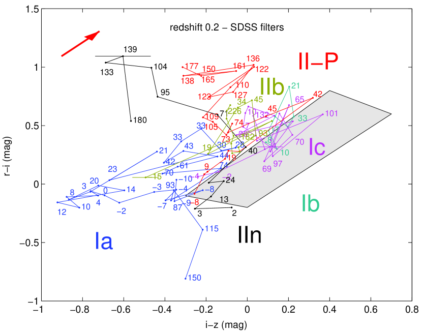
Figure 9: $r-i$ vs. $i-z$ for SNe of all types at $z=0.2$. The gray polygon includes the colors of almost all stars, cataclysmic variables, Cepheids, asteroids, and quasars from Krisciunas et al. (1998).

SNe are generally discovered by their variability. However, the tools developed in this paper may enable one to detect SNe by their colors alone. Indeed, such methods have recently been discussed for the detection of another kind of transient phenomenon — gamma-ray burst afterglows (Rhoads 2001). Multi-color wide-field surveys (e.g., Becker et al. 2001; Jannuzi et al. 2001; SDSS — York et al. 2000) that are either planned or already underway may be used to discover large numbers of SNe using similar methods. To illustrate this point, we plot in Figure 9 the locations of SNe of all types at $z=0.2$, together with a polygon within which fall the vast majority of stars, asteroids, cataclysmic variables, Cepheids, and quasars, as discussed by Krisciunas, Margon, & Szkody (1998). Except for late-time SNe Ic, all SNe have lower $i-z$ values and higher $r-i$ values than these objects. Similar results are obtained for the SN population at $z=$ 0–0.3, the redshifts of SNe probed by the SDSS. This demonstrates the feasibility of color selection of SNe, a method which may emerge as an invaluable resource when applied to upcoming, large data sets.

An exciting application of the methods presented in this paper would be the study of SNe discovered in the SDSS southern strip. During the months of September to November, when the primary target of the SDSS, the north Galactic pole, is not visible, the SDSS telescope observes parts of the sky near the south Galactic pole. The so called “south equatorial strip” is a patch of sky that will be imaged repeatedly during the 5-year planned operations of the survey. According to the SDSS website (http://www.sdss.org/documents/5yearbaseline.pdf), this 270 square degree area will be imaged $\sim 19$ times during the 5-year period, or about 4 times each fall, on average. Assuming that this sampling enables the discovery of all SNe that occur during the $\sim 3$ months this strip is imaged each year, for five years, the total surveyed area is $270\times 3\times 5$ deg²-months, or 337.5 deg²-years. Pain et al. (1996) have measured a SN Ia rate of 34 per year per square degree in the magnitude range $21.3\leq R\leq 22.3$, and the limiting magnitude of the SDSS images in this band is given as $r=22.5$ mag. We would then expect some 2300 SNe Ia each year or a total of over 11,000 SNe Ia in this strip. The numbers of SNe of all types (not just Ia) will undoubtedly be even larger. Miknaitis et al. (2001b) report that a systematic search for SNe in these data is underway, and the first SNe have already been reported (Miknaitis et al. 2001a; Rest, Miceli, & Covarrubias 2001; Miknaitis & Krisciunas 2001).

This huge expected dataset, which may contain an order of magnitude more events than all previously known SNe, all with five-band photometry and possibly some variability information, offers an unprecedented resource for SN studies. As an example, SN rates, based on thousands of events, can be computed as a function of SN type, host-galaxy morphology, and redshift. However, it is clear that obtaining spectra for thousands of faint SNe each fall is not feasible. Photometric classification could therefore be a valuable option. The SDSS supplies five-band information, along with ready-made tools for the derivation of photometric redshifts for all host galaxies, and spectral identification for part of the brighter ones. This makes our approach of using the SN photometry for classification, assuming that the redshift is known, even more appropriate. Since no followup is required, such an analysis need not be done in real time — in principle, it may even be carried out long after the project is complete, and all the data are publicly available.

In summary, we have presented a method for the classification of SNe, using multi-color broadband photometry. We have shown that the type of a SN may be uniquely determined in some cases. Even when this is not the case, constraints on the type may still be drawn. In particular, SNe Ia may be distinguished from core-collapse SNe during long periods in their evolution, for most of the redshifts and filter combinations studied. Finally, we have demonstrated the application of our method to a recently discovered SN from the SDSS, and we have shown how this technique may become a valuable tool for the analysis of the large SN samples expected to emerge from this and other programs that are already active or will begin soon. This work proves that spectroscopic followup is not always a prerequisite for SNe to be a valuable scientific resource, and lays the foundations for the exploitation of large SN samples for which such followup may not be possible.

Figure 1: Comparison between the synthetic colors (open circles, error bars calculated as explained in $\S~{}3.1$) of SNe Ia, and $UBV$ photometry (bold line) from Leibundgut (1988). The marked ages (here and in the following figures) are in days relative to $B$-band maximum. For clarity, we have sometimes omitted the age labels of data points with similar ages and colors. Many of the early-time (up to 2 weeks past maximum brightness) synthetic colors were derived from spectra of SN 1994D, which was somewhat bluer at those epochs than average SNe Ia; thus, from this plot we can estimate the expected width of color-color paths for normal SNe Ia to be $\sim 0.2$–0.3 mag.

Figure 2: Comparison of the synthetic colors (open circles, error bars calculated as above) for SNe II-P, with $UBV$ photometry of SN 1999em from Leonard et al. (2002a) for days $-1$ to 73 relative to $B$-band peak (bold line). Note that the three discordant points toward the lower-right corner are derived from spectra of SN 2001X (see $\S~{}3.1$ for discussion).

Figure 3: $U-B$ vs. $B-V$ (top), $B-V$ vs. $V-R$ (middle), and $V-R$ vs. $R-I$ (bottom) for SNe of all types at $z=0$. In this and all subsequent figures, the time evolution of each SN type is illustrated by linearly connecting, in temporal order, the locations occupied by such events. Note that we depict both branches of late-time evolution of type II-P SNe; see $\S~{}3.1$. The arrow shows the reddening effect of $A_{V}=1$ mag (in restframe $V$) extinction by dust in the host galaxy.

Figure 4: $V-R$ vs. $R-I$ for SNe of all types at $z=0.1$ (top) and $z=0.5$ (middle). At bottom, $r-i$ vs. $i-z$ for SNe of all types at $z=0.75$.

Figure 5: $I-J$ vs. $J-H$ for SNe of all types at $z=1$ (top), and $J-H$ vs. $H-K$ for SNe of all types at $z=1.5$ (bottom).

Figure 6: $U-B$ vs. $B-V$ (top) and $V-R$ vs. $R-I$ (middle) for normal (blue), SN 1991bg-like (black), SN 1991T-like (magenta), and SN 2000cx-like (green) SNe Ia at $z=0$. Bottom: same as top panel, but including core-collapse SNe of all types (red).

Figure 7: $r-i$ vs. $i-z$ for SNe Ia (black solid lines) and SNe Ic (grey dashed lines, italic age labels) at $z=0.6$.

Figure 8: $g-r$ vs. $r-i$ for SNe of all types at $z=0.0311$. The observed colors of SN 2001fg are indicated by the filled black circle. The colors suggest a SN Ia about 1 month past maximum brightness, as confirmed by spectra of this event.

Table 1: SN Spectral Database

Type	SNe	Epochs	Redshift	References
Ia	1994D	22	0.0015	1,9
	1987L	2	0.0074	1
	1995D	4	0.0066	9
	1999dk	5	0.0150	9
	1999ee	12	0.0114	10
Ib	1984L	12	0.0051	1,9
	1991ar	1	0.0152	2
	1998dt	2	0.0150	2
	1999di	1	0.0164	2
	1999dn	3	0.0093	2
Ic	1994I	14	0.0015	1,3
	1990U	8	0.0079	2
	1990B	4	0.0075	2
II-P	1999em	27	0.0024	4
	1992H	13	0.0060	1,9
	2001X	12	0.0049	6,9
IIn	1998S	13	0.0030	5,7
	1994Y	1	0.0080	1
	1994ak	1	0.0085	1
IIb	1993J	12	0	1
	1996cb	3	0.0024	8
Total		172

Table 2: Peculiar Type Ia SNe

Type	SNe	Epochs	Redshift	References
1991T-like	1991T	12	0.0058	1,5
	1998es	7	0.0106	5
1991bg-like	1991bg	5	0.0035	2,5
	1998bp	2	0.0104	5
	1998de	3	0.0166	5
	1999da	4	0.0127	5
2000cx-like	2000cx	23	0.0079	3,4
Total		56

References

- (1) Aldering, G., Supernova Cosmology Project Collaboration, & Nearby Supernova Factory Collaboration. 2001, BAAS, 199.67.01
- (2) Arnett, W. D., Bahcall, J. N., Kirshner, R. P., & Woosley, S. E. 1989, ARAA, 27, 629
- (3) Barbon, R., Ciatti, F., & Rosino, L. 1979, A&A, 72, 287
- (4) Becker, A., et al. 2001, BAAS, 199.1101.14; see also http://dls.bell-labs.com/team.html
- (5) Bessell, M. S., & Brett, J. M. 1988, PASP, 100, 1134
- (6) Brighenti, F., & Mathews, W. G. 1998, ApJ, 515, 542
- (7) Brighenti, F., & Mathews, W. G. 2001, ApJ, 553, 103
- (8) Brunner, R. J., Djorgovski, S. G., & Szalay, A. S. 2001, eds., Virtual Observatories of the Future (San Francisco: ASP, Conf. Ser. Vol. 225)
- (9) Cappellaro, E., et al. 1997, A&A, 322, 431
- (10) Cardelli, J. A., Clayton, G. C., & Mathis, J. S. 1989, ApJ, 345, 245
- (11) Clocchiatti, A., et al. 2000, ApJ, 529, 661
- (12) Coil, A. L., et al. 2000, ApJ, 544, L111
- (13) Cousins, A. W. J. 1976; see Moro & Munari 2000 for details
- (14) Dahlén, T., & Fransson, C. 1999, A&A, 350, 349
- (15) Dahlén, T., & Goobar, A. 2002, PASP, 114, 284 (DG2002)
- (16) Dimai, A. 2001, IAU Circ. 7719
- (17) Doggett, J. B., & Branch, D. 1985, AJ, 90, 2303
- (18) Fassia, A., et al. 2001, MNRAS, 325, 907
- (19) Filippenko, A. V. 1982, PASP, 94, 715
- (20) Filippenko, A. V. 1988, AJ, 96, 1941
- (21) Filippenko, A. V. 1997, ARA&A, 35, 309
- (22) Filippenko, A. V. 2001, PASP, 113, 1441
- (23) Filippenko, A. V., Barth, A. J., Bower, G. C., Ho, L. C., Stringfellow, G. C., Goodrich, R. W., & Porter, A. C. 1995a, AJ, 110, 2261 [Erratum: 112, 806 (1996)]
- (24) Filippenko, A. V., & Chornock, R. 2001, IAU Circ. 7754
- (25) Filippenko, A. V., Li, W. D., Treffers, R. R., & Modjaz, M. 2001, in Small-Telescope Astronomy on Global Scales, ed. W. P. Chen, C. Lemme, & B. Paczyński (San Francisco: ASP, Conf. Ser. 246), 121
- (26) Filippenko, A. V., Matheson, T., & Ho, L. C. 1993, ApJ, 415, L103
- (27) Filippenko, A. V., et al. 1992a, ApJ, 384, L15
- (28) Filippenko, A. V., et al. 1992b, AJ, 104, 1543
- (29) Filippenko, A. V., et al. 1995b, ApJ, 450, L11
- (30) Fukugita, M., Ichikawa, T., Gunn, J. E., Doi, M., Shimasaku, K., & Schneider, D. P. 1996, AJ, 111, 1748
- (31) Galama, T. J., et al. 1998, Nature, 395, 670
- (32) Gal-Yam, A., & Maoz, D. 1999, in “Cosmic Explosions,” ed. S. S. Holt & W. W. Zhang (New York: AIP), p. 107
- (33) Gal-Yam, A., & Maoz, D. 2000, IAU Circ. 7405
- (34) Gal-Yam, A., & Maoz, D. 2002, in preparation
- (35) Gal-Yam, A., Maoz, D., & Sharon, K. 2002, MNRAS, in press, astro-ph/0109089
- (36) Gal-Yam, A., & Shemmer, O. 2001, IAU Circ. 7602; see http://wise-obs.tau.ac.il/$∼$avishay/local.html
- (37) Germany, L. M., Reiss, D. J., Sadler, E. M., Schmidt, B. P., & Stubbs, C. W. 2000, ApJ, 533, 320
- (38) Goobar, A., & Perlmutter, S. 1995, ApJ, 450, 14
- (39) Hamuy, M., & Pinto, P. A. 2002, ApJL, 566, L63
- (40) Hamuy, M., et al. 2001, ApJ, 558, 615
- (41) Hamuy, M., et al. 2002, AJ, in press, astro-ph/0203491
- (42) Hardin, D., et al. 2000, IAU Circ. 7406
- (43) Höflich, P., Straniero, O., Limongi, M., Dominguez, I., & Chieffi, A. 2001, in Rev. Mexicana Astron. Astrofis. Ser. Conf. 10, The Seventh Texas-Mexico Conference on Astrophysics: Flows, Blows, and Glows, ed. W. Lee & S. Torres-Peimbert (Mexico, DF: Inst. Astron., UNAM), 157
- (44) Iwamoto, K., et al. 2000, ApJ, 534, 660
- (45) Jannuzi, B., et al. 2001; see http://www.noao.edu/noao/noaodeep
- (46) Johnson, H. L. 1965; see Moro & Munari 2000 for details
- (47) Jorgensen, H. E., Lipunov, V. M., Panchenko, I. E., Postnov, K. A., & Prokhorov, M. E. 1997, ApJ, 486, 110
- (48) Kirshner, R. P., & Kwan, J. 1974, ApJ, 193, 27
- (49) Krisciunas, K., Margon, B., & Szkody, P. 1998, PASP, 110, 1342
- (50) Leibundgut, B. 1988, Ph.D. Thesis, University of Basel
- (51) Leonard, D. C., Filippenko, A. V., Barth, A. J., & Matheson, T. 2000, ApJ, 536, 239
- (52) Leonard, D. C., et al. 2002a, PASP, 114, 35
- (53) Leonard, D. C., et al. 2002b, AJ, submitted
- (54) Li, W., Filippenko, A. V., Treffers, R. R., Riess, A. G., Hu, J., & Qiu, Y. 2001a, ApJ, 546, 734
- (55) Li, W., et al. 1996, IAU Circ. 6379
- (56) Li, W., et al. 2001b, PASP, 113, 1178
- (57) Loewenstein, M. 2000, ApJ, 532, 17
- (58) Madau, P., Della Valle, M., & Panagia, N. 1998, MNRAS, 297, L17
- (59) Matheson, T., Filippenko, A. V., Li, W., Leonard, D. C., & Shields, J. C. 2001, AJ, 121, 1648
- (60) Matteucci, F., & Greggio, L. 1986, A&A, 154, 279
- (61) Miknaitis, G., & Krisciunas, K. 2001, IAU Circ. 7778
- (62) Miknaitis, G., Miceli, A., Stubbs, C., Covarrubias, R., & Lawton, B. 2001a, IAU Circ. 7731
- (63) Miknaitis, G., Rest, A., Stubbs, C., Stoughton, C., & SDSS Collaboration. 2001b, BAAS, 199.84.04
- (64) Miller, D. L., & Branch, D. 1990, AJ, 100, 530
- (65) Minkowski, R. 1941, PASP, 53, 224
- (66) Moro, D., & Munari, U. 2000, A&AS, 147, 361
- (67) Pain, R., et al. 1996, ApJ, 473, 356
- (68) Parodi, B. R., Saha, A., Sandage, A., & Tammann, G. A. 2000, ApJ, 540, 634
- (69) Patat, F., et al. 2001, ApJ, 555, 900
- (70) Perlmutter, S., et al. 1997, ApJ, 483, 565
- (71) Perlmutter, S., et al. 1999, ApJ, 517, 565
- (72) Perlmutter, S., & SNAP Collaboration. 2000, BAAS, 197.61.01
- (73) Phillips, M. M., Lira, P., Suntzeff, N. B., Schommer, R. A., Hamuy, M., & Maza, J. 1999, AJ, 118, 1766
- (74) Qiu, Y., & Hu, J. Y. 2001, IAU Circ. 7753
- (75) Qiu, Y., Li, W., Qiao, Q., & Hu, J. 1999, AJ, 117, 736
- (76) Reiss, D., Germany, L. M., Schmidt, B. P., & Stubbs, C. W. 1998, AJ, 115, 26
- (77) Rest, A., Miceli, A., & Covarrubias, R. 2001, IAU Circ. 7740
- (78) Rhoads, J. E. 2001, ApJ, 557, 943
- (79) Richards, G. T., et al. 2001, AJ, 122, 1151
- (80) Richmond, M. W. et al. 1995, AJ, 109, 2121.
- (81) Riess, A. G., et al. 1998, AJ, 116, 1009
- (82) Riess, A. G., et al. 1999, AJ, 117, 707
- (83) Riess, A. G., et al. 2001, ApJ, 560, 49
- (84) Ruiz-Lapuente, P., & Canal, R. 1998, ApJ, 497, L57
- (85) Sadat, R., Blanchard, A., Guiderdoni, B., & Silk, J. 1998, A&A, 331, L69
- (86) Schaefer, B. E. 2000, IAU Circ. 7387
- (87) Schlegel, D. J., Finkbeiner, D. P., & Davis, M. 1998, ApJ, 500, 525
- (88) Schlegel, E. M. 1990, MNRAS, 244, 269
- (89) Schmidt, B. P., Kirshner, R. P., & Eastman, R. G. 1992, ApJ, 395, 366
- (90) Schmidt, B. P., et al. 1994, ApJ, 432, 42
- (91) Schmidt, B. P., et al. 1998, ApJ, 507, 46
- (92) Stoughton, C., et al. 2002, AJ, 123, 485
- (93) Sullivan, M., Ellis, R., Nugent, P., Smail, I., & Madau, P. 2000, MNRAS, 319, 549
- (94) Treffers, R. R., Peng, C. Y., Filippenko, A. V., & Richmond, M. W. 1997, IAU Circ. 6627
- (95) Tripp, R. 1998, A&A, 331, 815
- (96) Turatto, M., et al. 2000, ApJ, 534, 57
- (97) Vanden Berk, D. E., et al. 2001, BAAS, 199.84.05
- (98) Van Dyk, S. D., Peng, C. Y., King, J. Y., Filippenko, A. V., Treffers, R. R., Li, W., & Richmond, M. W. 2000, PASP, 112, 1532
- (99) Weymann, R. J., Storrie-Lombardi, L. J., Sawicki, M., & Brunner, R. 1999, eds., Photometric Redshifts and High-Redshift Galaxies (San Francisco: ASP)
- (100) York, D. G., et al. 2000, AJ, 120, 1579
- (101) Yungelson, L., & Livio, M. 2000, ApJ, 528, 108