Measuring Feedback Using the Intergalactic Medium State and Evolution Inferred from the Soft X-ray Background

Abstract

We explore the intergalactic medium (IGM) as a potential source of the unresolved soft X-ray background (XRB) and the feasibility to extract the IGM state and evolution from XRB observations. We build two analytical models, the continuum field model and the halo model, to calculate the IGM XRB mean flux, angular auto correlation and cross correlation with galaxies. Our results suggest that the IGM may contribute a significant fraction to the unresolved soft XRB flux and correlations. We calibrated non-Gaussian errors estimated against our $512^{3}$ moving mesh hydro simulation and estimate that the ROSAT all sky survey plus Sloan galaxy photometric redshift survey would allow a $\sim 10\%$ accuracy in the IGM XRB-galaxy cross correlation power spectrum measurement for $800<l<5000$ and a $\sim 20\%$ accuracy in the redshift resolved X-ray emissivity-galaxy cross correlation power spectrum measurement for $z\lesssim 0.5$. At small scales, non-gravitational heating, e.g. feedback, dominates over gravity and leaves unique signatures in the IGM XRB, which allows a comparable accuracy in the measurement of the amount of non-gravitational heating and the length scales where non-gravitational energy balances gravity.

1 Introduction

A large fraction of the intergalactic medium (IGM) is hot. The cosmic virial theorem predicts that the mean IGM temperature $>0.2$ keV (Pen, 1999). It emits X-ray through thermal bremsstrahlung and contributes to the soft (0.5-2 keV) X-ray background (XRB). About $80$-$90\%$ of the soft XRB has been resolved into point objects such as AGNs (Hasinger et al., 1993). Various sources such as nearby low luminosity AGNs (Halderson et al., 2001), unresolved galactic stars (Kuntz & Snowden, 2001), galactic gas, X-ray sources in external galaxies and the IGM (Pen, 1999; Wu & Xue, 2001; Croft et al., 2001) may contribute a significant fraction to the remaining $10$-$20\%$. To distinguish those possible components, one can combine the XRB mean flux, auto correlation (Soltan & Hasinger, 1994; Sliwa, Soltan & Freyberg, 2001) and cross correlation with galaxies (Almaini et al., 1997; Refregier, Helfand & Mcmahon, 1997). In §2, we will build analytical models to estimate the IGM contribution to the XRB flux and correlations.

In pure gravitational clustering where the only source of thermal energy is shock heating from collapse, simulations show that the gas correlation function $\xi_{\rm gas}$ follows the dark matter correlation function down to scales where the gas over-density correlation $\xi_{\rm gas}\sim 10^{3}$ (Pen, 1999). Non-gravitational heating (feedback) can rearrange the gas distribution on small scales. By searching for the scale where feedback dominates over gravity, one can robustly measure the strength and history of non-gravitational heating. The IGM XRB is sensitive to small scale gas structures due to the X-ray emissivity dependence on density squared. This makes the IGM XRB a potentially powerful probe for studying feedback from galaxies on the IGM. From the estimation of the IGM XRB flux, Pen (1999); Wu, Fabian & Nulsen (2001); Voit & Bryan (2001) suggested that, if only gravitational heating exists, the soft X-ray emission that the IGM produces would exceed the observational limit. To suppress the IGM clumping and reduce the X-ray emission, a significant amount of non-gravitational injection energy $\sim 1$ keV/nucleon is required. Croft et al. (2001); Dave et al. (2001); Phillips et al. (2001) argued from simulations that such energy injection is not necessary. In their simulations, a large fraction of baryons (about $70\%$) are too cold to contribute significantly to the XRB. Despite the stability problem of cool gas, these findings may indicate a degeneracy between non-gravitational heating and the fraction of IGM contributing to the XRB. The IGM XRB auto correlation function (ACF) and cross correlation function (CCF) with galaxies have different dependences on the IGM thermal state and are capable of breaking this degeneracy. Furthermore, with galaxy photometric redshift data, the redshift resolved IGM X-ray emissivity-galaxy cross correlation and emissivity auto correlation can be extracted. This tells the evolution of the IGM state. In §3, we will forecast the sensitivity of ROSAT all sky survey (Voges et al., 1999) and SDSS and test the feasibility to constrain the IGM thermal history from correlations. This estimation depends on the XRB non-Gaussianity since it affects the error analysis. We analyze our $512^{3}$ moving mesh hydro simulation to quantify this effect.

2 Analytical models for the IGM XRB

The X-ray emissivity in the band $E_{1}\leq h\nu\leq E_{2}$ is given by: $I_{X}\simeq 2.4\times 10^{-27}c_{Z}T^{1/2}[\exp(-E_{1}/T)-\exp(-E_{2}/T)]n_{e}^{2}\equiv\Lambda_{E_{1}}^{E_{2}}(T)n_{e}^{2}\ {\rm erg\ cm^{-3}\ s^{-1}}$ (Tucker, 1975). $\Lambda_{E_{1}}^{E_{2}}(T)$ is the cooling coefficient in the energy band $E_{1}$-$E_{2}$. A mean gaunt factor $1.2$ is adopted. $c_{Z}\sim Z/Z_{\sun}(4{\rm keV}/T)+1$ is a fitting formula to result of metal cooling from Raymond, Cox & Smith (1976). We will use $Z=\frac{1}{4}Z_{\sun}$ as the lower plausible limit on the IGM inferred from clusters of galaxies. We choose a flat $\Lambda$CDM cosmology with $\Omega_{0}=0.37$, $\Omega_{\Lambda}=0.63$, $\Omega_{B}=0.04$, $\sigma_{8}=0.9$, $h=0.7$ and $n=1$ to calculate the soft XRB statistics. Hereafter, we always consider the comoving emissivity $I_{X}^{C}=I_{X}/(1+z)^{3}$.

The IGM XRB flux $F_{X}(\hat{\theta})=\int I^{C}_{X}(\chi\hat{\theta})/[4\pi(1+z)^{2}]d\chi$. $\chi$ is the comoving distance. The mean XRB flux $\bar{F}_{X}=\int\bar{I}^{C}_{X}/[4\pi(1+z)^{2}]d\chi$. The galaxy surface density $\Sigma(\hat{\theta})=\int\frac{dn}{dz}[1+\delta_{G}(\chi\hat{\theta})]dz.$ $\frac{dn}{dz}$ is the galaxy redshift distribution and $\delta_{G}$ is the galaxy number over-density. The mean surface density $\bar{\Sigma}=\int\frac{dn}{dz}dz$. We define the dimensionless fluctuations $\Delta_{F}\equiv F/\bar{F}-1$ and $\Delta_{\Sigma}\equiv\Sigma/\bar{\Sigma}-1$. The IGM XRB ACF and CCF with galaxies are defined by $w_{X}(\theta)\equiv\langle\Delta_{F}(\hat{\theta}_{1})\Delta_{F}(\hat{\theta}_{2})\rangle$ and $w_{XG}(\theta)\equiv\langle\Delta_{F}(\hat{\theta}_{1})\Delta_{\Sigma}(\hat{\theta}_{2})\rangle$, respectively. Here, $\hat{\theta}_{1}\cdot\hat{\theta}_{2}=\cos\theta$. $C^{X}(l)$ and $C^{XG}(l)$ are the corresponding angular power spectra, respectively.

These 2D correlations are determined by the corresponding 3D correlations such as the emissivity ACF $\xi_{X}(r)\equiv\langle\delta_{X}({\bf x})\delta_{X}({\bf x+r})\rangle$ and emissivity-galaxy CCF $\xi_{XG}(r)=\langle\delta_{X}({\bf x})\delta_{G}({\bf x+r})\rangle$ or their corresponding power spectra $P_{X}(k,z)$ and $P_{XG}(k,z)$. $\delta_{X}\equiv I^{C}_{X}/\bar{I}^{C}_{X}-1$. At small angular scales we use the Limber’s equation to obtain

$$C^{X}(l)=\frac{1}{\bar{F}_{X}^{2}}\int_{0}^{\chi_{\rm re}}P_{X}(\frac{l}{\chi},z)\frac{[\bar{I}_{X}^{C}(z)]^{2}}{[4\pi(1+z)^{2}]^{2}\chi^{2}}d\chi,$$ (1)

$$C^{XG}(l,z_{1},z_{2})=\frac{1}{\bar{F}_{X}\bar{\Sigma}}\int_{z_{1}}^{z_{2}}P_{XG}(\frac{l}{\chi},z)\frac{\bar{I}_{X}^{C}(z)}{4\pi(1+z)^{2}\chi^{2}}\frac{dn}{dz}dz.$$ (2)

Here, $\chi_{\rm re}$ is the comoving distance to the reionization epoch. $[z_{1},z_{2}]$ is the redshift range of the galaxy survey adopted.

For these statistics, we can treat the IGM either as a continuum field with a density and temperature distribution or as discrete halos. From these two viewpoints, we build two analytical models: the continuum field model (§2.1) and the halo model (§2.2).

Figure 1: The IGM cumulative contribution to the XRB. Contribution with different $k_{\rm gas}$ looks similar.

2.1 The continuum field model

For the $[0.5,2]$ keV X-ray band, we can approximate the gas temperature $T\simeq 1$ keV due to the following arguments. (1) when $T\ll 1$ keV, $\Lambda_{E_{1}}^{E_{2}}(T)$ decreases exponentially and we would expect that too cold gas does not contribute significantly to the soft XRB. (2) When $T\gg 1$ keV, $\Lambda_{E_{1}}^{E_{2}}(T)$ drops as $T^{-1/2}$. Furthermore, gas with $T\gg 1$ keV is rare. So the contribution from gas with $T\gg 1$ keV to the soft XRB is small. (3) $\Lambda_{E_{1}}^{E_{2}}(T)$ peaks at $T\sim 1$ keV. The density weighted temperature is $\sim 0.4$ keV (Zhang & Pen, 2001) and the density square weighted (roughly emissivity weighted) temperature $\sim 1$ keV. So, we expect most contributions to the soft XRB to be from gas with $T\sim 1$ keV. Around this temperature, the emissivity has only a weak temperature dependence. So, we approximate $T=1$ keV and define a X-ray weighted gas fraction $f^{X}_{\rm gas}\equiv\sqrt{I_{X}/[\Lambda_{E_{1}}^{E_{2}}(1\ {\rm keV})n_{e}^{2}]}$. From the above argument we expect $f^{X}_{\rm gas}\simeq 1$, but throughout this letter, we treat $f^{X}_{\rm gas}$ as a free parameter to be determined by observations. At large scales, gas generally follows dark matter. At smaller scales, the gas density fluctuation is suppressed by the gas pressure. This effect can be modeled through a window function $W_{g}(r)$ such that the gas over-density is a convolution of the dark matter density and $W_{g}(r)$. The FWHM of $W_{g}(r)$ is the scale where non-gravitational processes such as feedback begins to dominate over gravity. In Fourier space, the Fourier component of the gas over-density $\delta_{\rm gas}(k)=\delta(k)W_{\rm gas}(k)$ where $\delta(k)$ is the Fourier component of the dark matter over-density. A Gaussian window function $W_{\rm gas}(k)=\exp(-k^{2}/k_{\rm gas}^{2})$ is choose from the literature (Gnedin & Hui, 1998). With the correlation between gas and dark matter, one can calculate the XRB statistics using the knowledge of dark matter density field.

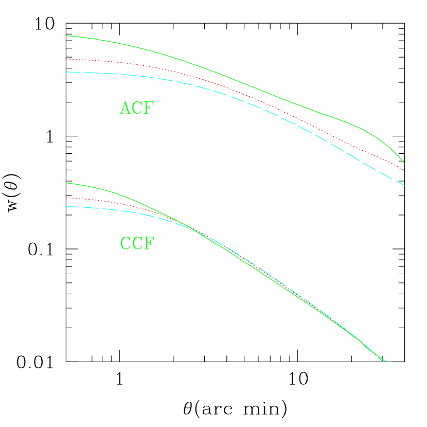
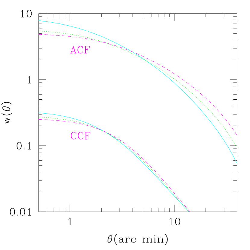
Figure 2: IGM XRB angular ACF $w_{X}(\theta)$ and CCF $w_{XG}(\theta)$ calculated from the continuum field model (left panel) and the halo model (right panel). The solid, dot, dash lines correspond to $k_{\rm gas}=8,4,3h/$Mpc ( corresponds to non-gravitational heating energy per nucleon $E_{\rm NG}\sim 0.3,0.6,0.9$ keV) in the left panel and $r_{c}(M_{8},z=0)=0.5,0.75,1.0h^{-1}$ Mpc ($E_{\rm NG}\sim 0.5,0.6,0.8$ keV) in the right panel. $k_{\rm gas}$ and $r_{c}$ are the scales below which feedback dominates over gravity. The slopes of $w(\theta)$ predicted by the halo model are steeper than the continuum field results. This difference is likely due to the weak correlation between density and temperature, which is omitted in the continuum field model.

We apply the extension of the hierarchical model (Fry, 1984) in the highly non-linear regime: the hyper-extended perturbation theory (HEPT) (Scoccimarro & Frieman, 1999) to calculate $P_{X}$ and $P_{XG}$.

$$P_{X}(k,z)\simeq\frac{1}{\sigma_{\rm gas}^{4}(2\pi)^{6}}\int B_{4}({\bf k_{1}},{\bf k_{2}},{\bf k_{3}},{\bf k_{4}};z)W_{1}W_{2}W_{3}W_{4}d^{3}k_{2}d^{3}k_{4}$$ (3)

$$P_{XG}(k,z)\simeq\frac{1}{\sigma_{\rm gas}^{2}(2\pi)^{3}}\int bB_{3}({\bf k}_{1},{\bf k}_{2},{\bf k};z)W_{1}W_{2}d^{3}k_{1}.$$ (4)

Here, $W_{i}=W_{\rm gas}(k_{i})$, ${\bf k_{1}}+{\bf k_{2}}=-{\bf k_{3}}-{\bf k_{4}}={\bf k}$. The gas clumping factor $\sigma_{\rm gas}^{2}=\int P_{\rm gas}(k)k^{2}dk/(2\pi^{2})$ with $P_{\rm gas}(k)$ as the gas density power spectrum. The bispectrum $B_{3}\propto P^{2}(k)$ and polyspectrum, the dominant term in the expression of $P_{X}(k,z)$, $B_{4}\propto P^{3}(k)$ terms are calculated from HEPT. Here, $P(k)$ is the dark matter density power spectrum. See Zhang & Pen (2001) for more detailed explanation. We consider a flux limited galaxy survey SDSS, take the SDSS galaxy distribution as $\frac{dn}{dz}=\frac{3z^{2}}{2(z_{m}/1.412)^{3}}\exp[-(1.412z/z_{m})^{3/2}]$ (Baugh & Efstathiou, 1993) and adopt $z_{m}=0.43$ as the median redshift of Sloan galaxy photometric redshift distribution (Dodelson et al., 2001). We assume that $k_{\rm gas}$ does not change with redshift and a constant bias model $\delta_{G}=b\delta$ for galaxies.

2.2 The halo model

The gas profile in a halo and halo mass-temperature relation determines the X-ray luminosity. The halo mass function and halo-halo correlation enable us to calculate their collective effects to the XRB. Similar methods have been applied to the dark matter correlation (Ma & Fry, 2000) and the Sunyaev-Zel’dovich effect (Komatsu & Kitayama, 1999).

We adopt the electron number density profile $n_{e}=n_{0}\left[1+(\frac{r^{2}}{r_{c}^{2}})\right]^{-1}$. The gas core radius $r_{c}$ is analogous to $k_{\rm gas}$ and corresponds to the scale below which feedback significantly changes gravitational clustering. We assume that gas accounts for $\Omega_{B}/\Omega_{0}=11\%$ of the halo mass. The gas temperature is determined by the virial theorem through the relation $\frac{M}{M_{8}}=\left[\frac{T/{\rm keV}}{4.9\Omega_{0}^{2/3}\Omega(z)^{0.283}(1+z)}\right]^{3/2}$ (Pen, 1998). $M_{8}$ is the mean mass contained in a $8h^{-1}{\rm Mpc}$ sphere today. The distribution of halo comoving number density $n$ as a function of halo mass $M$ and $z$ is given by (Press & Schechter, 1974): $\frac{dn}{dM}=(\frac{2}{\pi})^{1/2}\frac{\rho_{0}}{M^{2}}\frac{\delta_{c}}{\sigma}|\frac{d\rm{ln}\sigma}{d{\rm{ln}}M}|\exp(-\frac{\delta_{c}^{2}}{2\sigma^{2}})$. Here $\rho_{0}$ is the present mean matter density of the universe. $\sigma(M,z)$ is the linear theory rms density fluctuation in a sphere containing mass M at redshift $z$. $\delta_{c}$ is the linearly extrapolated over-density at which an object virializes. Its dependence on cosmology is weak and we will adopt the value $1.686$, which is the $\delta_{c}$ for a $\Omega_{0}=1.0$ CDM universe Eke, Cole & Frenk (1996). Mo & White (1996) related the halo-halo correlation $P_{c}(M_{1},M_{2})$ with the underlying dark matter correlation $P(k)$ by a linear bias: $P_{c}(k,M_{1},M_{2})=P(k)b(M_{1})b(M_{2})$. We adopt the NFW profile (Navarro et al., 1996) with a compact parameter $c=5$ to calculate the XRB-dark matter cross correlation.

In this model, the variance of the gas density $\sigma_{\rm gas}^{2}\propto\int_{M_{\rm low}}^{\infty}n_{0}^{2}r_{c}^{3}[\tan^{-1}(r_{\Delta}/r_{c})-\frac{r_{\Delta}/r_{c}}{1+(r_{\Delta}/r_{c})^{2}}]\frac{dn}{dM}dM$. $r_{\Delta}$ is the virial radius and we calculate it using the fitting formula of Eke, Cole & Frenk (1996). Defining $\delta_{X}({\bf k},M)$ and $\delta({\bf k},M)$ as the Fourier transform of $I^{C}_{X}({\bf r},M)/\bar{I}^{C}_{X}$ and $\delta({\bf r},M)\equiv\rho_{DM}({\bf r},M)/\bar{\rho}_{DM}$ of each halo, respectively, we obtain

$$P_{X}(k)=\frac{1}{\bar{I}_{X}^{2}}\left(\int_{M_{\rm low}}^{\infty}\delta_{X}^{2}(k)\frac{dn}{dM}dM+P(k)\left[\int_{M_{\rm low}}^{\infty}\delta_{X}(k)\frac{dn}{dM}dMb(M)\right]^{2}\right),$$ (5)

$$P_{X\delta}(k) = \frac{1}{\bar{I}_{X}}\left(\int_{M_{\rm low}}^{\infty}\delta_{X}(k)\delta(k)\frac{dn}{dM}dM+\right.$$

$$\left.P(k)\left[\int_{M_{\rm low}}^{\infty}\delta_{X}(k)\frac{dn}{dM}dMb(M)\right]\left[\int_{M_{\rm low}}^{\infty}\delta(k)\frac{dn}{dM}dMb(M)\right]\right).$$

The integrals in these equations depend strongly on the halo lower mass limit $M_{\rm low}$, which can not be arbitrarily chosen. A smaller $M_{\rm low}$ will produce a bigger gas clumping factor $\sigma^{2}_{\rm gas}$ since more gas contributes. It will also produce a smaller $P_{X}$ since gas in less massive halos is more diffuse and contributes a smaller fraction to the correlation than to the mean flux. This behavior contradicts the $P_{X}\propto\sigma^{2}_{\rm gas}$ behavior we should expect. Thus $M_{\rm low}$ must be determined independently. Here we adopt the model of Pen (1999). In this model, the energy injection from feedback such as supernovae winds expand the gas and produces a core (radius $r_{1}(M)$) with a constant entropy. Then $r_{1}(M)=r_{\Delta}(M)$ sets the value of $M_{\rm low}$. In this model, $r_{1}\simeq 0.5r_{c}\propto T^{-1}\propto M^{-2/3}$. We further assume $r_{c}(M_{8},z)=r_{c}(M_{8},z=0)/(1+z)$, which corresponds to a redshift independent $k_{\rm gas}$.

2.3 Predictions

Two models give consistent predictions for the XRB. More than $80\%$ of the contribution to the soft XRB flux is from the IGM at $z\leq 1$ (fig. 1). The mean X-ray flux $\bar{F}_{X}\simeq(\frac{\sigma_{g}^{2}}{30})10^{-12}\ {\rm erg}\ {\rm s}^{-1}\ {\rm cm}^{-2}\ {\rm deg}^{-2}$, which accounts for a significant, if not dominant, fraction of the unresolved XRB. The IGM XRB is homogeneous with a large amplitude (fig. 2) and is sufficient to explain the observed XRB correlations. The point-to-point XRB variance $W_{X}(0)\sim 10$ and $W_{XG}(0)\sim 0.3$. For $\theta>1^{{}^{\prime}}$, we find that $W_{XG}\propto\theta^{\alpha}$ ($\alpha\sim-1.1$). The shape and amplitude of these properties have different dependences on gas parameters. (1) For the shapes, the larger $k_{\rm gas}$ (corresponds to a smaller $r_{c}$ and a larger $\sigma_{\rm gas}^{2}$), the steeper the correlations. (2) For the amplitudes, $\bar{F}_{X}\propto(f^{X}_{\rm gas})^{2}\sigma_{\rm gas}^{2}$ while $P_{X}(k),P_{XG}(k),w_{X}(0),w_{XG}(0)\propto(f^{X}_{\rm gas})^{0}\sigma_{\rm gas}^{2}$. Combining correlation data and mean flux data, one can distinguish $f_{\rm gas}^{X}$ from $\sigma_{\rm gas}^{2}$. With redshift resolved $P_{X}(k,z)$ or $P_{XG}(k,z)$, as can be obtained from XRB observations and galaxy surveys, one can infer $\sigma_{\rm gas}^{2}(z)$ and then $k_{\rm gas}(z)$ and $r_{c}(z)$ from their relations with $\sigma_{\rm gas}^{2}(z)$. The interpretation of these quantities depends on processes changing the gas-dark matter correlation such as non-gravitational heating and possibly gravitational shock-heating. Current simulations have difficulties to resolve these small scales where these processes become dominant due to limited simulation mass and spatial resolution. Simulation results about the IGM XRB flux, hot gas fraction, etc. have not converged, so hereafter we focus on the estimation of the effect of feedback through our analytical models and use our hydro simulation to calibrate some XRB statistics. Feedback increases the gas temperature and thus $f_{\rm gas}^{X}$, the fraction of gas contributing to XRB. But it dilutes the gas and reduces $\sigma_{\rm gas}^{2}$, resulting in a larger $r_{c}$ or a smaller $k_{\rm gas}$. From Pen’s model, for a $\Lambda$CDM universe, we can estimate $E_{\rm NG}(z)$, the non-gravitational energy injection per nucleon in unit of keV, from the relation $\sigma_{\rm gas}^{2}\simeq 90\Omega_{0}[2\sqrt{E_{NG}}\exp(-E_{\rm NG})+\sqrt{\pi}{\rm erfc}(\sqrt{E_{\rm NG}})]/E_{\rm NG})$. $k_{\rm gas}(z)$ (or $r_{c}$) and $E_{\rm NG}(z)$ then tell us the scales at which feedback dominates over gravity and the feedback strength.

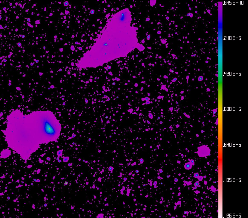
Figure 3: A XRB map in our $512^{3}$ MMH simulation(Zhang, Pen & Wang, 2002). The parameters we adopted in this simulation are $\Omega_{0}=0.37$, $\Omega_{\Lambda}=0.63$, $\Omega_{B}=0.05$, $h=0.7$, $\sigma_{8}=1.0$, the primordial power spectrum index $n=1$, box size $L=100h^{-1}$ Mpc and smallest grid spacing $40h^{-1}$ kpc. The XRB map integrates contributions up to $z=3$ and has a width of $1.32$ degree. The XRB flux is in units of ${\rm erg}\ {\rm s}^{-1}\ {\rm cm}^{-2}\ {\rm sr}^{-1}$.

Figure 4: The XRB-galaxy cross correlation non-Gaussian corrections $\eta(l)$ from sample variance errors measured from our $512^{3}$ MMH simulation. For Gaussian signals, $\eta(l)=0$. We make $40$ XRB maps and $40$ maps of the intergalactic gas surface density at the same fields of view to measure the XRB-galaxy cross correlation assuming that galaxy number density traces the gas distribution. We then measure the fluctuation of the cross correlation power spectra of these maps to obtain the XRB-galaxy cross correlation power spectrum non-Gaussianity $\eta(l)$. We find a strong non-Gaussian correction at scales $500<l<10^{4}$.

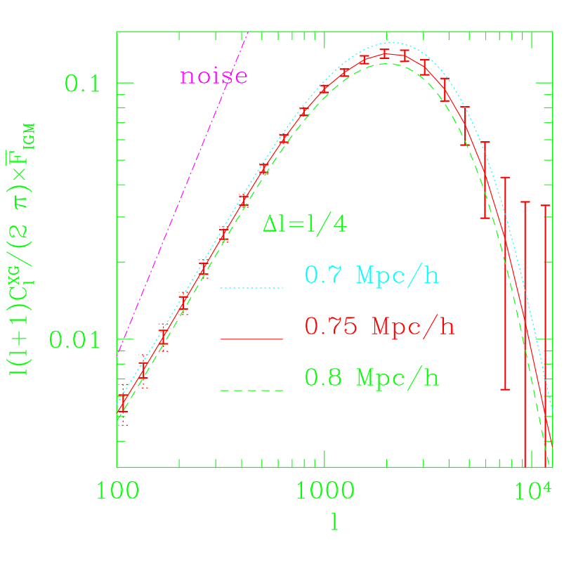
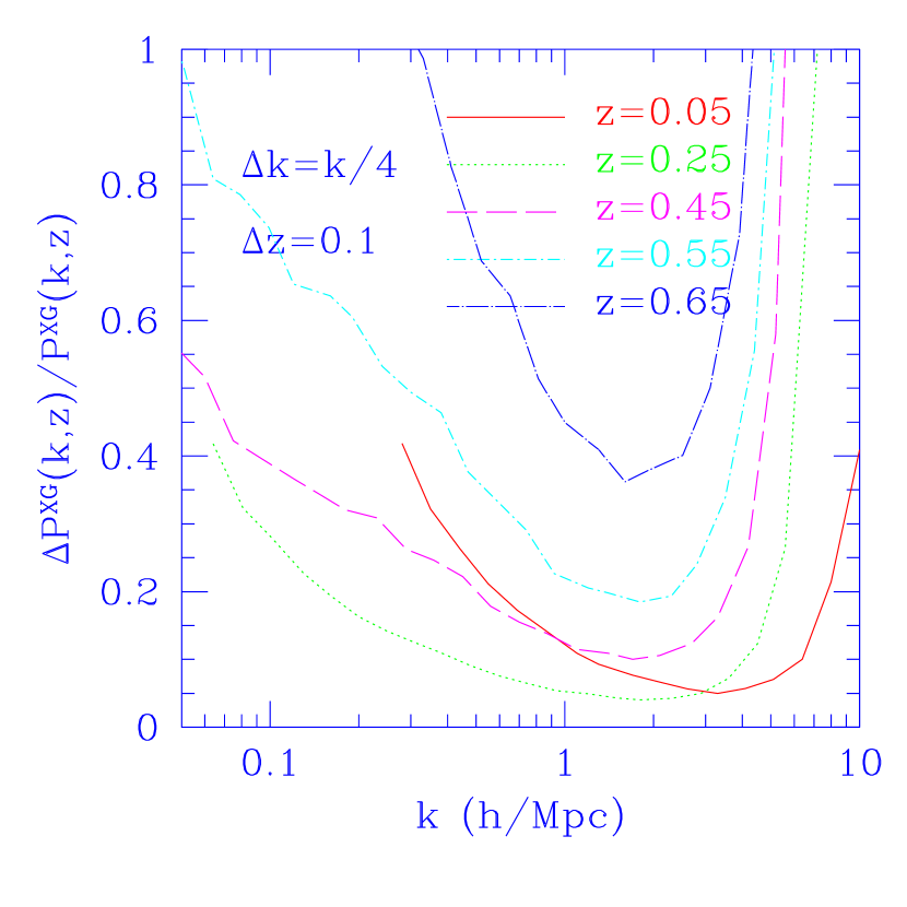
Figure 5: Statistical errors in the forecast ROSAT+SDSS measurement of $\frac{l(l+1)}{2\pi}C^{XG}(l)\bar{F}^{\rm IGM}_{X}$ (left panel) and extracted $P_{XG}(k,z)$ (right panel). In the left panel, error bars are for the central line with $r_{c}(M_{8},z=0)=0.75h^{-1}$ Mpc and we normalize its $\bar{F}^{\rm IGM}_{X}=1$. Solid error bars are Gaussian errors and the dot error bars are non-Gaussian errors. The effect of non-Gaussianity is dominant at large angular scales and is negligible at small angular scales where the dominant error is from noise. The redshift averaged gas parameter $r_{c}$ can be constrained with $\sim 10\%$ accuracy at $1\sigma$. The amount of feedback and the scale below which feedback dominates over gravity can be modeled with a comparable accuracy as $P_{XG}(k,z)$.

3 Extracting the IGM state and evolution

X-ray sources and differential extinction of our galaxy make the measurement of the IGM XRB flux and ACF difficult. But the measurement of IGM XRB-galaxy CCF is much more robust. The direct observable in the CCF measurement is $\langle F_{X}(\hat{\theta}_{1})\Sigma_{G}(\hat{\theta}_{2})\rangle$. We need to estimate the IGM contribution to the above property in order to infer $w_{XG}^{\rm IGM}(\theta)$. (1) Our calculation suggests that the IGM XRB is sufficient to explain the unresolved X-ray flux and the cross correlation with galaxies. (2) Distant AGNs and galactic X-ray sources have almost no correlation with nearby galaxies with $z\lesssim 1$. (3) The CCF between galaxies and X-ray sources in extragalactic galaxies or nearby low luminosity AGNs is of the same amplitude of galaxy surface density ACF, which is one order of magnitude lower than the IGM XRB-galaxy CCF. So, even if they contribute a comparable amount to the XRB flux as the IGM, their contribution to the cross correlation is negligible. (4) For a low matter density universe, the CCF caused by the weak lensing of low redshift large scale structures to unresolved high redshift AGNs accounts for at most $1/3$ of the correlation (Cooray, 1999). In principle, combining the XRB mean flux, auto correlation and cross correlation measurement, the IGM XRB cross correlation can be determined. We neglect possible systematic errors in such measurements and take the ROSAT all sky survey and SDSS as our targets to estimate the statistical error in the IGM XRB CCF measurement.

The ROSAT all sky survey (RASS) covers the whole sky ($f^{\rm RASS}_{\rm sky}\simeq 1$) in the $0.1$-$2.4$ soft X-ray band in $t=1.03\times 10^{7}$ s. At the energy bands below $0.5$ keV, the galactic emission and absorption are strong and at bands $>1$ keV, only a fraction of the sky can be used. So, we choose the band $0.5$-$1$ keV for our analysis. A factor of $4$ decrease in the photon count rate is expected due to the choice of this band instead of the whole RASS band. One full field view of RASS has a $\sim 1$ degree radius and only within the central $10$-$15$ arc-min radius is the resolution better than $3$ arc-min. Since we need high resolution to probe the IGM state, we will focus on these central regions. Since the separation of two successive scans is smaller than $10$ arc-min, these high resolution regions cover almost the whole sky. But the number of photons received in these regions is about $1/36$-$1/16$th of the total number of photons received. We adopt the conservative fraction $1/36$ for our following estimation. The SDSS covers $f^{\rm SDSS}_{\rm sky}\simeq 1/4$ fraction of the sky and will detect about $N_{G}=5\times 10^{7}$ galaxies. We estimate the error in the power spectrum $C_{l}$ measurement. The error in the IGM XRB-galaxy power spectrum is

$$\Delta C_{l}^{XG}=\sqrt{\frac{(\eta(l)+1)[C^{XG}_{l}]^{2}+(C^{X}_{l}+C_{N}^{X})\times(C^{G}_{l}+C_{N}^{G})}{(2l+1)\Delta lf^{\rm SDSS}_{\rm sky}}}.$$ (7)

$C^{G}$ is the power spectrum of the galaxy surface density. $C_{N}^{G}(l)=4\pi f^{\rm SDSS}_{\rm sky}/N_{G}$ is the Poisson noise of the galaxy number count. $C_{N}^{X}(l)=4\pi f^{\rm RASS}_{\rm sky}(\bar{F}_{N}/\bar{F}_{X})^{2}/N_{N}+4\pi f^{\rm RASS}_{\rm sky}/N_{X}$, where the first term is the Poisson noise of the RASS background and the second term is the Poisson noise of the IGM XRB signal. $N_{N}$ and $N_{X}$ are the total numbers of photons that the RASS received in the band $0.5$-$1$ keV from background noise and the IGM, respectively. We adopt $\bar{F}_{N}(0.1$-$2.4$ keV$)\simeq 5\times 10^{-12}{\rm erg}\ {\rm cm}^{-2}\ {\rm s}^{-1}{\rm deg}^{-2}$ (Fig. 3, Voges et al. (1999)). $\Delta l$ is the bin width and $f_{\rm sky}^{\rm SDSS}$ reflects the cosmic variance. The strong non-Gaussianity of the XRB affects its error analysis. One could in practice estimate $\eta(l)$, the non-Gaussianity of the XRB-galaxy cross correlation power spectrum (for Gaussian case, $\eta=0$) from our models. For simplicity, we will adopt the result from our $512^{3}$ moving mesh hydro (MMH) simulation (Zhang, Pen & Wang, 2002). The parameters we adopted in our $512^{3}$ simulation are $\Omega_{0}=0.37$, $\Omega_{\Lambda}=0.63$, $\Omega_{B}=0.05$, $h=0.7$, $\sigma_{8}=1.0$, power spectrum index $n=1$, box size $L=100h^{-1}$ Mpc and smallest grid spacing $40h^{-1}$ kpc. Though the cosmology adopted in this simulation is not identical to the fiducial cosmology we adopt in this paper, it should yield a rough estimate of the XRB non-Gaussianity. During this adiabatic simulation we store 2D projection of the X-ray flux through the 3D box at every light crossing time through the box. The projections are made alternatively in the x, y, z directions to minimize the repetition of the same structures in the projection. Our 2D maps are stored on $2048^{2}$ grids. After the simulation, we stack the XRB sectional maps separated by the width of simulation box, randomly choosing the center of each section and randomly rotating and flipping each section. The periodic boundary condition guarantees that there are no discontinuities in any of the maps. We then add these sections onto a map of constant angular size. Using different random seeds for the alignments and rotations, we make $40$ maps of width $1.32$ degrees by integrating from zero to $z=3$ (Fig. 3). Using the same set of random seeds, we make $40$ maps of intergalactic gas surface density to measure the XRB-galaxy cross correlation assuming that galaxy number density traces the gas distribution. We then measure the fluctuations of the cross correlation power spectra of these maps to obtain the XRB-galaxy cross correlation power spectrum non-Gaussianity, namely, $\eta(l)$ (figure 4). The details of this simulation are described in Zhang, Pen & Wang (2002). The error is dominated by this non-Gaussian cosmic variance at large angular scales and by noise at small angular scales (fig. 5). $C^{XG}(l)$ can be measured to a better than $10\%$ accuracy for $800<l<5000$. If we cross correlate galaxies at redshift bin $[z_{i}-\Delta z/2,z_{i}+\Delta z/2]$ with the XRB and if $\Delta z$ is sufficiently small, $C^{XG}(l,z_{i}-\Delta z/2,z_{i}+\Delta z/2)\rightarrow P_{XG}(\frac{l}{\chi(z_{i})},z_{i})\chi^{-2}(z_{i})/\Delta\chi$ (eqn. 2). This equation enables one to infer the redshift resolved $P_{XG}(k,z)$. The error in the $P_{XG}(k,z)$ estimation is given by eqn. (7) with all $C_{l}$ being replaced by $C_{l}(z_{i}-\Delta z/2,z_{i}+\Delta z/2)$ except for $C_{N}^{X}$, where $\bar{F}_{N}$ should remain unchanged due to the absence of redshift information. We choose $\Delta z=0.1$. $P_{XG}(k,z)$ can be extracted up to $z\sim 0.6$ and the error around the peak of $\Delta^{2}_{XG}(k)\equiv\frac{k^{3}}{2\pi^{2}}P_{XG}(k)$ is $\lesssim 20\%$ (Fig. 5). Around this peak the dominant source of errors is noise and the effect of non-Gaussianity is negligible, the uncertainty of the $\eta(l)$ estimation does not affect the accuracy of $P_{XG}(k,z)$ around its peak and the subsequent $\sigma^{2}(z)$ extraction. The cross correlation coefficient $r(k,z)\equiv P_{XG}(k,z)/\sqrt{P_{X}(k,z)P_{G}(k,z)}$ has a weak dependence on $z$ and enables one to infer the redshift dependence of $P_{X}(k,z)$ from the measurement of $P_{XG}$ and $P_{G}$. Given this redshift dependence, one can invert the observable two-dimensional angular power spectrum $C^{X}(l)$ to a three-dimensional power spectrum $P_{X}(k,z)$.

From these measurements, the feedback history can be extracted. The redshift averaged $r_{c}$ could be determined with a $10\%$ accuracy (fig. 5). $\sigma^{2}_{\rm gas}(z)\propto P_{XG}(z)$ could be determined with $\sim 20\%$ accuracy for $z\lesssim 0.5$ (fig. 5). Since $\frac{\delta\sigma_{\rm gas}^{2}}{\sigma_{\rm gas}^{2}}\sim\frac{\delta k_{\rm gas}}{k_{\rm gas}}\sim\frac{\delta r_{c}}{r_{c}}\sim\frac{\delta E_{\rm NG}}{E_{\rm NG}}$, the feedback amount $E_{\rm NG}$ and the scale $k_{\rm gas}$ or $r_{c}$, at which feedback dominates over gravity, can in principle be extracted with a comparable accuracy. Its calibration would require simulations with feedback, which are currently being studied.

Our estimation shows the sensitivity of the XRB statistics to the gas profile. In our estimates, the gas profile is taken as a free function and the gas fraction is taken to be the same for each halo. In practice, feedback changes both the gas profile and the gas fraction. This complication does not affect our estimation of the feasibility to extract the gas state from XRB observations, since it only depends on the sensitivity of the XRB statistics to the gas profile. But it does affect the interpretation of the data, for example, the relation between the XRB statistics and the amount of feedback. A further investigation of this issue requires a detailed study of the gas profile and its evolution when feedback presents. We are currently carrying out a self-consistent calculation of the effect of the feedback on the XRB, the thermal Sunyaev Zel’dovich effect and the cluster $L_{X}$-$T$ relation and will check it in hydro simulations .

4 Conclusion

We probed the feasibility to extract the IGM state and evolution from the combination of XRB surveys such as RASS and galaxy surveys such as SDSS. To do that, we first built two analytical models, the continuum field model and the halo model to calculate the statistics of the IGM XRB. The two models give consistent results on the IGM XRB flux and correlations. We found that the IGM may contribute a significant, if not dominant, fraction to the unresolved soft XRB flux, its auto correlation and cross correlation with galaxies. Since these statistics have different dependences on gas parameters such as the hot gas fraction and gas clumping factor, we suggest that by combining the XRB flux and correlation observations, hot gas fraction and hot gas clumping factor could be extracted simultaneously. At small scales, non-gravitational heating such as feedback from galaxies dominates over gravity. This changes the gas power spectrum and leaves signatures in the IGM XRB statistics and allows its extraction from XRB observations. From our models and the hydro simulation calibrated error estimation, we estimated that RASS+SDSS would constrain the gas clumping factor to a better than $20\%$ accuracy up to $z\lesssim 0.5$. The amount of feedback and the scales where feedback dominates over gravity can be extracted with a comparable accuracy.

Acknowledgments: We thank Andrzej Soltan and Wolfgang Voges for detailed discussions of the RASS.

References

- Almaini et al. (1997) Almaini, O., et al. 1997, MNRAS, 291, 372
- Baldry et al. (2001) Baldry, I.K., et al. 2001, astro-ph/0110676
- Baugh & Efstathiou (1993) Baugh, C.M. & Efstathiou, G., 1993, MNRAS, 265, 145
- Bregman & Irwin (2002) Bregman, J.N. & Irwin, J.A., 2002, ApJ, 565, L13
- Croft et al. (2001) Croft, R., et al., 2001, ApJ, 557, 67
- Cooray (1999) Cooray, A., 1999, A&A, 348, 673
- Dave et al. (2001) Dave, Romeel, et al. 2001, ApJ, 552, 473
- Dodelson et al. (2001) Dodelson, S., et al., 2001, astro-ph/0107421
- Eke, Cole & Frenk (1996) Eke, Vincent R.; Cole, Shaun; Frenk, Carlos S., 1996, MNRAS, 282, 263
- Fry (1984) Fry, J.N., 1984, ApJ, 279, 499
- Gnedin & Hui (1998) Gnedin, N. & Hui, L., 1998, MNRAS, 296,44
- Halderson et al. (2001) Halderson, E.L, et al. 2001, AJ, 122, 637
- Hasinger et al. (1993) Hasinger, G., et al., 1993, A&A, 275, 1
- Komatsu & Kitayama (1999) Komatsu, E. & Kitayama, T., 1999, ApJ, 526, L1
- Kuntz & Snowden (2001) Kuntz, K.D. & Snowden, S.L., 2001, ApJ, 554, 684
- Ma & Fry (2000) Ma, C.P. & Fry, J.N., 2000, ApJ, 531, L87
- Mo & White (1996) Mo, H.J. & White, D.M., 1996, MNRAS, 282, 347
- Navarro et al. (1996) Navarro, J., et al., 1996, ApJ, 462, 563
- Pen (1998) Pen, U.L., 1998, ApJ, 498, 60
- Pen (1999) Pen, U.L., 1999, ApJ, 510, L1
- Persic & Salucci (1992) Persic, M. & Salucci, P., 1992, MNRAS, 258, 14P
- Phillips et al. (2001) Phillips, L.R., Ostriker, J.P. & Cen, R.Y, 2001, ApJ, 554, L9
- Press & Schechter (1974) Press, W.H. & Schechter, P., 1974, ApJ, 187, 425
- Raymond, Cox & Smith (1976) Raymond, J.C., Cox, D.P. and Smith, B.w., 1976, ApJ, 204, 290
- Refregier, Helfand & Mcmahon (1997) Refregier, A., Helfand, D. & McMahon, R., 1997, ApJ, 477, 58
- Scoccimarro & Frieman (1999) Scoccimarro, R. & Frieman, J., 1999, ApJ, 520, 35
- Sliwa, Soltan & Freyberg (2001) Sliwa, W., Soltan, A.M. & Freyberg, M.J., 2001, A&A, 380, 397
- Soltan & Hasinger (1994) Soltan, A. & Hasinger, G., 1994, A&A, 288,77
- Soltan, Freyberg & Trumper (2001) Soltan, A., Freyberg, M.J. & Trumper, J., 2001, A&A, 378, 735
- Tucker (1975) Tucker, W.H., 1975, The MIT Press, Radiation Processes In Astrophysics
- Voges et al. (1999) Voges, W., et al. 1999, A&A, 138, 441
- Voit & Bryan (2001) Voit, G.M. & Bryan, G.L., 2001, ApJ, 551, L139
- Wu, Fabian & Nulsen (2001) Wu, K.K.S., Fabian, A.C., & Nulsen, P.E.J., 2001, MNRAS, 324, 95
- Wu & Xue (2001) Wu, X.P. & Xue, Y.J., 2001, ApJ, 560, 544
- Zhang & Pen (2001) Zhang, P.J. & Pen, U.L., 2001, ApJ, 549, 18
- Zhang, Pen & Wang (2002) Zhang, P.J., Pen, U.L. & Wang, B., 2002, ApJ, 577, 555