Probing CMB Non-Gaussianity Using Local Curvature

Abstract

It is possible to classify pixels of a smoothed cosmic microwave background (CMB) fluctuation map according to their local curvature in “hill”, “lake” and “saddle” regions. In the Gaussian case, fractional areas occupied by pixels of each kind can be computed analytically for families of excursion sets as functions of threshold and moments of the fluctuation power spectrum. We show how the shape of these functions can be used to constrain accurately the level of non-Gaussianity in the data by applying these new statistics to an hypothetical mixed model suggested by Bouchet et al. (2001). According to our simple test, with only one $12.5\times 12.5\ \mathrm{deg}^{2}$ map, Planck should be able to detect with a high significance a non-Gaussian level as weak as $10\%$ in temperature standard deviation (rms) (5% in $C_{\ell}$), whereas a marginal detection would be possible for MAP with a non-Gaussian level around $30\%$ in temperature (15% in $C_{\ell}$).

1 Introduction

From the now well measured temperature fluctuations in the cosmological microwave background (CMB) we can gain some unvaluable constraints on the physics of the early universe. An important issue lies in determining whether these fluctuations are of Gaussian nature or not. Indeed, most of inflation scenarios predict a very low level of non-Gaussianity while models involving topological defects can give rise to significantly non Gaussian fluctuations. Even if a high degree of non-Gaussianity seems disfavored by recents measurements [Netterfield et al. 2001, Lee et al. 2001, Halverson et al. 2001, Santos et al. 2001, Polenta et al. 2002], the presence of topological defects at a significant level is not yet ruled out by observations, as advocated recently by e.g. Bouchet et al. (2000), who considered a mixed model where Cosmic Microwave Background (CMB) temperature fluctuations are seeded in part by cosmic strings.

There are numerous ways of probing non Gaussian features of a random field such as a CMB temperature fluctuations map. Since statistical properties of random Gaussian fields are entirely determined by their two-point correlation function, a natural approach consists in measuring higher order correlation functions or related statistics such as cumulants of the distribution. The measurements can be done in real and Fourier space [Hinshaw et al. 1995, Ferreira et al. 1998, Magueijo 2000, Banday et al. 2000, Gangui & Martin 2000a, Gangui & Martin 2000b, Verde & Heavens 2001, Komatsu et al. 2001, Santos et al. 2001, Kunz et al. 2001] or in the space of wavelet coefficients [Aghanim & Forni 1999, Aghanim & Forni 2001].

Alternatively, non Gaussian features of CMB maps can be probed by the topological analysis their excursions sets, defined for a random field $T({\mathbf{\theta}})$ as $A_{u}(T)=\{{\mathbf{\theta}}\ |\ T({\mathbf{\theta}})\geq u\}$. For example, for a sufficiently smooth and non degenerate random field it is possible to measure the Euler characteristic (or genus) of the excursion sets via a counting of critical points, classified according to their curvature, i.e. maxima, minima or saddle points in our 2D case (e.g. Adler 1981, p. 87). Critical points counting is a well known practical issue in the context of CMB analysis and specific predictions can be derived for smooth random Gaussian fields (e.g., Adler 1981), which allow one to constrain the degree of non Gaussianity of CMB maps by measuring e.g. the Euler characteristic [Coles et al. 1989, Gott et al. 1990, Luo 1994, Smoot et al. 1994, Barreiro et al. 2001] or peak statistics [Bond and Efstathiou 1987, Coles et al. 1989, Novikov & Jorgensen 1996, Heavens & Sheth 1999, Heavens & Gupta 2001].

Following an approach advocated recently in the large scale structure context (3D) by Colombi, Pogosyan & Souradeep (2000), we propose in this paper to extend the counting to ordinary points, i.e. to classify all the points according to their local curvature as belonging to “hills”, “lakes” or “saddles” (see Fig. 1 for an example). By measuring the relative abundances, ${\cal P}_{\rm hill}$, ${\cal P}_{\rm lake}$ and ${\cal P}_{\rm saddle}$, of these three types of points for various excursions sets and smoothing scales, i.e. by exploring the correlation between height and curvature, we are able to extract a mathematically well defined Gaussian signature, depending formally on only one specific ratio of spectral parameters. As a result, a comparison of the measured abundances with those predicted in the Gaussian case allows us to detect a certain level of non-Gaussianity.

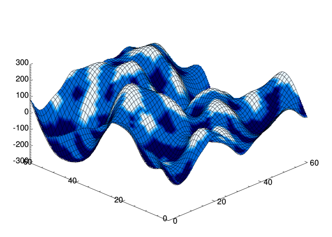
Figure 1: Example of location of “lake”, “hill” and “saddle” points in a Gaussian random field smoothed with a Gaussian window of size 5 pixels. The points are colored according to their type: “hill” points are in white, “lake” points in dark grey and “saddle” points in light grey. Lakes are connected to light grey hills by dark grey saddles. “Lake” and “hill”points are of comparable abundance while “saddle” points are the most common. The evolution of the relative abundances with thresholding can be well visualized from this plot: for example, when the threshold gets higher, the relative abundance of lake points decreases, while on the contrary the fraction of hill points increases, as expected. In this paper we shall rely on details of these variations to discriminate between a Gaussian and a non Gaussian random field.

This paper is organized as follows. In section § 2, after recalling some useful results about 2D Gaussian random fields, we derive analytic predictions for the abundances, by extending the work of Bond & Efstathiou (1987). In section § 3 we discuss technical issues involved in the practical measurements of ${\cal P}_{\rm hill}$, ${\cal P}_{\rm lake}$ and ${\cal P}_{\rm saddle}$. In section § 4 we build a $\chi^{2}$ statistic that allows us to combine a set of measurements in order to quantify the likelihood of an image to be Gaussian, from the standpoint of this measure. We then apply the method to the case of noisy mixed models involving cosmic strings plus cold dark matter. Finally, results are discussed in section § 5.

2 Theoretical Considerations

In this section we recall some specific properties of 2D Gaussian random fields, following Bond & Efstathiou (1987) (BE87) (a 2D transcription of the 3D formalism of Bardeen et al. 1986). We extend the calculations of this work to obtain theoretical expressions for the abundances of interest, i.e. the fractions of space occupied respectively by hill, lake and saddle regions.

2.1 Facts about a Gaussian random field

Let us first consider a temperature fluctuation field, $\delta_{\rm T}({\mathbf{r}})=T({\mathbf{r}})/\bar{T}-1$ whose $2D$ Fourier transform is $\delta_{\rm T}({\mathbf{k}})\equiv\int d^{2}{\mathbf{k}}\delta_{\rm T}({\mathbf{r}})\exp(i{\mathbf{k}.r})$ and whose power spectrum $P(k)$ is

$$\langle\delta_{\rm T}({\mathbf{k}})\delta_{\rm T}({\mathbf{k}^{\prime}})\rangle=(2\pi)^{2}P({\mathbf{k}})\delta_{D}({\mathbf{k}}+{\mathbf{k}^{\prime}}),$$ (1)

where $\delta_{D}({\mathbf{k}})$ is the Dirac distribution. We can define the moments of the power spectrum

$$\sigma_{j}^{2}\equiv{1\over(2\pi)^{2}}\int d^{2}{\mathbf{k}}\ P(k)k^{2j}$$ (2)

and the ratio

$$\gamma\equiv{\sigma_{1}^{2}\over\sigma_{0}\sigma_{2}}.$$ (3)

Note that $\sigma_{0}$ is the rms of the fluctuation field $\delta_{\rm T}$. Naturally, in the flat sky approximation, i.e. large multipole $l$ and small separation angles, the Fourier (flat) power spectrum is related to spherical harmonic power spectrum as follows

$$P(k)\simeq C_{\ell}\quad\mathrm{and}\quad k\simeq\ell.$$ (4)

Let us consider from now on only the normalized fluctuation field

$$\delta(\mathbf{x})\equiv{\delta_{\rm T}(\mathbf{x})\over\sigma_{0}}.$$ (5)

At a given point ${\mathbf{r}}$, we note the gradient of the field $\nabla\delta\equiv{\mathbf{\eta}}$ and the Hessian matrix, $\zeta_{ij}\equiv\partial\delta/\partial x_{i}\partial x_{j}$. This symmetric real matrix can be diagonalised by applying a rotation of an angle $\theta$ and we note $\lambda_{1}$ and $\lambda_{2}$ the opposite of its eigenvalues, with $\lambda_{1}\geq\lambda_{2}$. The normalized trace of the curvature matrix reads,

$$x\equiv{\lambda_{1}+\lambda_{2}\over\sigma_{2}},$$ (6)

and the ellipticity $e$ is defined as

$$e={\lambda_{1}-\lambda_{2}\over 2\sigma_{2}x}.$$ (7)

Note that with this notation, $x$ and $e$ should have the same sign. If $\lambda_{2}\geq 0$ then $x\geq 0$ and $0\leq e\leq 1/2$, if $\lambda_{1}\leq 0$ then $x\leq 0$ and $-1/2\leq e\leq 0$. If $\lambda_{1}$ and $\lambda_{2}$ have opposite signs, then neither $x$ nor $e$ are restricted.

For a Gaussian random field, the joint probability distribution function of $\delta$, ${\mathbf{\eta}}$, $x$, $e$ and $\theta$ is given by [Eq. (A1.6) in BE87]

$${\mathcal{P}}(\delta,{\mathbf{\eta}},x,e,\theta)d\delta\ dx\ de\ d\theta\ d^{2}{\mathbf{\eta}}=$$ (8)

$$e^{-\delta^{2}/2}{\mu d\delta\over\sqrt{2\pi}}e^{-\mu^{2}(x-\gamma\delta)^{2}/2}{dx\over\sqrt{2\pi}}\ \times$$

$$e^{-{\mathbf{\eta}}^{2}/\sigma_{1}^{2}}{d^{2}{\mathbf{\eta}}\over\pi\sigma_{1}^{2}}e^{-4x^{2}e^{2}}8x^{2}ede{d\theta\over\pi},$$

where we set

$$\mu\equiv(1-\gamma^{2})^{-1/2}.$$ (9)

Knowing this probability distribution function, it is easy to show that $\langle\delta^{2}\rangle=\langle x^{2}\rangle=\langle{\mathbf{\eta}}^{2}\rangle=1$, that ${\mathbf{\eta}}$ is correlated with neither $\delta$ nor $x$ nor $e$, but that $\langle\delta x\rangle=\gamma$, i.e. the height of a point is correlated with the curvature at this point. This lattest result is of particular interest to us since the so-induced non-trivial dependence on thresholding will generate a specific gaussian signature that we will exploit in the following.

2.2 Studying the local curvature

BE87 calculated the density probability of extrema for a Gaussian random field as a function of threshold. So using the properties of first derivatives, they open the way to further works [Heavens & Sheth 1999, Heavens & Gupta 2001] that illustrate the use of the number and spatial distribution of extrema to characterize Gaussian random fields.

We aim at extending this work to second derivatives by characterizing the local curvature at any point and then by comparing the abundance of $3$ defined types.

The local curvature is defined by the Hessian. By considering the sign of its eigenvalues ($-\lambda_{1}$ and $-\lambda_{2}$) we are led to distinguish three families of points :

• the “hill” points for which both eigenvalues are negative, i.e. $x\geq 0$ and $0\leq e\leq 1/2$;

• the “lake” points for which both eigenvalues are positive, i.e. $x\leq 0$ and $-1/2\leq e\leq 0$;

• the “saddle” points for which the eigenvalues are of different signs.

The first, second and third family incorporate respectively maxima, minima and saddle points.

Extending the calculation of BE87 we now compute the probability that a point ($\delta,{\mathbf{\eta}},x,e,\theta)$ above a given threshold $\delta_{\rm th}$, i.e. such that $\delta\geq\delta_{\rm th}$, belongs to any of these three classes. More precisely we calculate the quantities ${\mathcal{P}}_{\rm hill}(\delta_{\rm th})\equiv{\mathcal{P}}(0\leq x,0\leq e\leq 1/2|\delta_{\rm th}\leq\delta)$, ${\mathcal{P}}_{\rm lake}(\delta_{\rm th})\equiv{\mathcal{P}}(0\geq x,0\geq e\geq 1/2|\delta_{\rm th}\leq\delta)$ and ${\mathcal{P}}_{\rm saddle}(\delta_{\rm th})=1-{\mathcal{P}}_{\rm hill}(\delta_{\rm th})-{\mathcal{P}}_{\rm lake}(\delta_{\rm th})$.

To compute the quantity ${\mathcal{P}}_{\rm hill}(\delta_{\rm th})$ we first estimate the probability ${\mathcal{P}}(0\leq x,0\leq e\leq 1/2,\delta_{\rm th}\leq\delta)$. Starting from the distribution, Eq. (8), for the cases of interest to us, we can perform straightforwardly both the integration $\int_{-\infty}^{\infty}d^{2}{\mathbf{\eta}}/(\pi\sigma_{1}^{2})\displaystyle$ and $\int_{0}^{\pi}d\theta/\pi\displaystyle$. Doing so yields a probability function ${\mathcal{P}}(\delta,x,e)\displaystyle$. Note that the fact that $\theta\in[0,\pi]$ is due to the chosen ordering of the eigenvalues ($\lambda_{1}\geq\lambda_{2}$) implicit in the distribution Eq. (8). The subsequent integration $\int_{0}^{1/2}de\ \ \displaystyle$ yields the differential density

$${\mathcal{N}}_{\rm hill}(\delta,x,0\leq e\leq 1/2)\ d\delta dx\ =$$ (10)

$$\ e^{-\delta^{2}/2}\ {\mu d\delta\over(2\pi)^{1/2}}e^{-\mu^{2}(x-\gamma\delta)^{2}/2}(1-e^{-x^{2}}){dx\over(2\pi)^{1/2}}.$$

Then we can still perform analytically the integration over $x\geq 0$ and we get

$${\mathcal{N}}_{\rm hill}(\delta,0\leq x,0\leq e\leq 1/2)d\delta\ \ =$$ (11)

$$e^{-\delta^{2}/2}\ {\mu d\delta\over 2\sqrt{2\pi}}\ \Bigl{[}\ {1\over\mu}\ \Bigl{(}1+\mathrm{Erf}\Bigl{(}{\gamma\mu\delta\over\sqrt{2}}\Bigr{)}\ \Bigl{)}-$$

$${e^{-\mu^{2}\gamma^{2}\delta^{2}/(2+\mu^{2})}\over\sqrt{2+\mu^{2}}}\Bigr{(}1+\mathrm{Erf}\Bigl{(}{\gamma\mu^{2}\delta\over\sqrt{2}\sqrt{2+\mu^{2}}}\Bigr{)}\ \Bigr{)}\ \Bigr{]}.$$

The integration over some threshold $\delta_{\rm th}$ cannot be performed analytically. However, knowing that

$${\mathcal{P}}(\delta_{\rm th}\leq\delta)={1\over 2}\mathrm{Erfc}\left({\delta_{\rm th}\over\sqrt{2}}\right)\;,$$ (12)

it is easy to evaluate numerically the quantity

$${\mathcal{P}}_{\rm hill}(\delta_{\rm th})={\int_{\delta_{\rm th}}^{\infty}\ {\mathcal{N}}_{\rm hill}(\delta,0\leq x,0\leq e\leq 1/2)d\delta\over{\mathcal{P}}(\delta_{\rm th}\leq\delta)}.$$ (13)

We can still obtain analytically the limiting value ${\mathcal{P}}_{\rm hill}(\delta_{\rm th}=-\infty)$, i.e. the fraction of “hill” points in the absence of threshold. We find

$${\mathcal{P}}_{\rm hill}(\delta_{\rm th}=-\infty)={1\over 2}\left(1-{1\over\sqrt{3}}\right)\simeq 0.2113\;.$$ (14)

An analogous calculation can be performed for “lake” points. It leads to the differential density

$${\mathcal{N}}_{\rm lake}(\delta,x\leq 0,-1/2\leq e\leq 0)d\delta\ \ =$$ (15)

$$e^{-\delta^{2}/2}\ {\mu d\delta\over 2\sqrt{2\pi}}\ \Bigl{[}\ {1\over\mu}\ \mathrm{Erfc}\Bigl{(}{\gamma\mu\delta\over\sqrt{2}}\ \Bigl{)}\ -\$$

$${e^{-\mu^{2}\gamma^{2}\delta^{2}/(2+\mu^{2})}\over\sqrt{2+\mu^{2}}}\mathrm{Erfc}\Bigl{(}{\gamma\mu^{2}\delta\over\sqrt{2}\sqrt{2+\mu^{2}}}\Bigr{)}\ \Bigr{]}$$

from which we can deduce numerically ${\mathcal{P}}_{\rm lake}(\delta_{\rm th})$ as in Eq. (13). The asymptotic value ${\mathcal{P}}_{\rm lake}(\delta_{\rm th}=-\infty)$ can also be obtained analytically, and from parity argument one finds

$${\mathcal{P}}_{\rm lake}(\delta_{\rm th}=-\infty) = {\mathcal{P}}_{\rm hill}(\delta_{\rm th}=-\infty)$$

$$= {1\over 2}(1-{1\over\sqrt{3}})\simeq 0.2113.$$

Two remarkable properties of Gaussian random fields emerge from the above analytical calculations:

• the evolution of the “hill”, “lake” and “saddle” point fractions as functions of threshold $\delta_{\rm th}$ depends only on the spectral parameter $\gamma$;

• the asymptotic value for $\delta_{\rm th}\rightarrow-\infty$ is independent of any spectral parameter, i.e. is the same for any Gaussian random field. This would not be true if we were considering only maxima, minima or saddle points (see BE87).

To illustrate these results, we draw on Fig. 2 the functions ${\mathcal{P}}_{\rm lake}(\delta_{\rm th})$ and ${\mathcal{P}}_{\rm hill}(\delta_{\rm th})$ for a set of $\gamma$ values. Except in the limit $\delta_{\rm th}\rightarrow-\infty$, the evolution of these functions with $\delta_{\rm th}$ is rather sensitive to $\gamma$.

At this point, it is important to be aware that till now, we have supposed an idealistic, infinite resolution experiment, i.e. we did not take into account any beam smearing effect that would affect any real measurement. Consequently, in order to compare the predictions to any true measurements, it would be necessary to incorporate this effect in our calculations. To do so, we should consider the convolved field, $\delta\ast B$, where $B$ stands for the instrumental beam response, instead of the idealistic fluctuation field, $\delta$. Since linear transformations such as the convolution by an arbitrary beam function do not change the Gaussian nature of a random field, the beam smearing should appear only as a dependence of $\gamma$ on the smoothing scale $\sigma_{\rm b}$, that we will note $\gamma(\sigma_{\rm b})$. Furthermore, although the problem of beam convolution in its full generality is very intricate, it turns out to be analytically tractable for a Gaussian, symmetric beam, a reasonable approximation in practice. We will illustrate this point in more details below.

Figure 2: Functions ${\mathcal{P}}_{\rm hill}(\delta_{\rm th})$ and ${\mathcal{P}}_{\rm lake}(\delta_{\rm th})$ in the Gaussian case for various values of $\gamma$ as indicated on the figure. Their value is independent of $\gamma$ in the limit $\delta_{\rm th}\rightarrow-\infty$, but their evolution with $\delta_{\rm th}$ is rather sensitive to $\gamma$. Similar conclusions hold for function ${\mathcal{P}}_{\rm saddle}(\delta_{\rm th})=1-{\mathcal{P}}_{\rm hill}(\delta_{\rm th})-{\mathcal{P}}_{\rm lake}(\delta_{\rm th})$, which is not plotted for simplicity.

3 Confronting Predictions and Measurements on Simulations

In order to test our ability to measure the functions ${\mathcal{P}}_{\rm hill}(\delta_{\rm th})$ and ${\mathcal{P}}_{\rm lake}(\delta_{\rm th})$, and to measure the incertainties for maps of limited extent, we performed several measurements on simulated maps. We henceforth limit ourselves to small simulated square patches of the sky of width $\sim 12.5\ \mathrm{deg}$. These patches are considered as being flat and pixelized with a $512\times 512$ Cartesian mesh of resolution $\theta_{\rm pix}=1.5^{\prime}$.

This section is organized as follows: we first describe the measurement principles (§ 3.1) and apply them to noise free realization of Cold Dark Matter (CDM) ($\Omega_{m}=0.3$, $\Omega_{\Lambda}=0.7$, $h=0.5$, $\Omega_{b}=0.05$ and $n=1$) Gaussian maps generated from their power spectrum (taking into account both the uniform distribution of the phases of the Fourier modes and the Rayleigh distribution of their modulus) (§ 3.2); in particular, we examine the Gaussianity of the distribution function of measurements in order to be able to perform later $\chi^{2}$ tests; finally we discuss practical issues related to finite resolution and finite volume effects (§ 3.3).

Figure 3: Measurement of functions ${\mathcal{P}}_{\rm hill}$ and ${\mathcal{P}}_{\rm lake}$ on Gaussian simulated maps in the standard CDM case. The triangles and the losanges give respectively the hill and lake point fractions obtained from an average over 200 realizations of size $12.5\times 12.5\ \mathrm{deg}^{2}$. The error bars on each symbol are obtained from the dispersion over the 200 realizations. Prior to measurement, a smoothing with a Gaussian window of size $\sigma_{\rm b}=5\theta_{\rm pix}$ was performed. The continuous and dashed curves correspond to the theoretical expectations for a Gaussian random field with $\gamma_{\rm eff}=0.48$.

3.1 Principles of measurements

The measurements consist in determining the fractions ${\mathcal{P}}_{\rm hill}$ and ${\mathcal{P}}_{\rm lake}$ for an ensemble of excursion sets (subsets for which $\delta\geq\delta_{\rm th}$) of an image smoothed at different scales $\sigma_{\rm b}$. To insure sufficient differentiability, i.e. at least continuity of second order derivatives, we choose a Gaussian smoothing window.

Similarly as in Colombi et al. (2000) for the 3D case, to measure the local curvature at a given point, we find the quadratic form which fits this point and its $8$ closest neighbors. We deduce from the quadratic form coefficients the local values of the second derivatives, i.e. the Hessian matrix, then diagonalize this matrix and determine the sign of its eigenvalues $\lambda_{1}$ and $\lambda_{2}$. Both easy to implement and fast, this method turns out to be quite robust in the presence of noise.

3.2 Example: application to noise free realizations

As a first example, we apply this measurement technique to $200$ simulated noise free realizations of CDM like temperature maps smoothed by a Gaussian beam of $\sigma_{\rm b}=5\theta_{\rm pix}=7.5^{\prime}$. In each realization, we measure both ${\mathcal{P}}_{\rm hill}(\delta_{\rm th})$ and ${\mathcal{P}}_{\rm lake}(\delta_{\rm th})$ for the ensemble of excursion sets defined by $\delta_{\rm th}=-3.0$, $-2.5$, $-2.0\ldots 3.0$, as illustrated by Fig. 3. For comparison purpose, we plotted on this figure the theoretical curves corresponding to the expected value of the parameter $\gamma(\sigma_{\rm b}=5^{\prime})=0.48$. This effective $\gamma$ can be easily calculated for a Gaussian beam, since in this context we just have to replace $P(k)$ (an exact theoretical input here) by $P(k)\exp(-k^{2}\sigma_{\rm b}^{2})$ in Eqs. (2) and (3), (see Fig. 6 and section § 3.3 for a mode detailled illustration of this calculation). With this choice of $\gamma$, the theoretical curves fit very well the data. The dispersion over the measurements is very tight except at high threshold where we enter a rare events regime, as indicated by the larger $1\sigma$ error bars.

To illustrate more visually the protocol, Fig. 5 displays one CDM realization (noise free again) smoothed at $\sigma_{\rm b}=3\theta_{\rm pix}$, the corresponding excursion set for $\delta\geq 1$ as well as the local curvature map, where $hill$, $lake$ and $saddle$ points are identified by respectively black, white and grey points. A cross examination of these images provides some insight on the processe involved, i.e. the correlation of extrema and local curvature.

To further investigate the dispersion over the measured values of ${\mathcal{P}}_{\rm hill}(\delta_{\rm th})$ at a given $\delta_{\rm th}$, we drawn on Fig. 4 the probability distribution function of the hill point fraction measured from the 200 realizations [similar results can be obtained for ${\mathcal{P}}_{\rm lake}(\delta_{\rm th})$]. Two thresholds are considered, $\delta_{\rm th}=-2$ (left pannel) and $\delta_{\rm th}=0$ (right pannel). The dashed line on each pannel corresponds to the Gaussian limit with same standard deviation as the one actually measured. It fits qualitatively well the measurements, so the previously drawn $1\,\sigma$ errors are meaningful estimates of the cosmic variance errors. We checked wether the distribution function of the measurements is Gaussian for other values of $\delta_{\rm th}$ and found that it is indeed the case except at high threshold, $\delta_{\rm th}\geq 2.5$, where one enters the rare events regime.

Figure 4: Distribution function of hill points fraction obtained from 200 CDM noise free realizations of temperature maps smoothed with a gaussian window of size $\sigma_{\rm b}=3\theta_{\rm pix}$, similarly as in Fig. 5. Two excursion sets are considered, one with $\delta_{\rm th}=-2$ (left panel) and the other one with $\delta_{\rm th}=0$ (right panel). The smooth dotted-dashed curve on each panel corresponds to a Gaussian of same variance as the distribution function. It superposes well to the measurements (histograms) for the excursion sets considered here.

Thus, the measurements in this idealistic noise free case are in very good agreement with theoretical expectations. Furthermore, the cosmic errors associated with these measurements are very tight for a Gaussian field. This last point will be of particular interest to us since it makes the evolution of functions ${\mathcal{P}}_{\rm hill}(\delta_{\rm th})$ and ${\mathcal{P}}_{\rm lake}(\delta_{\rm th})$ with $\delta_{\rm th}$ a sharp signature of random Gaussian fields.

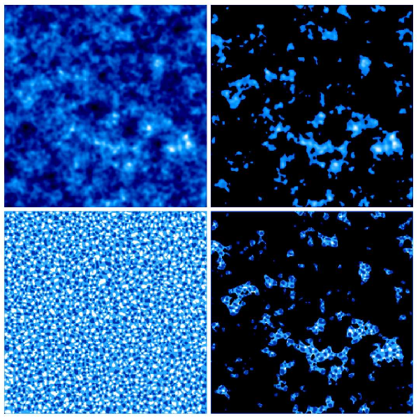
Figure 5: Illustration of the measurement protocol. Considering a CDM temperature map with $512\times 512$ pixels, of width $12.5\ \mathrm{deg}\times 12.5\ \mathrm{deg}$ and smoothed with a Gaussian window of size 3 pixels (top left panel), we identify “hill”, “lake”and “saddle” points according to their local curvature (respectively by dark grey, white and light grey points on the bottom left panel). The fraction of space occupied by each kind of point is studied as a function of the density threshold. As an example, the excursion set corresponding to $\delta_{\rm th}=1$ is shown in right pannels, which are the same than left panels except that only regions with $\delta\geq\delta_{\rm th}$ are shown, the rest being coded in black. As one can see, the relative abundance of “lake” points in bottom right panel is now smaller than on bottom left panel, while which of “hill” points has augmented, as expected. The measurement of the relative fraction of the three kind of points as a function of density threshold is the key idea of this paper.

3.3 Measuring $\gamma$: spurious effects and available dynamic range

In the above discussion, we used a predicted value of $\gamma$ to check if the measured “hill”, “saddle” and “lake” point fractions agreed with theoretical predictions for a Gaussian random field. Therefore, the only thing we proved so far is that for a finite realization of a Gaussian random field smoothed with a Gaussian of width $\sigma_{\rm b}=3\theta_{\rm pix}$, whose (unsmoothed) power spectrum is perfectly known, the predicted value $\gamma$ agrees very well with the measured points. In practice however, the knowledge of the power spectrum might be less accurate and we want to develop a non-Gaussianity test which can be performed both independently or in combination with the power spectrum measurement. Thus it is important to determine from the measurements of these fractions themselves an effective value, $\gamma_{\rm eff}$, that fits well the data. We will see that for a finite realization of a Gaussian random field, there always exists a value $\gamma_{\rm eff}$ which is such that measurements agree very well with analytic predictions.

As we shall see below, the determination of the $\gamma_{\rm eff}$ value is easy and this fact, by itself, is highly significant and is the key point of our paper: for a map in which temperature fluctuations are partly seeded by cosmic strings, we shall see that it is actually not possible to find a value of $\gamma_{\rm eff}$ leading to point fractions matching the measurements in all the available dynamic range – namely, for all possible values of $\delta_{\rm th}$ and $\sigma_{\rm b}$. However, as we shall see later, it is not needed to accurately determine the real value of $\gamma$ to efficiently constrain the level of non Gaussianity of a map.

However, studying the difference between $\gamma$ and $\gamma_{\rm eff}$ can help to determine the available dynamic range, i.e. the set of values of $\delta_{\rm th}$ and $\sigma_{\rm b}$ in which one can trust the measurements. We already noticed in previous section that the density threshold should be small enough, $\delta_{\rm th}\la 2.5$, to avoid entering the rare event regime, where the cosmic distribution function of measurements becomes non Gaussian. Here, we are concerned by two effects that we ignored previously:

• Pixelization effects, or equivalently, effects of finite resolution: as discussed above, it is important to smooth the data to insure sufficient differentiability. The smoothing scale should be large enough compared to the pixel size to avoid anisotropies or discreteness effects brought by the pixelization.

• Finite volume and edge effects: our experimental maps cover a rather small fraction of the sky, due to the limited dynamical range in the cosmic-string simulations from [Bouchet et al. 1988, Bennett & Bouchet 1990]. Therefore, to avoid reducing too much the number of statistically independent regions of the map, the smoothing scale should not be too large. In a more realistic experiment covering a large fraction of the sky, finite volume and edge effects should not be as much as of a concern.

The practical measurement of $\gamma_{\rm eff}$ is made straightfoward by noticing that the dependence of the function $\tilde{\mathcal{P}}_{\rm hill}(\delta_{\rm th}=1)$ on $\gamma$ is very well approximated by an exponential law in the domain of interest to us, i.e. $0.4\leq\gamma\leq 0.95$: the fit

$$\ln\tilde{\mathcal{P}}_{\rm hill}(\delta_{\rm th}=1)\simeq a+b\gamma$$ (17)

with $a=-1.4099$ and $b=1.2395$ is accurate to $0.6\%$. The choice of the particular value $\delta_{\rm th}=1$ is an ad hoc compromise coming from the competition between two effects: (i) the dependence on $\gamma$ of the quantity $\tilde{\mathcal{P}}_{\rm hill}(\delta_{\rm th})$ increases with $\delta_{\rm th}$ (Fig. 2), but (ii) the uncertainty on the determination of $\tilde{\mathcal{P}}_{\rm hill}(\delta_{\rm th})$ increases with $\delta_{\rm th}$ (Fig. 3).

To test the effects of finite coverage and finite resolution, we examine a CDM case, where we generated once again some Gaussian field realisations from their $C_{\ell}$. Assuming as before that the field has been smoothed by a Gaussian of width $\sigma_{\rm b}$, we can easily compute the prediction for the function $\gamma(\sigma_{\rm b})$.

In Fig. 6, the measured values of $\gamma_{\rm eff}$ is displayed in each case as a function of smoothing scale. An average over 50 realizations of $512\times 512$ pixels maps is performed. The error bars on the figure represent the corresponding scatter, which increases with $\sigma_{\rm b}$ as expected, due to finite volume effects. The solid line corresponds to the theoretical function $\gamma(\sigma_{\rm b})$. Agreement between $\gamma_{\rm eff}$ and the analytic prediction is good, except at small scales where pixelisation effects contaminate this measurements. We however see that pixelisation effects become negligible when $\sigma_{\rm b}/\theta_{\rm pix}>3$. Note that there should be an upper bound as well for $\sigma_{\rm b}$ as discussed above, since cosmic errors increase with scale. Our $\chi^{2}$ analysis below will anyway naturally take that into account by giving a lesser weight to scales with larger errors. This reasonable agreement between the measured $\gamma_{\rm eff}$ at a given scale $\sigma_{\rm b}$ and the expected $\gamma(\sigma_{\rm b})$ validates the approach we will use in the next section which consists in finding from the fraction themselves an ad hoc $\gamma_{\rm eff}$, and deducing from it an agreement with Gaussianity.

Figure 6: Measurement of $\gamma_{\rm eff}$ as a function of the smoothing scale $\sigma_{\rm b}/\theta_{\rm pix}$. The solid line gives the theoretical values of $\gamma$ for various $\sigma_{\rm b}$. They were computed using the power spectrum $C_{\ell}$. The crosses with error bars correspond to measurements of $\gamma_{\rm eff}$ using the measurements of ${\cal P}_{\rm hill}(\delta_{\rm th}=1.0)$. The error bars correpond to $\pm 1$ the measured rms on 50 realisations. Pixelisation effects bias the measurements of $\gamma_{\rm eff}$ till $\sigma_{\rm b}/\theta_{\rm pix}=3$. The error bars grows with $\sigma_{\rm b}$ as expected from sampling variance arguments.

4 Testing Non-Gaussianity : Principle and Application to Mixed Models

¿From the previous section, we conclude that in the case of a smoothed Gaussian random field, the functions ${\cal P}_{\rm hill}(\delta_{\rm th})$ and ${\cal P}_{\rm void}(\delta_{\rm th})$ can be measured accurately and fit very well the analytical predictions provided $\gamma$ be considered as an adjustable parameter. Furthermore, their probability distribution function is well approximated by a Gaussian if $\delta_{\rm th}\la 2.5$, which now allows us to define a rigorous measurement protocol based on $\chi^{2}$ analysis that we shall apply to simulated data in the trustable scale range determined above, namely $\sigma_{\rm b}\geq 3$.

In this section, we first detail how we use the functions ${\cal P}_{\rm hill}(\delta_{\rm th})$ and ${\cal P}_{\rm void}(\delta_{\rm th})$ to build a $\chi^{2}$ statistic testing Gaussianity (§ 4.1). Then we apply the method to simple simulated mixed models involving cosmic strings plus CDM and see how it can be used to bound quantitatively the relative contribution of cosmic strings (§ 4.2).

4.1 The method

Let us assume as before that we have at our disposal an observed temperature map $\delta_{\rm T}$, on which we measured the fractions ${\mathcal{P}}_{\rm hill}(\delta_{\rm th_{i}},\sigma_{\rm b_{i}})$ and ${\mathcal{P}}_{\rm lake}(\delta_{\rm th_{i}},\sigma_{\rm b_{i}})$ for a set of threshold values $\{\delta_{\rm th_{i}}\}$ and smoothing scales $\{\sigma_{\rm b_{i}}\}$. If the power spectrum of this random field is known, we can in principle define analytically a set of values of $\gamma$ for each smoothing scale, $\{\gamma_{\sigma_{\rm b_{i}}}\}$. Assuming furthermore that the field is Gaussian and that our estimators of ${\mathcal{P}}_{\rm hill}$ and ${\mathcal{P}}_{\rm lake}$ are unbiased, it is easy to deduce from this $\gamma$ set some theoretical expectations for the set, $\tilde{\mathcal{P}}_{\rm X}(\delta_{\rm th_{i}},\sigma_{\rm b_{i}})\equiv\langle{\mathcal{P}}_{\rm X}(\delta_{\rm th_{i}},\sigma_{\rm b_{i}})\rangle$, where ${\rm X}$ stands from now on for “lake” or “hill”. To quantify the distance between these theoretical predictions and the measurements, we introduce the standard $\chi^{2}$ statistic. Since these measurements can obviously not be considered as independent, we have to introduce the full theoretical variance-covariance matrix

$$C_{\rm II^{\prime}}\equiv\langle({\mathcal{P}}_{\rm I}-\tilde{\mathcal{P}}_{\rm I})({\mathcal{P}}_{\rm I^{\prime}}-\tilde{\mathcal{P}}_{\rm I^{\prime}})\rangle,$$ (18)

where we use the short hand notation ${\cal P}_{\rm I}={\mathcal{P}}_{\rm X}(\delta_{\rm th_{i}},\sigma_{\rm b_{i}})$ and ${\cal P}_{\rm I^{\prime}}={\mathcal{P}}_{\rm X^{\prime}}(\delta_{\rm th_{i^{\prime}}},\sigma_{{\rm B_{i^{\prime}}}})$. Then, the statistic

$$\chi^{2}\equiv\sum_{\rm II^{\prime}}\ ({\mathcal{P}}_{\rm I}-\tilde{{\mathcal{P}}}_{\rm I})\ (C_{\rm II^{\prime}})^{-1}\ ({\mathcal{P}}_{\rm I^{\prime}}-\tilde{{\mathcal{P}}}_{\rm I^{\prime}})\ .$$ (19)

is expected to follow a $\chi^{2}$-distribution, as illustrated by a practical example below. Indeed results of § 3.2 suggest that the distribution function of the measured ${\mathcal{P}}_{\rm I}$ is nearly Gaussian if $\delta_{\rm th}\la 2.5$.

In practice, we have to introduce two more subtleties in this protocol.

First, as discussed extensively in § 3.3, the practical realization of a Gaussian random field yields a measured function ${\mathcal{P}}_{\rm I}$ matching the theory, $\tilde{\mathcal{P}}$, but with an effective value of $\gamma$. Taking into account some additional Gaussian noise, as discussed in more details below, would make this effect even stronger. Rigorously, we should modelize this $\gamma_{\rm eff}$ effect in terms of statistical bias on the estimators of the function ${\mathcal{P}}_{\rm X}(\delta_{\rm th},\sigma_{\rm b})$, but we proceed here differently, for simplicity: we extract the $\gamma_{\rm eff}(\sigma_{\rm b})$ from the data by fitting the analytic prediction for function ${\mathcal{P}}_{\rm hill}(\delta_{\rm th}=1,\sigma_{\rm b})$ to the measured one. Thus, our “theory” depends itself on the data through $\gamma_{\rm eff}$. As already explained, the critical test for non Gaussianity will be on the evolution of the functions ${\mathcal{P}}_{\rm X}(\delta_{\rm th},\sigma_{\rm b})$ with $\delta_{\rm th}$, which, once $\gamma_{\rm eff}$ is determined, is entirely fixed. The practical measurement of $\gamma_{\rm eff}$ is performed as explained in the previous section. In principle we could include the value of $\delta_{\rm th}$ used to measure $\gamma_{\rm eff}$ as a varying parameter in our $\chi^{2}$ test, to optimize the analysis. Given the level of accuracy of our numerical experiments and since we just aim here to illustrate the method in a simple and convincing way, we did not feel necessary to do so.

Second, even if in principle we could compute analytically or numerically the variance-covariance matrix, for the sake of simplicity we evaluated it using a Monte-Carlo method based on a few hundreds of Gaussian realizations having the same power-spectrum and noise properties as the input map. So for each model we will consider below (pure CDM, mixed model with CDM + cosmic strings, and pure cosmic strings), the covariance matrix $C$ should be different in each case. However, in practice we checked that this matrix coefficients depend very slightly on $\gamma_{\rm eff}$ in the range of interest to us, i.e. $0.4\leq\gamma\leq 0.95$ so that we consider for simplicity only the same $C$ matrix in each case. Another issue concerning this matrix is that it might be singular. Indeed, since fractions measured at various thresholds and different scales can be highly correlated, e.g. the values at very low threshold where the dependence on $\gamma$ is very weak, the studied $\{\delta_{\rm th_{i}}\}$ and $\{\sigma_{\rm b_{i}}\}$ sets have to be restricted so that $C$ is invertible.

4.2 Application on mixed models for MAP and Planck

As an illustration of the accuracy of our statistics, we apply it in the framework of MAP and Planck Surveyor experiments to a mixed model where temperature fluctations are seeded in part by cosmic strings and otherwise by adiabatic inflationary perturbations in standard CDM model (e.g. Bouchet et al. 2001 and references therein). Our approach is rather simple, since we add together a CDM map and a temperature fluctuation map obained from ray-tracing in cosmic string simulations [Bouchet et al. 1988, Bennett & Bouchet 1990] and neglect possible cross-correlations between such maps. This implicitely supposes the existence of a standard CDM inflationary epoch followed by a phase transition during which cosmic strings appear and then imprint supplementary fluctuations on the dark matter distribution. Neglecting cross-correlations mentionned just above is equivalent to assume that the distribution of cosmic string as well as their dynamical evolution is not coupled with that of cold dark matter, which should be a good assumption at the level of approximation considered in this paper [Linde & Riotto 1997, Contaldi et al. 2001]. We neglect also any contribution to the fluctuations prior to the last scattering surface (lss) so that the comparaison with results from Bouchet et al. 2001, who considered this contribution, is not immediate at small scales.

To take into account the noise expected in the best channels of MAP and Planck Surveyor experiments (respectively $12.8\ \mathrm{\mu K/K}$ per $0.3\times 0.3\ \mathrm{deg}^{2}$ pixels and $2\ \mathrm{\mu K/K}$ per $8^{\prime}\times 8^{\prime}\ \mathrm{deg}^{2}$), we add an extra Gaussian white noise $n$ to our square maps. Note again, that as long as the noise is Gaussian, its presence can be simply taken into account by a change in the value of $\gamma_{\rm eff}$. Thus, our simulated temperature maps read

$$\delta_{\rm T}=(1-\beta)\ \delta_{\rm T}^{\rm string}+\beta\ \delta_{\rm T}^{\rm CDM}+n,$$ (20)

where $1-\beta$ represents the fraction of the signal seeded by cosmic strings, given the fact that we impose ${\rm rms}(\delta_{\rm T}^{string}\ )={\rm rms}(\delta_{\rm T}^{CDM})={\rm rms}(\delta_{\rm T}^{COBE}\ )$ for the fields smoothed at a scale corresponding to the COBE-DMR beam, i.e. $\sigma_{\rm b}=7^{\circ}/\sqrt{8\ln 2}$. Note that we differ from Bouchet et al. 2001 in the relative normalisation of the two contributions since they define their relative normalisation with $C_{\ell}$, i.e. they considered a family of models parametrized by $C_{\ell}=(1-\alpha)\ C_{\ell}^{\rm string}+\alpha\ C_{\ell}^{\rm CDM}\displaystyle$, where both $C_{\ell}^{\rm string}$ and $C_{\ell}^{\rm CDM}$ are COBE normalised and where $C_{\ell}^{\rm string}$ includes contributions from before and after the lss. If we wanted however to express our results, in terms of $\beta$, we should consider $1-\alpha=(1-\beta)^{2}/((1-\beta)^{2}+\beta^{2})$.

We now construct the previously defined $\chi^{2}$ statistics for various values of $\beta$ and try to figure out what is the smallest “string like contribution” that our method should be able to detect with a high statistical significance.

4.2.1 Constructing the $\chi^{2}$ and adequacy of the $\chi^{2}$ probability distribution

Figure 7: Histogram of the measured probability distribution of the quantity $\chi^{2}$ defined by Eq. (19), from $300$ noisy (Planck best channel noise level) realizations of CDM temperature fluctuations. The dot-dashed curve corresponds to a $\chi^{2}$-distribution with $47$ degrees of freedom (dashed line). The good agreement allows us to use $\chi^{2}$ as a measure of the Gaussian nature of the observed field.

Even if one would like to include as many threshold values and smoothing scales as possible in the analysis, this is in practice not necessary. Indeed, some measurements are, at least in the Gaussian case, highly correlated with each other, due to e.g. some strong constraints (in the very low threshold regime, $\delta_{\rm th}\rightarrow-\infty$, both ${\mathcal{P}}_{\rm lake}(\delta_{\rm th})$ and ${\mathcal{P}}_{\rm hill}(\delta_{\rm th})$ tend to an asymptotic value independent of the spectral parameters). Therefore, one can restrict the set of values of $(\sigma_{B},\delta_{\rm th})$ by requiring that the $C$ matrix (see Eq.18) be non-singular.

By investigating the numerical properties of $C$, we find for all the maps that $\delta_{\rm th}=-2$,$-1.5\ldots$, $+1.5$ and $\sigma_{\rm b}/\theta_{\rm pix}=6$, $10$ and $14$ (corresponding to repectively $21^{\prime}$, $35^{\prime}$ and $49^{\prime}$ on the sky) are satisfying values for the Planck case, whereas $\delta_{\rm th}=-1.5$,$-1.0\ldots$, $+1.5$ and $\sigma_{\rm b}/\theta_{\rm pix}=8$ and $12$ (corresponding to respectively $28^{\prime}$ and $42^{\prime}$) are reasonable for MAP. Of course, this choice of the set of values of $(\sigma_{B},\delta_{\rm th})$ is strongly influenced by the fact that our map is rather small: for a full sky survey, the sampling would probably be different.

Given these restrictions, it is now important to explore the properties of the probability distribution function of the $\chi^{2}$ statistics defined in Eq. (19). As stated previously, we expect it to follow a $\chi^{2}$-distribution, at least in the Gaussian case, since the distribution of measured values of ${\mathcal{P}}_{I}$s is well described by a Gaussian (see § 3.1). We tested this by generating 300 realizations of noisy (Planck level) CDM like only temperature fluctuations for which we measure $\chi^{2}$. Its probability distribution is drawn on Fig. 7, where we superimposed a theoretical $\chi^{2}$-distribution with $47$ degrees of freedom (dof) ($48$ measurements: $6\times 4$ measured hill points fraction and $6\times 4$ measured void point fractions; $1$ parameter, $\gamma$). The agreement is obviously very good, comforting the analysis procedure and making this $\chi^{2}$ statistic adequate for assessing Non-Gaussianity.

4.2.2 Ability to distinguish a “Non-Gaussianity Level” with a realistic noise level

Figure 8: Measurement of hill and lake point fractions in a Planck simulation with pure CDM ($\beta=1.0$). The left column shows the measured evolution of ${\mathcal{P}}_{\rm lake}$ as a function of threshold, $\delta_{\rm th}$, for two smoothing scales: top left panel corresponds to $\sigma_{\rm b}/\theta_{\rm pix}=10$ and bottom left panel to $\sigma_{\rm b}/\theta_{\rm pix}=14$. Symbols without error bars represent the measurements in the realization, while symbols with errorbars correspond to the Gaussian prediction matching the value of ${\mathcal{P}}_{\rm hill}(\delta_{\rm th}=1)$ as explained more in detail in § 4.1. The error bars are obtained from the 1-$\sigma$ dispersion over 300 realizations. The right column of panels is similar to left column, but for ${\mathcal{P}}_{\rm hill}$.

Making use of this $\chi^{2}$ statistics, we are now in position to determine how well we can distinguish non-Gaussian signatures.

Figure 9: Same as Fig. 8 but for the an hybrid model with $\beta=0.3$.

Figure 10: Same as Fig. 8 but for the pure string model ($\beta=0.0$).

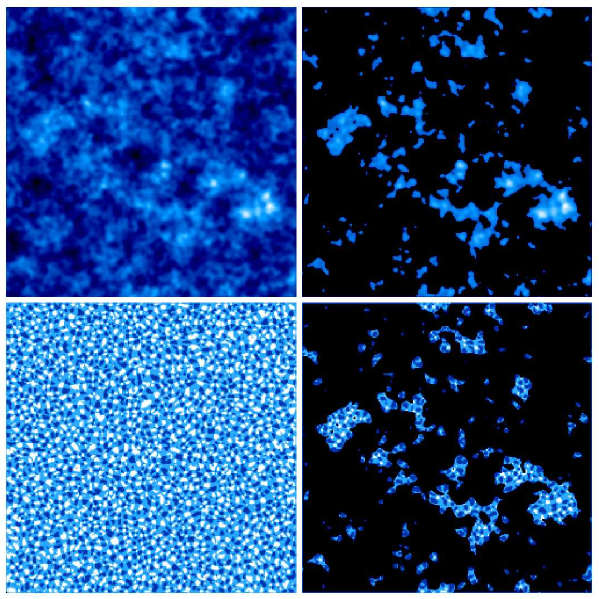
Figure 11: Same as in Fig. 5 but for a noise free mixed model with $\beta=0.7$. Note how difficult it is to distinguish it from the mere CDM map.

In Figs. 8, 10 and 10, we display some measurements of functions ${\mathcal{P}}_{\rm lake}(\delta_{\rm th})$ and ${\mathcal{P}}_{\rm hill}(\delta_{\rm th})$ in the Planck case. Three values of $\beta$ are considered: pure CDM with $\beta=1$, hybrid model with $\beta=0.3$ and pure string model with $\beta=0$. Again, On each figure, the Gaussian limit obtained from the procedure explained in detail in § 4.1 is compared to the measurements. The error bars on the theoretical predictions correspond to then the $1\sigma$ dispersion over 300 realizations of pure random Gaussian fields with same power-spectrum and noise properties as the data, as explained in end of § 4.1. Very good agreement is found for CDM, as expected, while the hydrid model exhibits some discrepancies, especially for ${\cal P}_{\rm lake}$. These discrepancies are overwhelming in the string only model. Note that since we fit the measured value of ${\mathcal{P}}_{\rm hill}(\delta_{\rm th}=1)$ to estimate the Gaussian prediction, one expects non Gaussian features to show up more in the measured shape of function ${\cal P}_{\rm lake}(\delta_{\rm th})$ than that of function ${\mathcal{P}}_{\rm hill}(\delta_{\rm th})$, as indeed seen at least for the mixed model. Note also that if for the mixed model, the measured ${\cal P}_{\rm lake}(\delta_{\rm th})$ tends to lie below the Gaussian prediction, the reverse happens for the pure string model (this seemingly counterintuitive result stems from our comparing the data to a “theoretical” curve which is different in the 2 cases) . Finally, it is important as well to recall that data points plotted on Figs. 8–10 represent only 2/3 of all the points used for the $\chi^{2}$ computation since we consider one more smoothing scale, $\sigma_{\rm b}/\theta_{\rm pix}=6$.

To illustrate more qualitatively these measurements, Figures 11 and 13 display, similarly as in Fig. 5, an example of initial smoothed noise free map, its thresholded counterpart (with $\delta_{\rm th}=1$) and the corresponding local curvature maps with lake, saddle and hill points. Figure 11 corresponds to the hybrid model case ($\beta=0.3$) while Figure 13 corresponds to the string only model ($\beta=0.0$). A strong similarity can be seen between the mere CDM and the hybrid models despite the differences in measured ${\cal P}_{\rm lake}$ functions. Note also the peculiar patterns in the pure string curvature map: there seem to be rather extended saddle point regions, which calls for other specific pattern detection statistics.

Table 1 summarizes the results obtained for $\chi^{2}$ using the noise level of the best channel of either Planck or MAP. It shows, for various values of $\beta$, the measured $\chi^{2}$, the $\chi^{2}$ per dof, as well as the probability (noted Prob.) that a random variable, in a $\chi^{2}$-distribution with the relevant (number of) dof (shown above to be adequate) is greater than the obtained $\chi^{2}$. This quantity gives therefore the significance of the detection.

Roughly speaking, the smaller the $\chi^{2}$, the better is the agreement with a Gaussian distribution. Reversely, the higher the obtained $\chi^{2}$, the more unlikely does the analyzed map follow a Gaussian distribution.

Note that the numbers displayed in Table 1 represent in no way the best Planck and MAP can provide with our method, since we only considered 0.3% of the sky for one single channel. Nevertheless, these figures give some trends of the ability of our method, the purpose of this paper.

With these limitations in mind, we see that MAP can get a meaningful detection (1% level) of the non-Gaussianity induced by string like background with $\beta=0.7$, corresponding to a number $1-\alpha=0.15$, a number slightly lower than the constrains from Bouchet et al. (2000), $1-\alpha=0.18$. Any smaller non-Gaussian contribution is not detected with a good significance. On the other hand, we see that Planck could obtain, using this method, a highly significant detection level, i.e. smaller than 0.1%, for $\beta$ between 0.8 and 0.9, i.e. $0.05\leq 1-\alpha\leq 0.12$.

5 Discussion and Conclusion

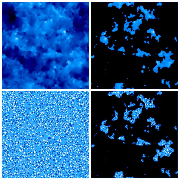
Figure 13: Same as in Fig. 5 but with noise free string induced only temperature fluctuations. Note the interesting structures in the curvature map.

	MAP (dof = 31)			Planck (dof = 47)
	$\chi^{2}$	$\chi^{2}/{\rm dof}$	Prob.	$\chi^{2}$	$\chi^{2}/{\rm dof}$	Prob.
$\beta=1.0$	34.1	1.1	0.32	46.6	0.99	0.49
$\beta=0.0$	109.3	3.52	$3.1\ 10^{-10}$	879.3	18.7	0.0
$\beta=0.7$	120.9	3.9	4.01	217.1	4.6	0.0
$\beta=0.8$	68.2	2.2	$1.3\ 10^{-4}$	180.5	3.84	0.0
$\beta=0.9$	55.8	1.8	$4.0\ 10^{-3}$	101.1	2.15	$7.0\ 10^{-6}$

Table 1: The measured $\chi^{2}$, $\chi^{2}/{\rm dof}$ and significance probability (Prob.) are shown for various values of $\beta$ and for our virtual MAP and Planck experiments, as explained in the text.

In this paper, we have tested a statistic based on local curvature measurements by counting three well defined types of points according to the sign of the eigenvalues of the Hessian of a temperature map. In the first section, we computed the relevant theoretical expectations. We validated them and demonstrated our ability to properly measure them in the next section and eventually introduced this statistic as an accurate non-Gaussianity test (by performing a $\chi^{2}$ like analysis) in the last sections, where we applied it to the case of mixed models with realistic noise levels. Even if our physical simulation might be somewhat simplistic (e.g. no pre-lss string contribution, no foregrounds residuals, etc.), they showed clearly that we are able by using this technique in the Planck context, to distinguish a non-Gaussian background amplitude around 10% in temperature rms (5% in $C_{\ell}$) with a good significance using only 0.3% of the sky and one single channel. Consequently, these results are definitely positive and, as it is, this method seems to be ready to be applied on true data.

Naturally, in practice this test should be used in conjunction with other more standard statistical measurements, like 2-, 3-, 4-,…points correlation functions or their harmonic transform, power spectrum, bispectrum, trispectrum …or even already presented more sophisticated ones like the distribution of wavelet coefficients, etc. This array of methods might actually help in identifying the source of non-gaussianity detected in a realistic context. Indeed, in practical situations, important non-Gaussian effects might be induced by CMB contaminants, in particular galactic foregrounds, residual map stripping or point sources, or any instrumental systematic error.

5.1 Possible advantages

One important advantage of these statistic is its local nature, i.e. the fact that we are only interested by the 8 neighboring pixels. The sphericity of the sky is thus not an issue for this method and so is the pixelisation, provided that the smoothing scale is about 3 times the pixel size (see §3.3).

A second advantage of the method lies in the fact that it is mathematically well-defined and simple since it depends only on one single spectral parameter, $\gamma$ that can be either measured from the fractions themselves or from the $C_{\ell}$ measurement (see §3.3). Thus measurements are well understood and well controlled from a theoretical point of view.

5.2 Outlooks

As we mentioned earlier, by moving to second order derivatives, this work opens the way to many more characterization of random Gaussian field. We expect that an analogous work could be done by considering critical points only, which would lead, e.g. , to a measurement of the Euler characteristic as a function of threshold. However, we expect this restriction to be less efficient in probing non-Gaussianity since it appears that by keeping all types of points we benefit more from the full structure of the probability distribution function. This point will be demonstrated in a future work. In addition, before applying the method to real data, it will also be interesting to compare it’s ability to that of other estimators on the same test protocole, but extended to include other families of models, as e.g. [Lyth & Wands 2001].

References

- [Adler 1981] R. J. Adler, The geometry of random fields, John Wiley & sons, 1981
- [Aghanim & Forni 1999] N. Aghanim & O. Forni, A&A, 347, 409, 1999
- [Aghanim & Forni 2001] N. Aghanim & O. Forni, A&A, 365, 341, 2001
- [Banday et al. 2000] A. Banday, S. Zaroubi & K.M. Górski, ApJ, 533, 575, 2000
- [Bardeeen et al. 1986] J. M. Bardeen,J.R. Bond,N. Kaiser,A.S. Szalay, ApJ, 304, 15, 1986
- [Barreiro et al. 2001] R.B. Barreiro, E. Martínez-Gonz´ alez, & J. L. Sanz 2001, MNRAS, 322, 411
- [Bennett & Bouchet 1990] D.P. Bennett, F. R. Bouchet, Phys. Rev. D, 41, 2408, 1990
- [Bernardeau 1998] F. Bernardeau, A&A, 338, 767, 1998
- [Bond and Efstathiou 1987] J. R. Bond, G. Efstathiou, MNRAS, 226, 655, 1987
- [Bouchet et al. 1988] F. R. Bouchet, D.P. Bennett, A. Stebbins, Nature, 335, 29, 1988
- [Bouchet et al. 2000] F. R. Bouchet, P. Peter, A. Riazuelo, M. Sakellariadou, Phys. Rev. D, D65, 021301, 2001
- [Coles et al. 1989] P. Coles, MNRAS, 238, 319-438, 1989
- [Colombi et al. 2001] S. Colombi, D. Pogosyan, T. Souradeep, Phys. Rev. Let., 85, 5515, 2000
- [Contaldi et al. 2001] C. Contaldi, M. Hindmarsh, J. Magueijo, Phys. Rev. Let., 82, 2034, 1999
- [Ferreira et al. 1998] P.G. Ferreira, J. Magueijo & K.M. Górski, ApJ, 503, 1, 1998
- [Gangui & Martin 2000a] A. Gangui, J. Martin, Phys. Rev. D, D62,103004, 2000
- [Gangui & Martin 2000b] A. Gangui, J. Martin, MNRAS, 313, 323 2000
- [Gott et al. 1990] J. R. Gott et al., ApJ, 352, 1, 1990
- [Lee et al. 2001] A.T. Lee et al. 2001, submitted to ApJ, astro-ph/0104459
- [Luo 1994] X. Luo, Phys. Rev. D, 49, 8, 1994
- [Halverson et al. 2001] N. W. Halverson et al. , submitted to ApJ, astro-ph/0104489
- [Heavens & Sheth 1999] A. F. Heavens, R. Sheth, MNRAS, 310, 1062, 1999
- [Heavens & Gupta 2001] A. F. Heavens, S.J. Gupta, MNRAS, 324, 960, 2001
- [Hinshaw et al. 1995] G. Hinshaw, A.J. Banday,C.L. Bennett, K.M. Gorski, A. Kogut, ApJ, 446L, 67H, 1995
- [Komatsu et al. 2001] E. Komatsu, B.D. Wandelt,D.N. Spergel, A.J. Banday, K.M. Górski 2001, submitted to ApJ,astro-ph/0107605
- [Kunz et al. 2001] M.Kunz et al. , in press, ApJ, 2001
- [Linde & Riotto 1997] A.D. Linde, A. Riotto, Phys. Rev. D, 56, 1842, 1997
- [Lyth & Wands 2001] D. Lyth and D. Wands, Phys.Lett. B524 (2002) 5-14
- [Magueijo 2000] J. Magueijo, ApJ, 528, 57, 2000
- [Netterfield et al. 2001] C.B. Netterfield et al. , astro-ph/0104460, submitted to ApJ, 2001
- [Novikov & Jorgensen 1996] Novikov, D. I. & Jorgensen, H. E. 1996, ApJ, 471, 521
- [Polenta et al. 2002 ] G. Polenta et al. , astro-ph/0201133, submitted to ApJ, 2002
- [Santos et al. 2001] M. G. Santos et al. , astro-ph/0107588
- [Seljak & Zaldarriaga 1996] U. Seljak, M. Zaldarriaga, ApJ, 469,437,1996
- [Smoot et al. 1994] G. Smoot et al. , ApJ, 437, 1, 1994
- [Takada 2001] M. Takada, to appear in ApJ, astro-ph/0101449
- [Vittorio & Juszkiewicz 1987] N. Vittorio & R. Juszkiewicz, ApJ Let., 314, L29, 1987
- [Verde & Heavens 2001] L. Verde, A.F. Heavens, ApJ, 553, 14, 2001