Modern optical astronomy: technology and impact of interferometry

Abstract

The present ‘state of the art’ and the path to future progress in high spatial resolution imaging interferometry is reviewed. The review begins with a treatment of the fundamentals of stellar optical interferometry, the origin, properties, optical effects of turbulence in the Earth’s atmosphere, the passive methods that are applied on a single telescope to overcome atmospheric image degradation such as speckle interferometry, and various other techniques. These topics include differential speckle interferometry, speckle spectroscopy and polarimetry, phase diversity, wavefront shearing interferometry, phase-closure methods, dark speckle imaging, as well as the limitations imposed by the detectors on the performance of speckle imaging. A brief account is given of the technological innovation of adaptive-optics (AO) to compensate such atmospheric effects on the image in real time. A major advancement involves the transition from single-aperture to the dilute-aperture interferometry using multiple telescopes. Therefore, the review deals with recent developments involving ground-based, and space-based optical arrays. Emphasis is placed on the problems specific to delay-lines, beam recombination, polarization, dispersion, fringe-tracking, bootstrapping, coherencing and cophasing, and recovery of the visibility functions. The role of AO in enhancing visibilities is also discussed. The applications of interferometry, such as imaging, astrometry, and nulling are described. The mathematical intricacies of the various ‘post-detection’ image-processing techniques are examined critically. The review concludes with a discussion of the astrophysical importance and the perspectives of interferometry.

CONTENTS

I INTRODUCTION

Optical interferometry provides physicists and astronomers with an exquisite set of probes of the micro and macrocosmos. From the laboratory to the observatory over the past few decades, there has been a surge of activity in developing new tools for ground-based optical astronomy, of which interferometry is one of the most powerful.

An optical interferometer is a device that combines two or more light waves emitted from the same source at the same time to produce interference fringes. The implementation of interferometry in optical astronomy began more than a century ago with the work of Fizeau (1868). Michelson and Pease (1921) measured successfully the angular diameter of ($\alpha$ Ori), using an interferometer based on two flat mirrors, which allowed them to measure the fringe visibility in the interference pattern formed by starlight at the detector plane. However, progress was hindered by the severe image degradation produced by atmospheric turbulence in the optical spectrum. The field remained dormant until the development of intensity interferometry by Hanbury Brown and Twiss (1958), a technique that employs two adjacent sets of mirrors and photoelectric correlation.

Turbulence and the concomitant development of thermal convection in the atmosphere distort the phase and amplitude of an incoming wavefront of starlight. The longer the path, the greater the degradation that the image suffers. Light reaching the entrance pupil of an imaging system is coherent only within patches of diameters of order r_∘ , Fried’s parameter (Fried, 1966). This limited coherence causes blurring of the image, blurring that is modeled by a convolution with the point-spread function (PSF). Both the sharpness of astronomical images and the signal-to-noise (S/N) ratio (hence faintness of the objects that can be studied) depend on angular resolution, the latter because noise comes from as much of the sky as is in the resolution element. Thus reducing the beam width from, say, 1 arcsecond (^′′) to 0.5^′′ reduces sky noise by a factor of 4. Two physical phenomena limit the minimum resolvable angle at optical and infrared (IR) wavelengths - diameter of the collecting area and turbulence in the atmosphere. The crossover between domination by aperture size ($\lambda$/aperture diameter) and domination by atmospheric turbulence (‘seeing’) occurs when the aperture becomes larger than the size of a characteristic turbulent element.

The image of a star obtained through a large telescope looks ‘speckled’ or grainy because different parts of the image are blurred by small areas of turbulence in the earth’s atmosphere. Labeyrie (1970) proposed speckle interferometry (SI), a process that deciphers the diffraction-limited Fourier spectrum and image features of stellar objects by taking a large number of very-short-exposure images of the same field. Computer assistance is then used to reconstruct from these many images a single image that is free of turbulent areas-in essence, an image of the object as it might appear from space.

The success of speckle interferometry in measuring the diameters of stars encouraged astronomers to develop further image-processing techniques. These techniques are, for the most part, post-detection processes. Recent advances in technology have produced the hardware to compensate for wave-front distortion in real time. Adaptive optics (AO; Babcock, 1953; Rousset et al., 1990) is based on this hardware-oriented approach, which sharpens telescope images blurred by the earth’s atmosphere. It employs a combination of deformation of reflecting surfaces (i.e., flexible mirrors) and post-detection image restoration (Roddier, 1999). One of its most successful applications has been in imaging of Neptune’s ring arcs. Adaptive optical imaging systems have been treated in depth by the review of Roggemann et al. (1997), which includes discussion of wavefront compensation devices, wavefront sensors, control systems, performance of AO systems, and representative experimental results. It also deals with the characterization of atmospheric turbulence, the SI technique, and deconvolution techniques for wavefront sensing.

Long-baseline optical interferometry (LBOI) uses two or more optical telescopes to synthesize the angular resolution of a much larger aperture (aperture synthesis) than would be possible with a single mirror. Labeyrie (1975) extended the concept of speckle interferometry to a pair of telescopes in a North-South baseline configuration, and subsequently astronomers have created larger ground-based arrays. A few of these arrays, e.g., the Keck interferometer and the Very Large Telescope Interferometer (VLTI), employ large telescopes fitted with AO systems. The combination of long-baseline interferometry, mimicking a wide aperture, and AO techniques to improve the images offers the best of both approaches and shows great promise for applications such as the search for extra-solar planets. At this point it seems clear that interferometry and AO are complementary, and neither can reach its full potential without the other.

The present review addresses the aims, methods, scientific achievements, and future prospects of long-baseline interferometry (LBI) at optical and infrared wavelengths, carried out with two or more apertures separated by more than their own sizes. In order to embark on such a subject, we first review the basic principles of interferometry and its applications, the theoretical aspects of SI as a statistical analysis of a speckle pattern, and the limitations imposed by the atmosphere and the detectors on the performance of single-aperture diffraction-limited imaging. Other related concerns, such as the relationship between image-plane techniques and pupil-plane interferometry, phase-closure methods, and dark speckle imaging, will also be treated. Adaptive optics as a pre-detection compensation technique is described in brief, as are the strengths and weaknesses of pre and post detection.

The final part of this review deals with the applications of multiple-telescope interferometry to imaging, astrometry, and nulling. These applications entail specific problems having to do with delaylines, beam recombination, polarization, dispersion, fringe tracking, and the recovery of visibility functions. Various image restoration techniques are discussed as well, with emphasis on the deconvolution methods used in aperture-synthesis mapping.

II BASIC PRINCIPLES

Astronomical sources emit incoherent light consisting of the random superposition of numerous successive short-lived waves sent out from many elementary emitters, and therefore, the optical coherence is related to the various forms of correlations of the random process. For a monochromatic wave field, the amplitude of vibration at any point is constant and the phase varies linearly with time. Conversely, the amplitude and phase in the case of quasi-monochromatic wave field, undergo irregular fluctuations (Born and Wolf, 1984). The rapidity of fluctuations depends on the light crossing time of the emitting region. Interferometers based on (i) wavefront division (Young’s experiment that is sensitive to the size and bandwidth of the source), (ii) amplitude division (Michelson’s interferometer) are generally used to measure spatial coherence and temporal coherence, respectively. In what follows, some of the fundamental mathematical steps pertinent to the interferometry are illustrated.

A Mathematical framework

A monochromatic plane wave, $V{\bf(r},t)$ at a point, ${\bf r}$, is expressed as,

$$V{\bf(r},t)=\Re\left\{{\it a}({\bf r})e^{-i[2\pi\nu_{\circ}t-\psi_{j}({\bf r})]}\right\}.$$ (1)

Here the symbol $\Re$ is the ‘real part of’, ${\bf r}$ the position vector of a point $(x,y,z)$, ${\it a}({\bf r})$ is the amplitude of the wave, $t$ the time, $\nu_{\circ}$ the frequency of the wave, $\psi_{j}({\bf r})$ the phase functions that are of the form ${\bf k\cdot r}-\delta_{j}$, in which ${\bf k}$ is the propagation vector, and $\delta_{j}$ the phase constants which specify the state of polarization, Denoting the complex vector function of position by $\Psi({\bf r})={\it a}({\bf r})e^{i\psi_{j}({\bf r})}$, the complex representation of the analytic signal, ${\cal U}{\bf(r},t)$, associated with $V{\bf(r},t)$ becomes,

$${\cal U}{\bf(r},t) = {\it a}({\bf r})e^{-i[2\pi\nu_{\circ}t-\psi_{j}({\bf r})]}$$ (3)

$$=\Psi({\bf r})e^{-i2\pi\nu_{\circ}t}.$$

This complex representation is preferred for linear time invariant systems, because the eigenfunctions of such systems are of the form $e^{-i\omega_{\circ}t}$, where $\omega_{\circ}=2\pi\nu_{\circ}$ is the angular frequency. From equations (1) and (2), the relationship translates into,

$$V{\bf(r},t) = \Re\left\{\Psi({\bf r})e^{-i\omega_{\circ}t}\right\}$$ (5)

$$=\frac{1}{2}\left[\Psi({\bf r})e^{-i\omega_{\circ}t}+\Psi^{\ast}({\bf r})e^{i\omega_{\circ}t}\right],$$

The intensity of light is defined as the time average of the amount of energy, therefore, taking the latter over an interval much greater than the period, ${\tt T_{\circ}}=2\pi/\omega_{\circ}$, the intensity ${\cal I}$ at the same point is calculated as,

$${\cal I}\propto<V^{2}>=\frac{1}{2}\Psi\Psi^{\ast},$$ (6)

where $<\ >$ stands for the ensemble average of the quantity within the bracket and $\Psi^{\ast}$ represents for the complex conjugate of $\Psi$.

Since the complex amplitude is a constant phasor in the monochromatic case, the Fourier transform (FT) of the complex representation of the signal, ${\cal U}{\bf(r},t)$, is given by,

$$\widehat{\cal U}{\bf(r},\nu)={\it a}({\bf r})e^{i\psi}\delta(\nu-\nu_{\circ}).$$ (7)

It is equal to twice the positive part of the instantaneous spectrum, $\widehat{V}{\bf(r},\nu)$. In the polychromatic case, the complex amplitude becomes,

$${\cal U}{\bf(r},t)=2\int_{0}^{\infty}\widehat{V}{\bf(r},\nu)e^{-i2\pi\nu t}d\nu.$$ (8)

The disturbance produced by a real physical source is calculated by the integration of the monochromatic signals over an optical band pass. In the case of quasi-monochromatic approximation (if the width of the spectrum, $\Delta\nu\ll\nu_{\circ}$), the expression modifies as,

$${\cal U}{\bf(r},t)=|\Psi({\bf r},t)|e^{i[\psi(t)-2\pi\nu_{\circ}t]},$$ (9)

where the field is characterized by the complex amplitude, $\Psi{(\bf r},t)$, i.e.,

$$\Psi{(\bf r},t)=|\Psi({\bf r},t)|e^{i\psi(t)}.$$ (10)

This phasor is time dependent, although it varies slowly with respect to $e^{-i2\pi\nu_{\circ}t}$.

The complex amplitude, $\Psi({\kern-0.24994pt\hbox{$\alpha$}\kern-6.39702pt\kern 0.50003pt\hbox{$\alpha$}\kern-6.39702pt\kern-0.24994pt\raise 0.43304pt\hbox{$\alpha$}})$ diffracted at angle $\alpha$$\alpha$$\alpha$ in the telescope focal-plane is given by,

$$\Psi({\kern-0.24994pt\hbox{$\alpha$}\kern-6.39702pt\kern 0.50003pt\hbox{$\alpha$}\kern-6.39702pt\kern-0.24994pt\raise 0.43304pt\hbox{$\alpha$}})\propto\int{\cal P}_{\circ}({\bf x})\Psi_{\circ}({\bf x})e^{-i2\pi{\kern-0.17496pt\hbox{$\alpha$}\kern-4.4779pt\kern 0.35002pt\hbox{$\alpha$}\kern-4.4779pt\kern-0.17496pt\raise 0.30313pt\hbox{$\alpha$}}.{\bf x}/\lambda}d{\bf x},$$ (11)

where ${\kern-0.24994pt\hbox{$\alpha$}\kern-6.39702pt\kern 0.50003pt\hbox{$\alpha$}\kern-6.39702pt\kern-0.24994pt\raise 0.43304pt\hbox{$\alpha$}}=({\bf x}/{f})$ is a two-dimensional (2-d) space vector, ${f}$ the focal length, $\Psi_{\circ}({\bf x})$ the complex amplitude at the telescope aperture, and ${\cal P}_{\circ}({\bf x})$ the pupil transmission function of the telescope aperture. For an ideal telescope, we have ${\cal P}_{\circ}({\bf x})=1$ inside the aperture and ${\cal P}_{\circ}({\bf x})=0$ outside the aperture. In the space-invariant case,

$$\Psi({\kern-0.24994pt\hbox{$\alpha$}\kern-6.39702pt\kern 0.50003pt\hbox{$\alpha$}\kern-6.39702pt\kern-0.24994pt\raise 0.43304pt\hbox{$\alpha$}}) \propto \int{\cal P}({\bf u})\Psi({\bf u})e^{-i2\pi{\kern-0.17496pt\hbox{$\alpha$}\kern-4.4779pt\kern 0.35002pt\hbox{$\alpha$}\kern-4.4779pt\kern-0.17496pt\raise 0.30313pt\hbox{$\alpha$}}{\bf u}}d{\bf u},$$ (13)

$$={\cal F}[\Psi({\bf u})\cdot{\cal P}({\bf u})],$$

where ${\cal F}$ represents for the complex FT and the dimensionless variable ${\bf u}$ is equal to ${\bf x}/\lambda$ and hence, $\Psi({\bf u})$ can be replaced by $\Psi_{\circ}(\lambda{\bf u})$ and so with ${\cal P}({\bf u})$ by ${\cal P}_{\circ}(\lambda{\bf u})$. The irradiance diffracted in the direction $\alpha$$\alpha$$\alpha$ is the PSF of the telescope and the atmosphere and its FT, $\widehat{\cal S}({\bf f})$ is the optical transfer function (OTF):

$$\widehat{\cal S}({\bf f})=\int{\cal S}({\kern-0.24994pt\hbox{$\alpha$}\kern-6.39702pt\kern 0.50003pt\hbox{$\alpha$}\kern-6.39702pt\kern-0.24994pt\raise 0.43304pt\hbox{$\alpha$}})e^{[-2i\pi{\kern-0.17496pt\hbox{$\alpha$}\kern-4.4779pt\kern 0.35002pt\hbox{$\alpha$}\kern-4.4779pt\kern-0.17496pt\raise 0.30313pt\hbox{$\alpha$}}.{\bf f}]}d{\kern-0.24994pt\hbox{$\alpha$}\kern-6.39702pt\kern 0.50003pt\hbox{$\alpha$}\kern-6.39702pt\kern-0.24994pt\raise 0.43304pt\hbox{$\alpha$}},$$ (14)

where ${\bf f}$ is the spatial frequency expressed in radian^-1, and $|\widehat{\cal S}({\bf f})|$ the modulation transfer function (MTF).

1 Convolution

The convolution of two functions simulates phenomena such as a blurring of a photograph that may be caused by various reasons, e.g., (a) poor focus, (b) motion of a photographer during the exposure. In such a blurred picture each point of object is replaced by a spread function. For the 2-d incoherent source, the complex amplitude in the image-plane is the convolution of complex amplitude of the pupil plane and the pupil transmission function.

$${\cal S}({\kern-0.24994pt\hbox{$\alpha$}\kern-6.39702pt\kern 0.50003pt\hbox{$\alpha$}\kern-6.39702pt\kern-0.24994pt\raise 0.43304pt\hbox{$\alpha$}})={\cal P}({\kern-0.24994pt\hbox{$\alpha$}\kern-6.39702pt\kern 0.50003pt\hbox{$\alpha$}\kern-6.39702pt\kern-0.24994pt\raise 0.43304pt\hbox{$\alpha$}})\star\Psi({\kern-0.24994pt\hbox{$\alpha$}\kern-6.39702pt\kern 0.50003pt\hbox{$\alpha$}\kern-6.39702pt\kern-0.24994pt\raise 0.43304pt\hbox{$\alpha$}}).$$ (15)

In the Fourier plane, the effect of the convolution becomes a multiplication, point by point of the OTF of the pupil, ${\cal P}({\bf u})$, with the transform of the object $\Psi({\bf u})$. i.e.,

$$\widehat{\cal S}({\bf f})={\cal P}({\bf u})\cdot\Psi({\bf u}).$$ (16)

The illumination at the focal-plane of the telescope observed as a function of image-plane is,

$${\cal S}({\kern-0.24994pt\hbox{$\alpha$}\kern-6.39702pt\kern 0.50003pt\hbox{$\alpha$}\kern-6.39702pt\kern-0.24994pt\raise 0.43304pt\hbox{$\alpha$}}) = <\Psi({\kern-0.24994pt\hbox{$\alpha$}\kern-6.39702pt\kern 0.50003pt\hbox{$\alpha$}\kern-6.39702pt\kern-0.24994pt\raise 0.43304pt\hbox{$\alpha$}},t)\Psi^{\ast}({\kern-0.24994pt\hbox{$\alpha$}\kern-6.39702pt\kern 0.50003pt\hbox{$\alpha$}\kern-6.39702pt\kern-0.24994pt\raise 0.43304pt\hbox{$\alpha$}},t)>,$$ (18)

$$\propto|{\cal F}[\Psi({\bf u})\cdot\Psi^{\ast}({\bf u})]|^{2}.$$

The autocorrelation of this function, ${\cal S}({\kern-0.24994pt\hbox{$\alpha$}\kern-6.39702pt\kern 0.50003pt\hbox{$\alpha$}\kern-6.39702pt\kern-0.24994pt\raise 0.43304pt\hbox{$\alpha$}})$, is expressed as,

$${\cal F}[{\cal S}({\kern-0.24994pt\hbox{$\alpha$}\kern-6.39702pt\kern 0.50003pt\hbox{$\alpha$}\kern-6.39702pt\kern-0.24994pt\raise 0.43304pt\hbox{$\alpha$}})\otimes{\cal S}({\kern-0.24994pt\hbox{$\alpha$}\kern-6.39702pt\kern 0.50003pt\hbox{$\alpha$}\kern-6.39702pt\kern-0.24994pt\raise 0.43304pt\hbox{$\alpha$}})]=\widehat{\cal S}({\bf f})\widehat{\cal S}^{\ast}({\bf f})=|\widehat{\cal S}{\bf(f)}|^{2},$$ (19)

where $\otimes$ stands for correlation.

2 Resolution

In an ideal condition, the resolution that can be achieved in an imaging experiment, ${\cal R}$, is limited only by the imperfections in the optical system and according to Strehl’s criterion, the resolving power, ${\cal R}$, of any telescope of diameter $D$ is given by the integral of its transfer function,

$${\cal R}=\int\widehat{\cal S}({\bf u})d{\bf u}.$$ (20)

Therefore, ${\cal R}={\cal S}({\bf 0})$. The Strehl ratio ${\cal S}_{r}$ is defined as the ratio of the intensity at the centroid of the observed PSF, ${\cal S}({\bf 0)}$, to the intensity of the peak of the diffraction-limited image or ‘Airy spike’, ${\cal S}({\bf 0})_{{\cal A}s}$, i.e.,

$${\cal S}_{r} = \frac{{\cal S}({\bf 0})}{{\cal S}({\bf 0})_{{\cal A}s}}$$ (22)

$$\approx e^{-k^{2}\sigma^{2}_{OPD}},$$

where $k=2\pi/\lambda$ is the wave number and $\sigma_{OPD}$ the rms optical path difference (OPD) error. Typical ground-based observations with large telescopes in the visible wavelength range are made with a Strehl ratio $\leq 0.01$ (Babcock, 1990), while a diffraction-limited telescope would, by definition, have a Strehl ratio of 1.

B Principles of interference and its applications

When two light beams from a single source are superposed, the intensity at the place of superposition varies from point to point between maxima, which exceed the sum of the intensities in the beams, and minima, which may be zero. This sum or difference is known as interference; the correlated fluctuation can be partially or completely coherent (Born and Wolf, 1984).

Let the two monochromatic waves $V_{1}({\bf r},t)$ and $V_{2}({\bf r},t)$ be superposed at the recombination point. The correlator sums the instantaneous amplitudes of the fields. The total field at the output is,

$$V = V_{1}+V_{2},$$ (23)

$$V^{2} = V^{2}_{1}+V^{2}_{2}+2V_{1}\cdot V_{2}.$$ (24)

Then if $\Psi_{1}$ and $\Psi_{2}$ are the complex amplitudes of the two waves, with the corresponding phases $\psi_{1}$ and $\psi_{2}$, these two waves are propagating in $z$ direction and linearly polarized with electric field vector in $x$ direction. (A general radiation field is generally described by four Stokes parameters $I$, $Q$, $U$, and $V$, that specify intensity, the degree of polarization, the plane of polarization and the ellipticity of the radiation at each point and in any given direction). Therefore, the total intensity, (see equation 4), at the same point can be determined as,

$${\cal I} = {\cal I}_{1}+{\cal I}_{2}+{\cal J}_{12}$$ (27)

$$={\cal I}_{1}+{\cal I}_{2}+\frac{1}{2}\left(\Psi_{1}\Psi_{2}^{\ast}+\Psi_{1}^{\ast}\Psi_{2}\right)$$

$$={\cal I}_{1}+{\cal I}_{2}+2\sqrt{{\cal I}_{1}{\cal I}_{2}}\ \cos\delta,$$

where ${\cal I}_{1}=<V_{1}^{2}>$, and ${\cal I}_{2}=<V_{2}^{2}>$, are the intensities of the two terms, and ${\cal J}_{12}=2<V_{1}\cdot V_{2}>=2\sqrt{{\cal I}_{1}{\cal I}_{2}}$, is the interference term that depends on the amplitude components, as well as on the phase-difference between the two waves, $\delta=2\pi\Delta\varphi/\lambda_{\circ}$, ($\Delta\varphi$, is the OPD between the two waves from the common source to the intersecting point and $\lambda_{\circ}$ is the wavelength in vacuum). In general, two light beams are not correlated but the correlation term, $\Psi_{1}\Psi_{2}^{\ast}$, takes on significant values for a short period of time and $<\Psi_{1}\Psi_{2}^{\ast}>$ = 0. Time variations of $\Psi({\bf r})$ are statistical in nature (Mendel and Wolf, 1995). Hence, one seeks a statistical description of the field (correlations) as the field is due to a partially coherent source. Depending upon the correlations between the phasor amplitudes at different object points, one would expect a definite correlation between the two points of the field emitted by the object. The maximum and minimum intensity occur, when $|\delta|=0,2\pi,4\pi$ and $|\delta|=\pi,3\pi,5\pi$, respectively. If ${\cal I}_{1}={\cal I}_{2}={\cal I}$, the intensity varies between 4${\cal I}$, and 0.

In the case of quasi-monochromatic wave, the analytical signal, ${\cal U}(t)$, obtained at the observation point is expressed as,

$${\cal U}(t)=K_{1}{\cal U}(r_{1},t-\tau_{1})+K_{2}{\cal U}(r_{2},t-\tau_{2}),$$ (28)

where $K_{j}$’s are constants, $r_{j}$’s the positions of two pinholes in the wave field, j = 1, 2, ${\it s}_{j}$’s the distances of a meeting point of the two beams from the two pinholes, $\tau_{j}={\it s}_{j}/c$, the time needed to travel from the respective pinholes to the meeting point, and $c$ the velocity of light.

If the pinholes are small and the diffracted fields are considered to be uniform, the value $K_{j}$ of the constants, $|K_{j}|$ turns out to be, $K_{1}^{\ast}K_{2}=K_{1}K^{\ast}_{2}=K_{1}K_{2}$ and noting, ${\cal I}_{j}=|K_{j}|^{2}<|{\cal U}(r_{j},t-\tau_{j})|^{2}>$, and therefore, the intensity at the output is found to be,

$${\cal I}={\cal I}_{1}+{\cal I}_{2}+2K_{1}K_{2}\Re\left[{\bf\Gamma}_{12}\left(\frac{s_{2}-s_{1}}{c}\right)\right].$$ (29)

The Van Cittert-Zernike theorem states that the modulus of the complex degree of coherence (describes the correlation of vibrations at a fixed point and a variable point) in a plane illuminated by a incoherent quasi-monochromatic source is equal to the modulus of the normalized spatial FT of its brightness distribution (Born and Wolf, 1984, Mendel and Wolf, 1995). The observed image is the FT of the mutual coherence function or the correlation function. The complex degree of (mutual) coherence, ${\kern-0.24994pt\hbox{$\gamma$}\kern-5.1773pt\kern 0.50003pt\hbox{$\gamma$}\kern-5.1773pt\kern-0.24994pt\raise 0.43304pt\hbox{$\gamma$}}_{12}(\tau)$, of the observed source is defined as,

$${\kern-0.24994pt\hbox{$\gamma$}\kern-5.1773pt\kern 0.50003pt\hbox{$\gamma$}\kern-5.1773pt\kern-0.24994pt\raise 0.43304pt\hbox{$\gamma$}}_{12}(\tau)=\frac{{\bf\Gamma}_{12}(\tau)}{\sqrt{{\bf\Gamma}_{11}(0){\bf\Gamma}_{22}(0)}}=\frac{{\bf\Gamma}_{12}(\tau)}{\sqrt{{\cal I}_{1}{\cal I}_{2}}},$$ (30)

where ${\cal I}_{1}=K_{1}^{2}{\bf\Gamma}_{11}(0)$ and ${\cal I}_{2}=K_{2}^{2}{\bf\Gamma}_{22}(0)$. The function, ${\bf\Gamma}_{ij}(\tau)=<{\cal U}(r_{i},t+\tau){\cal U}^{\ast}(r_{j},t)>$, is measured at two points. At a point where both the points coincide, the self coherence, ${\bf\Gamma}_{11}(\tau)=<{\cal U}(r_{1},t+\tau){\cal U}^{\ast}(r_{1},t)>$, reduces to ordinary intensity. When $\tau=0$, ${\bf\Gamma}_{11}(0)={\cal I}_{1};{\bf\Gamma}_{22}(0)={\cal I}_{2}$. The ensemble average can be replaced by a time average due to the assumed ergodicity (a random process that is strictly stationary) of the fields. If both the fields are directed on a quadratic detector, it yields the desired cross-term (time average due to the finite time response). The measured intensity at the detector would be,

$${\cal I}={\cal I}_{1}+{\cal I}_{2}+2\sqrt{{\cal I}_{1}.{\cal I}_{2}}\Re\left[{\kern-0.24994pt\hbox{$\gamma$}\kern-5.1773pt\kern 0.50003pt\hbox{$\gamma$}\kern-5.1773pt\kern-0.24994pt\raise 0.43304pt\hbox{$\gamma$}}_{12}\left(\frac{s_{2}-s_{1}}{c}\right)\right].$$ (31)

In order to keep the time correlation close to unity, the delay, $\tau$, must be limited to a small fraction of the temporal width or coherence time, $\tau_{c}=1/\Delta\nu$; here $\Delta\nu$, is the spectral width. The relative coherence of the two beams diminishes with the increase of path length difference, culminating in a drop in the visibility (a dimensionless number between zero and one that indicates the extent to which a source is resolved on the baseline being used) of the fringes. For $\tau\ll\tau_{c}$, the function, ${\kern-0.24994pt\hbox{$\gamma$}\kern-5.1773pt\kern 0.50003pt\hbox{$\gamma$}\kern-5.1773pt\kern-0.24994pt\raise 0.43304pt\hbox{$\gamma$}}_{12}(\tau)$, can be approximated to, ${\kern-0.24994pt\hbox{$\gamma$}\kern-5.1773pt\kern 0.50003pt\hbox{$\gamma$}\kern-5.1773pt\kern-0.24994pt\raise 0.43304pt\hbox{$\gamma$}}_{12}(0)e^{-2\pi i\nu_{\circ}\tau}$. The exponential term is nearly constant and ${\kern-0.24994pt\hbox{$\gamma$}\kern-5.1773pt\kern 0.50003pt\hbox{$\gamma$}\kern-5.1773pt\kern-0.24994pt\raise 0.43304pt\hbox{$\gamma$}}_{12}(0)$, measures the spatial coherence. Let $\psi_{12}$, be the argument of ${\kern-0.24994pt\hbox{$\gamma$}\kern-5.1773pt\kern 0.50003pt\hbox{$\gamma$}\kern-5.1773pt\kern-0.24994pt\raise 0.43304pt\hbox{$\gamma$}}_{12}(\tau)$, then,

$${\cal I}={\cal I}_{1}+{\cal I}_{2}+2\sqrt{{\cal I}_{1},{\cal I}_{2}}\Re\left[|{\kern-0.24994pt\hbox{$\gamma$}\kern-5.1773pt\kern 0.50003pt\hbox{$\gamma$}\kern-5.1773pt\kern-0.24994pt\raise 0.43304pt\hbox{$\gamma$}}_{12}(0)|e^{i(\psi_{12}-2\pi\nu_{\circ}\tau)}\right].$$ (32)

The measured intensity at a distance $x$ from the origin (point at zero OPD) on a screen at a distance, $z$, from the apertures is

$${\cal I}(x) = {\cal I}_{1}+{\cal I}_{2}+2\sqrt{{\cal I}_{1},{\cal I}_{2}}|{\kern-0.24994pt\hbox{$\gamma$}\kern-5.1773pt\kern 0.50003pt\hbox{$\gamma$}\kern-5.1773pt\kern-0.24994pt\raise 0.43304pt\hbox{$\gamma$}}_{12}(0)|$$ (34)

$$\cos\left\{\frac{2\pi d(x)}{\lambda}-\psi_{12}\right\},$$

where $d(x)=bx/z$, is the OPD corresponding to $x$, and $b$ the distance between the two apertures.

The modulus of the fringe visibility is estimated as the ratio of high frequency to low frequency energy in the average spectral density; the visibility of fringes, ${\cal V}$, is estimated as,

$${\cal V}=\frac{{\cal I}_{max}-{\cal I}_{min}}{{\cal I}_{max}+{\cal I}_{min}}=|{\kern-0.24994pt\hbox{$\gamma$}\kern-5.1773pt\kern 0.50003pt\hbox{$\gamma$}\kern-5.1773pt\kern-0.24994pt\raise 0.43304pt\hbox{$\gamma$}}_{12}(0)|\frac{2\sqrt{{\cal I}_{1}{\cal I}_{2}}}{{\cal I}_{1}+{\cal I}_{2}}.$$ (35)

1 Fizeau interferometer

Fizeau (1868) suggested that installing a screen with two holes in front of a telescope would allow measurements of stellar diameters with diffraction-limited resolution. In this set up, the beams are diffracted by the sub-apertures and the telescope acts as both collector and correlator. Therefore, temporal coherence is automatically obtained due to the built-in zero OPD. The spatial modulation frequency, as well as the required sampling of the image change with the separation of sub-apertures. The maximum resolution in this case depends on the separation between the sub-apertures; the maximum spacings that can be explored are limited by the physical diameter of the telescope. The number of stellar sources for measuring diameters is also limited. One of the first significant results was the measurement of the diameter of the satellites of Jupiter with a Fizeau interferometer on the 40-inch Yerkes refractor by Michelson (1891). With the 100-inch telescope on Mt. Wilson Anderson (1920) determined the angular separation ($\rho$) of spectroscopic binary star Capella.

2 Michelson interferometer

Results from the classical Michelson interferometer were used to formulate special relativity. They are also being used in gravity-wave detection. Gravitational radiation produced by coalescing binaries, or exploding stars, for example, changes the metric of spacetime. This effect causes a differential change of the path length of the arms of the interferometer, thereby introducing a phase-shift. Today, there are several ground-based long baseline laser-interferometric detectors based on this principle under construction, and within the next several years these detectors should be in operation (Robertson, 2000). The proposed laser interferometer space antenna, consisting of three satellites in formation about 50 million kilometers (km) above the Earth in a heliocentric orbit, may detect gravitational waves by measuring fluctuations in the distances between test masses carried by the satellites.

The essence of the Michelson’s stellar interferometer is to determine the covariance $<\Psi_{1}\Psi_{2}>$ of the complex amplitudes $\Psi_{1},\Psi_{2}$, at two different points of the wavefronts. This interferometer was equipped with four flat mirrors that fold the beams by installing a 7-meter (m) steel beam on top of the Mt. Wilson 100-inch telescope. Michelson and Pease (1921) resolved the supergiant $\alpha$ Ori and a few other stars. In this case, the spatial modulation frequency in the focal-plane is independent of the distance between the collectors. In the Fizeau mode, the ratio of aperture diameter/separation is constant from light collection to recombination in the image-plane (homothetic pupil). In the Michelson mode, this ratio is not constant since the collimated beams have the same diameter from the output of the telescope to the recombination lens. The distance between pupils is equal to the baseline at the collection mirrors (the resolution is limited by the baseline) and to a much smaller value just before the recombination lens. The disadvantage of the Michelson mode is a very narrow field of view compared to the Fizeau mode. Unfortunately the project was abandoned due to various difficulties, including (i) effect of atmospheric turbulence, (ii) variations of refractive index above the small sub-aperture, (iii) inadequate separation of outer mirrors, and (iv) mechanical instability.

3 Intensity interferometer

Intensity interferometry considers the quantum theory of photon detection and correlation. It computes the fluctuations of the intensities ${\cal I}_{1},{\cal I}_{2}$, at two different points of the wavefronts. The fluctuations of the electrical signals from the two detectors are compared by a multiplier. The current output of each photoelectric detector is proportional to the instantaneous intensity ${\cal I}$ of the incident light, which is the squared modulus of the amplitude $\Psi$. The fluctuation of the current output is proportional to $\Delta{\cal I}=|\Psi|^{2}-<|\Psi|^{2}>$. The covariance of the fluctuations, according to Goodman (1985), can be expressed as,

$$<\Delta{\cal I}_{1}\Delta{\cal I}_{2}>=<|\Psi_{1}\Psi_{2}^{\ast}|^{2}>.$$ (36)

This expression indicates that the covariance of the intensity fluctuations is the squared modulus of the covariance of the complex amplitude.

Having succeeded in completing the intensity interferometer at radio wavelengths (Hanbury Brown et al. 1952), Hanbury Brown and Twiss (1958) demonstrated its potential at optical wavelengths by measuring the angular diameter of Sirius. Subsequent development with a pair of 6.5 m light collector on a circular railway track spanning 188 m, provided the measurements of 32 southern binary stars (Hanbury Brown, 1974) with angular resolution limit of 0.5 milli-arcseconds (mas). In this arrangement, starlight collected by two concave mirrors is focused on to two photoelectric cells and the correlation of fluctuations in the photocurrents is measured as a function of mirror separation. The advantages of such a system over Michelson’s interferometer are that it does not require high mechanical stability and remains unaffected by seeing. Another noted advantage is that the alignment tolerances are extremely relaxed since the pathlengths need to be maintained to a fraction of $c/{\it b}_{e}$, where ${\it b}_{e}$ is the electrical bandwidth of the post-detection electronics. The significant effect comes from scintillation induced by the atmosphere. The sensitivity of this interferometer was found to be very low; it was limited by the narrow band-width filters that are used to increase the speckle life time. The correlated fluctuations can be obtained if the detectors are spaced by less than a speckle width. Theoretical calculations (Roddier, 1988) show that the limiting visual magnitude (mag), $m_{v}$ that can be observed with such a system is of the order of 2 (the faintest stars visible in the naked eye are 6th magnitude. The magnitude scale is defined as $m_{1}-m_{2}$ = -2.5 log $F_{1}/F_{2}$, where $m_{1}$ and $m_{2}$ are the apparent magnitudes of two objects of fluxes $F_{1}$ and $F_{2}$, respectively).

III ATMOSPHERIC TURBULENCE

The density inhomogeneities appear to be created and maintained by the parameters, viz., thermal gradients, humidity fluctuations, and wind shears, which produce atmospheric turbulence and therefore refractive index inhomogeneities. The gradients caused by these environmental parameters warp the wavefront incident on the telescope pupil. The image quality is directly related to the statistics of the perturbations of the incoming wavefront. The theory of seeing combines the theory of atmospheric turbulence with the theory of optical physics to predict the modifications to the diffraction-limited image that the refractive index gradients produce (Young, 1974, Roddier, 1981, Coulman, 1985). Atmospheric turbulence has a significant effect on the propagation of radio-waves, sound-waves and on the flight of aircraft as well. This section is devoted to the descriptions of the atmospheric turbulence theory, metrology of seeing and its impact on stellar images.

A Formation of eddies

The random fluctuations in the atmospheric motions occur predominantly due to (i) the friction encountered by the air flow at the Earth’s surface and consequent formation of a wind-velocity profile with large vertical gradients, (ii) differential heating of different portions of the Earth’s surface and the concomitant development of thermal convection, (iii) processes associated with formation of clouds involving release of heat of condensation and crystallization, and subsequent changes in the nature of temperature and wind velocity fields, (iv) convergence and interaction of air-masses with various atmospheric fronts, and (v) obstruction of air-flows by mountain barriers that generate wave-like disturbances and rotor motions on their lee-side.

The atmosphere is difficult to study due to the high Reynolds number ($Re\sim 10^{6}$), a dimensionless quantity, that characterizes the turbulence. When the average velocity, $v_{a}$, of a viscous fluid of characteristic size, $l$, is gradually increased, two distinct states of fluid motion are observed (Tatarski, 1967, Ishimaru, 1978), viz., (i) laminar (regular and smooth in space and time), at very low $v_{a}$, and (ii) unstable and random fluid motion at $v_{a}$ greater than some critical value. The Reynolds number, obtained by equating the inertial and viscous forces, is given by,

$$Re=v_{a}l/\nu_{v}.$$ (37)

where $Re$ is a function of the flow geometry, $v_{a},l$, and kinematic viscosity of the fluid, $\nu_{v}$. When $Re$ exceeds critical value in a pipe (depending on its geometry), a transition of the flow from laminar to turbulent or chaotic occurs. Between these two extreme conditions, the flow passes through a series of unstable states. High $Re$ turbulence is chaotic in both space and time and exhibits considerable spatial structure.

The velocity fluctuations occur on a wide range of space and time scales. According to the atmospheric turbulence model (Taylor, 1921, Kolmogorov, 1941b, 1941c), the energy enters the flow at low frequencies at scale length, $L_{\circ}$ and spatial frequency, $k_{L_{\circ}}=2\pi/L_{\circ}$, as a direct result of the non-linearity of the Navier-Stokes equation governing fluid motion. The large-scale fluctuations, referred to as large eddies, have a size of the geometrically imposed outer scale length $L_{\circ}$. These eddies are not universal with respect to flow geometry; they vary according to the local conditions. Conan et al. (2000) derived a mean value $L_{\circ}=$ 24 m for a von Kármán spectrum from the data obtained at Cerro Paranal, Chile.

The energy is transported to smaller and smaller loss-less eddies until at a small enough Reynolds number, the kinetic energy of the flow is converted into heat by viscous dissipation resulting in a rapid drop in power spectral density, $\Phi_{n}({\bf k})$ for $k>k_{\circ}$, where $k_{\circ}$ is critical wave number. These changes are characterized by the inner scale length, $l_{\circ}$, and spatial frequency, $k_{l_{\circ}}=2\pi/l_{\circ}$, where $l_{\circ}$ varies from a few millimeter near the ground to a centimeter (cm) high in the atmosphere. The small-scale fluctuations with sizes $l_{\circ}<r<L_{\circ}$, known as the inertial subrange, where $r$ is the magnitude of ${\bf r}$, have universal statistics (scale-invariant behavior) independent of the flow geometry. The value of inertial subrange would be different at various locations on the site. The statistical distribution of the size and number of these eddies is characterized by $\Phi_{n}({\bf k})$, of $n_{1}({\bf r},t)$, where $n_{1}({\bf r},t)$ is a randomly fluctuating term, and $t$ the time. The dependence of the refractive index of air $n({\bf r},t)$, upon pressure, $P$ (millibar) and temperature, $T$ (Kelvin), at optical wavelengths is given by $n_{1}\cong n-1=77.6~{}\times~{}10^{-6}P/T$ (Ishimaru, 1978).

B Kolmogorov turbulence model

The optically important property of the Kolmogorov law is that the refractive index fluctuations are largest for the largest turbulent elements up to the outer scale of the turbulence. At sizes below the outer scale, the one-dimensional (1-d) power spectrum of the refractive index fluctuations falls off with -(5/3) power of frequency and is independent of the direction along the fluctuations are measured, i.e., the small-scale fluctuations are isotropic (Young, 1974). The three-dimensional (3-d) power spectrum, $\Phi_{n}$, for the wave number, $k>k_{\circ}$, in the case of inertial subrange, can be equated as,

$$\Phi_{n}({\bf k})=0.033{\cal C}_{n}^{2}k^{-11/3},$$ (38)

where ${\cal C}_{n}^{2}$ is known as the structure constant of the refractive index fluctuations.

This Kolmogorov-Obukhov model of turbulence, describing the power-law spectrum for the inertial intervals of wave numbers, is valid within the inertial subrange and is widely used for astronomical purposes (Tatarski 1993). The refractive index structure function, ${\cal D}_{n}({\bf r})$, is defined as,

$${\cal D}_{n}({\bf r})=<|n\left({\kern-0.24994pt\hbox{$\rho$}\kern-5.17015pt\kern 0.50003pt\hbox{$\rho$}\kern-5.17015pt\kern-0.24994pt\raise 0.43304pt\hbox{$\rho$}}+{\bf r}\right)-n\left({\kern-0.24994pt\hbox{$\rho$}\kern-5.17015pt\kern 0.50003pt\hbox{$\rho$}\kern-5.17015pt\kern-0.24994pt\raise 0.43304pt\hbox{$\rho$}}\right)|^{2}>,$$ (39)

which expresses its variance at two points $r_{1}$, and $r_{2}$.

The structure functions are related to the covariance function, ${\cal B}_{n}({\bf r})$, through

$${\cal D}_{n}({\bf r)}=2[{\cal B}_{n}({\bf 0})-{\cal B}_{n}({\bf r})],$$ (40)

where ${\cal B}_{n}({\bf r})=<n\left({\kern-0.24994pt\hbox{$\rho$}\kern-5.17015pt\kern 0.50003pt\hbox{$\rho$}\kern-5.17015pt\kern-0.24994pt\raise 0.43304pt\hbox{$\rho$}}\right)n\left({\kern-0.24994pt\hbox{$\rho$}\kern-5.17015pt\kern 0.50003pt\hbox{$\rho$}\kern-5.17015pt\kern-0.24994pt\raise 0.43304pt\hbox{$\rho$}}+{\bf r}\right)>$ and the covariance is the 3-d FT of the spectrum, $\Phi_{n}({\bf k)}$ (Roddier, 1981). The structure function in the inertial range (homogeneous and isotropic random field), according to Kolmogorov (1941a) depends on the magnitude of ${\bf r}$, as well as on the values of the rate of production or dissipation of turbulent energy $\epsilon_{\circ}$ and the rate of production or dissipation of temperature inhomogeneities $\eta_{\circ}$.

The refractive index $n$ is a function of $n(T,{\cal H})$ of the temperature, $T$ and humidity, ${\cal H}$. and therefore, the expectation value of the variance of the fluctuations about the average of the refractive index is given by,

$$<dn>^{2} = \left(\frac{\partial n}{\partial T}\right)^{2}<dT>^{2}$$ (43)

$$+2\left(\frac{\partial n}{\partial T}\right)\left(\frac{\partial n}{\partial{\cal H}}\right)<dT><d{\cal H}>$$

$$+\left(\frac{\partial n}{\partial{\cal H}}\right)^{2}<d{\cal H}>^{2}.$$

It has been argued that in optical propagation, the last term is negligible, and that the second term is negligible for most astronomical observations. It could be significant, however, in high humidity situation, e.g., a marine boundary layer (Roddier, 1981). Most treatments ignore the contribution from humidity and express the refractive index structure function (Tatarski, 1967) as,

$${\cal D}_{n}({\bf r})={\cal C}_{n}^{2}r^{2/3}.$$ (44)

Similarly, the velocity structure function, ${\cal D}_{v}({\bf r})={\cal C}_{v}^{2}r^{2/3}$, and temperature structure function, ${\cal D}_{T}({\bf r})={\cal C}_{T}^{2}r^{2/3}$, can also be derived; the same form holds for the humidity structure function. The two structure coefficients ${\cal C}_{n}$ and ${\cal C}_{T}$ are related by, ${\cal C}_{n}=\frac{\partial n}{\partial T}{\cal C}_{T}$, and assuming pressure equilibrium, ${\cal C}_{n}=80\times\frac{P}{T^{2}}{\cal C}_{T}$ (Roddier, 1981).

Several experiments confirm this two-thirds power law in the atmosphere (Wyngaard et al. 1971, Coulman, 1974, Hartley et al. 1981, Lopez, 1991). Robbe et al. (1997) reported from the observations using a long baseline optical interferometer (LBOI), Interféromètre à deux télescopes (I2T; Labeyrie, 1975) that most of the measured temporal spectra of the angle of arrival exhibit a behavior compatible with the said power law. Davis and Tango (1996) have measured the value of atmospheric coherence time that varied between $\sim$1 and $\sim$7 ms with the Sydney University stellar interferometer (SUSI).

The value of ${\cal C}_{n}^{2}$ (in equation 33) depends on local conditions, as well as on the planetary boundary layer. The significant scale lengths, in the case of the former, depend on the local objects which primarily introduces changes in the inertial subrange and temperature differentials. The latter can be attributed to (i) surface boundary layer due to the ground convection, extending up to a few km height of the atmosphere, (${\cal C}_{T}^{2}\propto z^{-2/3}$), (ii) the free convection layer associated with orographic disturbances, where the scale lengths are height dependent, (${\cal C}_{T}^{2}\propto z^{-4/3}$), and (iii) in the tropopause and above, where the turbulence is due to the wind shear as the temperature gradient vanishes slowly. In real turbulent flows, turbulence is usually generated at solid boundaries. Near the boundaries, shear is the dominant source (Nelkin, 2000), where scale lengths are roughly constant. In an experiment, conducted by Cadot et al. (1997), it was found that Kolmogorov scaling is a good approximation for the energy dissipation, as well as for the torque due to viscous stress. They measured the energy dissipation and the torque for circular Couette flow with and without small vanes attached to the cylinders to break up the boundary layer. The theory of the turbulent flow in the neighborhood of a flat surface applies to the atmospheric surface layer. Masciadri et al. (1999) have noticed that the value of ${\cal C}_{n}^{2}$ increases about 11 km over Mt. Paranal, Chile. The turbulence concentrates into a thin layer of 100$-$200 m thickness, where the value of ${\cal C}_{n}^{2}$ increases by more than an order of magnitude over its background level.

C Wave propagation through turbulence

The spatial correlational properties of the turbulence-induced field perturbations are evaluated by combining the basic turbulence theory with the stratification and phase screen approximations. The variance of the ray can be translated into a variance of the phase fluctuations. For calculating the same, Roddier (1981) used the correlation properties for propagation through a single (thin) turbulence layer and then extended the procedure to account for many such layers. Several investigators (Goodman, 1985, Troxel et al. 1994) have argued that individual layers can be treated as independent provided the separation of the layer centers is chosen large enough so that the fluctuations of the log amplitude and phase introduced by different layers are uncorrelated.

1 Effect of turbulent layers

Let a monochromatic plane wave of wavelength $\lambda$ from a distant star at the zenith, propagates towards the ground-based observer; the complex amplitude at co-ordinate, $({\bf x},h)$, is given by,

$$\Psi_{h}({\bf x})=|\Psi_{h}({\bf x})|e^{i\psi_{h}({\bf x})}.$$ (45)

The average value of the phase, $<\psi_{h}({\bf x})>=0$ for height h, and the unperturbed complex amplitude outside the atmosphere is normalized to unity $[\Psi_{\infty}({\bf x})=1]$. When this wave is allowed to pass through a thin layer of turbulent air of thickness $\delta h_{j}$, which is considered to be large compared to the scale of turbulent eddies but small enough for the phase screen approximation (diffraction effects is negligible over the distance, $\delta h_{j}$), the complex amplitude of the plane wavefront after passing through the layer is expressed as,

$$\Psi_{j}({\bf x})=e^{i\psi_{j}({\bf x})}.$$ (46)

Here the phase-shift $\psi_{j}({\bf x})$ introduced by the refractive index fluctuations, $n(x,z)$ inside the layer can be written as,

$$\psi_{j}({\bf x})=k\int_{h_{j}}^{h_{j}+\delta h_{j}}n(x,z)dz,$$ (47)

In this case, the rest of the atmosphere is thought to be calm and homogeneous. At the layer output, the coherence function of the complex amplitude, $<\Psi_{j}\left({\bf x}\right)\Psi_{j}^{\ast}\left({\bf x}+{\kern-0.24994pt\hbox{$\xi$}\kern-4.37502pt\kern 0.50003pt\hbox{$\xi$}\kern-4.37502pt\kern-0.24994pt\raise 0.43304pt\hbox{$\xi$}}\right)>$, leads to,

$${\cal B}_{j}\left({\kern-0.24994pt\hbox{$\xi$}\kern-4.37502pt\kern 0.50003pt\hbox{$\xi$}\kern-4.37502pt\kern-0.24994pt\raise 0.43304pt\hbox{$\xi$}}\right)=<e^{i\left[\psi_{j}\left({\bf x}\right)-\psi_{j}\left({\bf x}+{\kern-0.17496pt\hbox{$\xi$}\kern-3.0625pt\kern 0.35002pt\hbox{$\xi$}\kern-3.0625pt\kern-0.17496pt\raise 0.30313pt\hbox{$\xi$}}\right)\right]}>.$$ (48)

The quantity $\psi_{j}({\bf x})$ can be considered to be the sum of a large number of independent variables, and therefore, has Gaussian statistics. This equation is similar to Fourier transform of the probability density function at unit frequency; therefore,

$${\cal B}_{j}\left({\kern-0.24994pt\hbox{$\xi$}\kern-4.37502pt\kern 0.50003pt\hbox{$\xi$}\kern-4.37502pt\kern-0.24994pt\raise 0.43304pt\hbox{$\xi$}}\right)=e^{-\frac{1}{2}{\cal D}_{\psi_{j}}\left({\kern-0.17496pt\hbox{$\xi$}\kern-3.0625pt\kern 0.35002pt\hbox{$\xi$}\kern-3.0625pt\kern-0.17496pt\raise 0.30313pt\hbox{$\xi$}}\right)},$$ (49)

The term ${\cal D}_{\psi_{j}}\left({\kern-0.24994pt\hbox{$\xi$}\kern-4.37502pt\kern 0.50003pt\hbox{$\xi$}\kern-4.37502pt\kern-0.24994pt\raise 0.43304pt\hbox{$\xi$}}\right)$ is the 2-d structure function of the phase, $\psi_{j}({\bf x})$ that can be read as (Fried, 1966),

$${\cal D}_{\psi_{j}}\left({\kern-0.24994pt\hbox{$\xi$}\kern-4.37502pt\kern 0.50003pt\hbox{$\xi$}\kern-4.37502pt\kern-0.24994pt\raise 0.43304pt\hbox{$\xi$}}\right)=<|\psi_{j}\left({\bf x}\right)-\psi_{j}\left({\bf x}+{\kern-0.24994pt\hbox{$\xi$}\kern-4.37502pt\kern 0.50003pt\hbox{$\xi$}\kern-4.37502pt\kern-0.24994pt\raise 0.43304pt\hbox{$\xi$}}\right)|^{2}>.$$ (50)

2 Computation of phase structure function

Let the covariance of the phase, ${\cal B}_{\psi_{j}}\left({\kern-0.24994pt\hbox{$\xi$}\kern-4.37502pt\kern 0.50003pt\hbox{$\xi$}\kern-4.37502pt\kern-0.24994pt\raise 0.43304pt\hbox{$\xi$}}\right)$ be defined as,

$${\cal B}_{\psi_{j}}\left({\kern-0.24994pt\hbox{$\xi$}\kern-4.37502pt\kern 0.50003pt\hbox{$\xi$}\kern-4.37502pt\kern-0.24994pt\raise 0.43304pt\hbox{$\xi$}}\right)=<\psi_{j}\left({\bf x}\right)\psi_{j}\left({\bf x}+{\kern-0.24994pt\hbox{$\xi$}\kern-4.37502pt\kern 0.50003pt\hbox{$\xi$}\kern-4.37502pt\kern-0.24994pt\raise 0.43304pt\hbox{$\xi$}}\right)>,$$ (51)

and by replacing $\psi_{j}({\bf x})$,

$${\cal B}_{\psi_{j}}\left({\kern-0.24994pt\hbox{$\xi$}\kern-4.37502pt\kern 0.50003pt\hbox{$\xi$}\kern-4.37502pt\kern-0.24994pt\raise 0.43304pt\hbox{$\xi$}}\right)=k^{2}\int_{h_{j}}^{h_{j}+\delta h_{j}}dz\int_{h_{j}-z}^{h_{j}+\delta h_{j}-z}{\cal B}_{n}\left({\kern-0.24994pt\hbox{$\xi$}\kern-4.37502pt\kern 0.50003pt\hbox{$\xi$}\kern-4.37502pt\kern-0.24994pt\raise 0.43304pt\hbox{$\xi$}},\zeta\right)d\zeta,$$ (52)

where $\zeta=z^{\prime}-z$ and the 3-d refractive index covariance is,

$${\cal B}_{n}\left({\kern-0.24994pt\hbox{$\xi$}\kern-4.37502pt\kern 0.50003pt\hbox{$\xi$}\kern-4.37502pt\kern-0.24994pt\raise 0.43304pt\hbox{$\xi$}},\zeta\right)=<n({\bf x},z)n\left({\bf x}+{\kern-0.24994pt\hbox{$\xi$}\kern-4.37502pt\kern 0.50003pt\hbox{$\xi$}\kern-4.37502pt\kern-0.24994pt\raise 0.43304pt\hbox{$\xi$}},z^{\prime}\right)>$$ (53)

Since the thickness of the layer, $\delta h_{j}$, is large compared to the correlation scale of the turbulence, the integration over $\zeta$ from $-\infty\;to\;+\infty$, leads to,

$${\cal B}_{\psi_{j}}\left({\kern-0.24994pt\hbox{$\xi$}\kern-4.37502pt\kern 0.50003pt\hbox{$\xi$}\kern-4.37502pt\kern-0.24994pt\raise 0.43304pt\hbox{$\xi$}}\right)=k^{2}\delta h_{j}\int{\cal B}_{n}\left({\kern-0.24994pt\hbox{$\xi$}\kern-4.37502pt\kern 0.50003pt\hbox{$\xi$}\kern-4.37502pt\kern-0.24994pt\raise 0.43304pt\hbox{$\xi$}},\zeta\right)d\zeta.$$ (54)

The phase structure function is related to its covariance (equation 35); therefore,

$${\cal D}_{\psi_{j}}\left({\kern-0.24994pt\hbox{$\xi$}\kern-4.37502pt\kern 0.50003pt\hbox{$\xi$}\kern-4.37502pt\kern-0.24994pt\raise 0.43304pt\hbox{$\xi$}}\right)=2k^{2}\delta h_{j}\int\left[{\cal B}_{n}\left({\bf 0},\zeta\right)-{\cal B}_{n}\left({\kern-0.24994pt\hbox{$\xi$}\kern-4.37502pt\kern 0.50003pt\hbox{$\xi$}\kern-4.37502pt\kern-0.24994pt\raise 0.43304pt\hbox{$\xi$}},\zeta\right)\right]d\zeta.$$ (55)

The refractive index structure function defined in equation (37) is evaluated as,

$${\cal D}_{n}\left({\kern-0.24994pt\hbox{$\xi$}\kern-4.37502pt\kern 0.50003pt\hbox{$\xi$}\kern-4.37502pt\kern-0.24994pt\raise 0.43304pt\hbox{$\xi$}},\zeta\right)={\cal C}_{n}^{2}\left(\xi^{2}+\zeta^{2}\right)^{1/3},$$ (56)

and using equation (35), equation (48) can be integrated to yield,

$${\cal D}_{\psi_{j}}\left({\kern-0.24994pt\hbox{$\xi$}\kern-4.37502pt\kern 0.50003pt\hbox{$\xi$}\kern-4.37502pt\kern-0.24994pt\raise 0.43304pt\hbox{$\xi$}}\right)=2.91k^{2}{\cal C}_{n}^{2}\xi^{5/3}\delta h_{j}.$$ (57)

The covariance of the phase is deduced by substituting equation (50), in equation (42),

$${\cal B}_{h_{j}}\left({\kern-0.24994pt\hbox{$\xi$}\kern-4.37502pt\kern 0.50003pt\hbox{$\xi$}\kern-4.37502pt\kern-0.24994pt\raise 0.43304pt\hbox{$\xi$}}\right)=e^{-\frac{1}{2}\left(2.91k^{2}{\cal C}_{n}^{2}\xi^{5/3}\delta h_{j}\right)}.$$ (58)

Using the Fresnel approximation, the covariance of the phase at the ground level due to a thin layer of turbulence at some height off the ground is given by,

$${\cal B}_{\circ}\left({\kern-0.24994pt\hbox{$\xi$}\kern-4.37502pt\kern 0.50003pt\hbox{$\xi$}\kern-4.37502pt\kern-0.24994pt\raise 0.43304pt\hbox{$\xi$}}\right)={\cal B}_{h_{j}}\left({\kern-0.24994pt\hbox{$\xi$}\kern-4.37502pt\kern 0.50003pt\hbox{$\xi$}\kern-4.37502pt\kern-0.24994pt\raise 0.43304pt\hbox{$\xi$}}\right).$$ (59)

For high altitude layers the complex field will fluctuate both in phase and in amplitude (scintillation), and therefore, the wave structure function, ${\cal D}_{\psi_{j}}\left({\kern-0.24994pt\hbox{$\xi$}\kern-4.37502pt\kern 0.50003pt\hbox{$\xi$}\kern-4.37502pt\kern-0.24994pt\raise 0.43304pt\hbox{$\xi$}}\right)$, is not strictly true as at the ground level. The turbulent layer acts like a diffracting screen; however, correction in the case of astronomical observation remains small (Roddier, 1981).

The wave structure function after passing through $N$ layers can be expressed as the sum of the $N$ wave structure functions associated with the individual layer. For each layer, the coherence function is multiplied by the term, $e^{-\frac{1}{2}\left[2.91k^{2}{\cal C}_{n}^{2}(h_{j})\xi^{5/3}\delta h_{j}\right]}$; therefore, the coherence function at ground level is given by,

$${\cal B}_{\circ}\left({\kern-0.24994pt\hbox{$\xi$}\kern-4.37502pt\kern 0.50003pt\hbox{$\xi$}\kern-4.37502pt\kern-0.24994pt\raise 0.43304pt\hbox{$\xi$}}\right) = \prod_{j=1}^{N}e^{-\frac{1}{2}\left[2.91k^{2}{\cal C}_{n}^{2}(h_{j})\xi^{5/3}\delta h_{j}\right]}$$ (61)

$$=e^{-\frac{1}{2}\left[2.91k^{2}\xi^{5/3}\sum_{j=1}^{N}{\cal C}_{n}^{2}(h_{j})\delta h_{j}\right]}.$$

This expression may be generalized for a star at an angular distance $\gamma$ away from the zenith viewed through all over the turbulent atmosphere,

$${\cal B}_{\circ}\left({\kern-0.24994pt\hbox{$\xi$}\kern-4.37502pt\kern 0.50003pt\hbox{$\xi$}\kern-4.37502pt\kern-0.24994pt\raise 0.43304pt\hbox{$\xi$}}\right)=e^{-\frac{1}{2}\left[2.91k^{2}\xi^{5/3}\sec\gamma\int{\cal C}_{n}^{2}(z)dz\right]}.$$ (62)

3 Seeing limited images

The term ‘seeing’ is the total effect of distortion in the path of the star light via different contributing layers of the atmosphere to the detector placed at the focus of the telescope. Let the MTF of the atmosphere and a telescope together be described as in figure 1. The long-exposure PSF is defined by the ensemble average, $<{\cal S}({\bf x})>$, which is independent of the direction. If the object emits incoherently, the average illumination, $<{\cal I}({\bf x})>$, of a resolved object, ${\cal O}({\bf x})$, obeys the convolution relationship,

$$<{\cal I}({\bf x})>={\cal O}({\bf x})\star<{\cal S}({\bf x})>.$$ (63)

Using 2-d FT, the above equation translates into,

$$<\widehat{{\cal I}}({\bf u})>=\widehat{{\cal O}}({\bf u})\cdot<\widehat{{\cal S}}({\bf u)}>,$$ (64)

where $<\widehat{{\cal S}}({\bf u})>$ denotes the transfer function for long-exposure images, ${\bf u}$, the spatial frequency vector with magnitude, $u$ and $\widehat{\cal O}({\bf u})$ the object spectrum. The argument of equation (56) is expressed as,

$$arg|\widehat{\cal I}{\bf(u)}|=\psi{\bf(u)}+\theta_{1}-\theta_{2},$$ (65)

where $\psi({\bf u})$ is the Fourier phase at ${\bf u}$, $arg|\;|$ stands for, ‘the phase of’, and $\theta_{j}$ the apertures, corresponding to the seeing cells. The transfer function is the product of the atmosphere transfer function (wave coherence function), ${\cal B}({\bf u})$, and the telescope transfer function, ${\cal T}({\bf u})$,

$$<\widehat{{\cal S}}({\bf u})>={\cal B}({\bf u})\cdot{\cal T}({\bf u}).$$ (66)

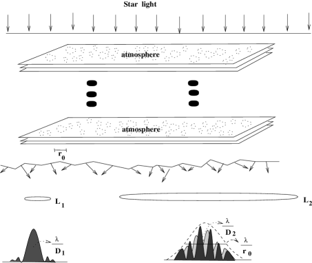
FIG. 1.: Plane-wave propagation through the multiple turbulent layers. ${\tt L}_{1}$ and ${\tt L}_{2}$ represent the small and large telescopes with respective diameters ${\tt D}_{1}$ and ${\tt D}_{2}$.

For a long-exposure through the atmosphere, the resolving power, ${\cal R}$, of any optical telescope can be expressed as,

$${\cal R}=\int{\cal B}({\bf u})\cdot{\cal T}({\bf u})d{\bf u}.$$ (67)

It is limited either by the telescope or by the atmosphere, depending on the relative width of the two functions, ${\cal B}({\bf u})$ and ${\cal T}({\bf u})$.

$${\cal R} = \int{\cal T}({\bf u})d{\bf u}=\frac{\pi}{4}\left(\frac{D}{\lambda}\right)^{2}\,\,\,D\ll r_{\circ}.$$ (69)

$$=\int{\cal B}({\bf u})d{\bf u}=\frac{\pi}{4}\left(\frac{r_{\circ}}{\lambda}\right)^{2}\,\,\,D\gg r_{\circ}.$$

a Fried’s parameter

According to equation (54), ${\cal B}({\bf u})$, can be expressed as,

$${\cal B}({\bf u}) = {\cal B}_{\circ}(\lambda{\bf u})$$ (71)

$$=e^{-\frac{1}{2}\left[2.91k^{2}(\lambda u)^{5/3}\sec\gamma\int{\cal C}_{n}^{2}(z)dz\right]}.$$

Therefore, equation (61) is translated into,

$${\cal R}=(6\pi/5)\left[\frac{1}{2}\left(2.91k^{2}\lambda^{5/3}\sec\gamma\int{\cal C}_{n}^{2}(z)dz\right)\right]^{-6/5}\Gamma(6/5).$$ (72)

Fried, (1966) had introduced the critical diameter $r_{\circ}$, for a telescope; therefore, placing $D=r_{\circ}$ in equation (60), equation (62) takes the following form,

$${\cal B}({\bf u}) = e^{-3.44\left(\lambda u/r_{\circ}\right)^{5/3}}.$$ (73)

$${\cal B}_{\circ}\left({\kern-0.24994pt\hbox{$\xi$}\kern-4.37502pt\kern 0.50003pt\hbox{$\xi$}\kern-4.37502pt\kern-0.24994pt\raise 0.43304pt\hbox{$\xi$}}\right) = e^{-3.44\left(\xi/r_{\circ}\right)^{5/3}}.$$ (74)

The phase structure function (equation 43) across the telescope aperture (Fried, 1966) becomes,

$${\cal D}_{\psi}\left({\kern-0.24994pt\hbox{$\xi$}\kern-4.37502pt\kern 0.50003pt\hbox{$\xi$}\kern-4.37502pt\kern-0.24994pt\raise 0.43304pt\hbox{$\xi$}}\right)=6.88\left(\frac{\xi}{r_{\circ}}\right)^{5/3}.$$ (75)

By replacing the value of ${\cal B}_{\circ}\left({\kern-0.24994pt\hbox{$\xi$}\kern-4.37502pt\kern 0.50003pt\hbox{$\xi$}\kern-4.37502pt\kern-0.24994pt\raise 0.43304pt\hbox{$\xi$}}\right)$, in equation (54), an expression for $r_{\circ}$ in terms of the distribution of the turbulence in the atmosphere is found to be.

$$r_{\circ}=\left[0.423k^{2}\sec\gamma\int{\cal C}_{n}^{2}(z)dz\right]^{-3/5}.$$ (76)

The Fried’s parameter may be thought of as the diameter of telescope that would produce the same diffraction-limited FWHM of a point source image as the atmospheric turbulence would with an infinite-sized mirror.

b Seeing at the telescope site

The major sources of image degradation predominantly comes from thermal and aero-dynamic disturbances in the atmosphere surrounding the telescope and its enclosure. These sources include: (i) convection in and around the building and the dome, obstructed location near the ground, off the surface of the telescope structure, (ii) thermal distortion of the primary and secondary mirrors when they are warmer than the ambient air, (iii) dissipation of heat by the secondary mirror (Zago, 1995), (iv) rise in temperature at the primary mirror cell, and (v) at the focal point causing temperature gradient close to the detector. Degradation in image quality can occur due to opto-mechanical aberrations as well as mechanical vibrations of the optical system.

Various corrective measures have been proposed to improve the seeing. These measures include: (i) insulating the surface of the floors and walls, (ii) introducing an active cooling system to eliminate the heat produced by electric equipment on the telescope and elsewhere in the dome, and (iii) installing a ventilator to generate a downward air flow through the slit to counteract the upward action of the bubbles (Racine, 1984, Ryan and Wood, 1995). Floor-chilling systems to dampen the natural convection have been implemented which keeps the temperature of the primary mirror closer to the air volume (Zago, 1995). Saha and Chinnappan (1999) have found that the average observed $r_{\circ}$ is higher during the later part of the night than the earlier part. This change might indicate that the slowly cooling mirror creates thermal instabilities that decrease slowly during the night.

IV SINGLE APERTURE DIFFRACTION-LIMITED IMAGING

Ever since the development of the SI technique (Labeyrie, 1970), it is widely employed both in the visible, as well as in the infrared (IR) bands at telescopes to decipher diffraction-limited informations. The following sub-sections deal with single aperture speckle imaging and related avenues, other techniques, AO imaging systems, dark speckle imaging, and high resolution sensors.

A Speckle imaging

If a point source is imaged through the telescope by using the pupil function consisting of two sub-apertures ($\theta_{1},\theta_{2}$), corresponding to the two seeing cells separated by a vector $\lambda{\bf u}$, a fringe pattern is produced with narrow spatial frequency bandwidth that moves within broad PSF envelope; with increasing distance between the sub-apertures, the fringes move with an increasingly larger amplitude. The introduction of a third sub-aperture gives three pairs of sub-apertures and yields the appearance of three intersecting patterns of moving fringes. Covering the telescope aperture with $r_{\circ}$-sized sub-apertures synthesizes a filled aperture ${\it p}_{j}$ (each pair of them, ${\it p}_{n},{\it p}_{m}$, is separated by a baseline) interferometer. The intensity at the focal-plane, ${\cal I}$, according to the diffraction theory (Born and Wolf, 1984), is determined by the expression,

$${\cal I}=\sum_{n,m}<\Psi_{n}\Psi^{\ast}_{m}>.$$ (77)

The term, $\Psi_{n}\Psi^{\ast}_{m}$, is multiplied by $e^{i\psi}$, where $\psi$ is the random instantaneous shift in the fringe pattern. Each sub-aperture is small enough for the field to be coherent over its extent. Atmospheric turbulence does not affect the contrast of the fringes produced but introduces phase delays. If the integration time is shorter than the evolution time of the phase inhomogeneities, the interference fringes are preserved but their phases are randomly distorted, which produces ‘speckles’. (The formation of speckles stems from the summation of coherent vibrations having random characteristics. It can be modeled as a 2-dimensional random walk with Fresnel’s vector representation of vibrations). Each speckle covers an area of the same order of magnitude as the Airy disc of the telescope. The number of correlation cells is proportional to the square of $D/r_{\circ}$ and the number of photons, $N_{p}$, per speckle is independent of its diameter. The lifetime of speckles, $\tau_{\circ}\sim r_{\circ}/\Delta\nu$, where $\Delta\nu$ is the velocity dispersion in the turbulent seeing layers across the line of sight.

The structure of the speckle pattern changes randomly over a short interval of time. The sum of several such statistically uncorrelated patterns from a point source can result in a uniform patch of light a few arcseconds (^′′) wide. Figures 2 and 3 depict the speckles of a binary star HR4689 and the results of summing 128 specklegrams, respectively. Averaging $\widehat{\cal I}({\bf u})$ over many frames, the resultant for frequencies greater than $r_{\circ}/\lambda$, tends to zero because the phase-difference, $\theta_{1}-\theta_{2}$, mod $2\pi$, between the two apertures is distributed uniformly between $\pm\pi$, with zero mean. The Fourier component performs a random walk in the complex plane and averages to zero:

$$<\widehat{\cal I}{\bf(u)}>=0,\ \ \ \ u>r_{\circ}/\lambda.$$ (78)

FIG. 2.: Specklegram of a binary star, HR4689 obtained at the VBT, Kavalur, India.

FIG. 3.: The result of summing 128 specklegrams of HR4689 demonstrating the destructions of finer details of the image by the atmospheric turbulence.

In general, a high quantum efficiency detector is needed to record magnified short-exposure images for such observation. To compensate for atmospherically induced dispersion at zenith angles larger than a few degrees, either a counter-rotating computer-controlled dispersion-correcting prism or a narrow-bandwidth filter is used.

1 Speckle interferometry (SI)

Speckle interferometry estimates a ‘power spectrum’ which is the ensemble average of the squared modulus of an ensemble of FT from a set of specklegrams, ${\cal I}_{k}({\bf x}),k=t_{1},t_{2},t_{3},\ldots,t_{M}$. The intensity of the image, ${\cal I}({\bf x})$, in the case of quasi-monochromatic incoherent source can be expressed as,

$${\cal I}({\bf x})=\int{\cal O}({\bf x}^{\prime}){\cal S}({\bf x}-{\bf x}^{\prime})d{\bf x}^{\prime}.$$ (79)

where ${\cal O}({\bf x}^{\prime})$, is an object at a point anywhere in the field of view.

The variability of the corrugated wavefront yields ‘speckle boiling’ and is the source of speckle noise that arises from difference in registration between the evolving speckle pattern and the boundary of the PSF area in the focal-plane. These specklegrams have additive noise contamination, ${\cal N}_{j}({\bf x})$, which includes all additive measurement of uncertainties. This may be in the form of (i) photon statistics noise, and (ii) all distortions from the idealized iso-planatic model represented by the convolution of ${\cal O}({\bf x})$ with ${\cal S}({\bf x})$ that includes non-linear geometrical distortions. For each of the short-exposure instantaneous records, the imaging equation applies,

$${\cal I}{(\bf x)}={\cal O}{(\bf x)}\star{\cal S}{(\bf x)}+{\cal N}({\bf x}),$$ (80)

Denoting $\widehat{\cal N}({\bf u})$, for the noise spectrum. the Fourier space relationship between object and the image is

$$\widehat{\cal I}({\bf u})=\widehat{\cal O}({\bf u})\cdot\widehat{\cal S}({\bf u})+\widehat{\cal N}({\bf u}).$$ (81)

Taking the modulus square of the expression and averaging over many frames, the average image power spectrum is,

$$<|\widehat{\cal I}({\bf u})|^{2}>=|\widehat{\cal O}({\bf u})|^{2}\cdot<|\widehat{\cal S}({\bf u})|^{2}>+<|\widehat{\cal N}({\bf u})|^{2}>.$$ (82)

Since $|\widehat{\cal S}({\bf u})|^{2}$ is a random function in which the detail is continuously changing, its ensemble average becomes smoother.

By the Wiener-Khintchine theorem (Mendel and Wolf, 1995), the inverse FT of equation (73) gives the autocorrelation of the object, ${\cal A}[{\cal O}{\bf(x)}]$.

$${\cal A}[{\cal O}{\bf(x)}]={\cal F}^{-}[|\widehat{\cal O}{\bf(u)}|^{2}],$$ (83)

In this technique, the atmospheric phase contribution is eliminated but the averaged signal is non-zero, i.e.,

$$<\widehat{\cal I}^{\cal A}({\bf u})>\neq 0.$$ (84)

The argument of the equation (72) is given by the expression,

$$arg|\widehat{\cal I}{\bf(u)}|^{2} = \psi({\bf u})+\theta_{1}-\theta_{2}+\psi{\bf(-u)}-\theta_{1}+\theta_{2}$$ (86)

$$=0.$$

The transfer function of ${\cal S}({\bf x})$, is generally estimated by calculating the power spectrum of the instantaneous intensity from an unresolved star. Saha and Maitra (2001) developed an algorithm, where a Wiener parameter, $w_{1}$, is added to PSF power spectrum. The classic Wiener filter that resulted from electronic information theory where diffraction-limits do not mean much, is meant to deal with signal dependent ‘colored’ noise. In practice, this term is usually just a constant, a ‘noise control parameter’ whose scale is estimated from the noise power spectrum. In this case, it assumes that the noise is white and that one can estimate its scale in regions of the power spectrum where the signal is zero (outside the diffraction-limit for an imaging system).

$$|\widehat{O}{\bf(u)}|^{2}=\frac{<|\widehat{I}{\bf(u)}|^{2}>}{[<|\widehat{S}{\bf(u)}|^{2}>+w_{1}]}.$$ (87)

The SI technique in the case of the components in a group of stars retrieves the separation, position angle with 180^∘ ambiguity, and the relative magnitude difference at low light levels. Figure 4 depicts the autocorrelation of a binary system, HR4689. Another algorithm called directed vector autocorrelation (DVA) method is found to be effective in eliminating the 180^∘ ambiguity (Bagnuolo et al. 1992).

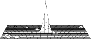
FIG. 4.: Autocorrelation of a binary system, HR4689; the second star in the binary is one of the two distinct bumps and symmetrically placed on either side of the main peak. The bumps at the edge of the figure are the artifacts.

2 Speckle holography

If a reference point source is available within the iso-planatic patch ($\sim 7^{\prime\prime}$), it is used as a key to reconstruct the target in the same way as a reference coherent beam is employed in holographic reconstruction (Liu and Lohmann, 1973). Let the point source be represented by a Dirac impulse, $A_{\circ}\delta({\bf x})$ at the origin and ${\cal O}_{1}({\bf x})$ be the nearby object to be reconstructed. The intensity distribution in the field of view is

$${\cal O}({\bf x})=A_{\circ}\delta({\bf x})+{\cal O}_{1}({\bf x}).$$ (88)

The squared modulus of its FT is derived as,

$$|\widehat{\cal O}({\bf u})|^{2}=A_{\circ}^{2}+A_{\circ}\widehat{\cal O}_{1}({\bf u})+A_{\circ}\widehat{\cal O}_{1}^{\ast}({\bf u})+\widehat{\cal O}_{1}({\bf u})\widehat{\cal O}_{1}^{\ast}({\bf u}).$$ (89)

The inverse FT of this equation translates into,

$${\cal A}[{\cal O}{(\bf x)}]=A_{\circ}^{2}\delta{(\bf x)}+A_{\circ}{\cal O}_{1}{(\bf x)}+A_{\circ}{\cal O}_{1}{(\bf-x)}+{\cal A}[{{\cal O}_{1}}{(\bf x)}],$$ (90)

The first and the last terms in equation (80) are centered at the origin. If the object is far enough from the reference source, ${\cal O}({\bf x})$, its mirror image, ${\cal O}{(\bf-x)}$, is therefore recovered apart from a 180^∘ rotation ambiguity.

3 Differential speckle interferometry

Differential speckle interferometry (DSI) is a method to observe the objects in different spectral channels simultaneously and to compute the average cross-correlation of pairs of speckle images (Beckers, 1982). Let ${\cal O}_{1}{(\bf x)}$ and ${\cal O}_{2}{(\bf x)}$, be respectively the source brightness distributions at $\lambda_{1}$ and $\lambda_{2}$, and ${\cal I}_{1}{(\bf x)}$ and ${\cal I}_{2}{(\bf x)}$, their associated instantaneous image intensity distributions. The relation between the object and the image in the Fourier space becomes,

$$\widehat{\cal I}_{1}({\bf u}) = \widehat{\cal O}_{1}({\bf u})\cdot\widehat{\cal S}_{1}({\bf u}),$$ (91)

$$\widehat{\cal I}_{2}({\bf u}) = \widehat{\cal O}_{2}({\bf u})\cdot\widehat{\cal S}_{2}({\bf u}),$$ (92)

where $\widehat{\cal S}_{1}{(\bf u)}$ and $\widehat{\cal S}_{2}{(\bf u)}$ are the related transfer functions. The average cross-spectrum is given by,

$$<\widehat{\cal I}_{1}{(\bf u)}\widehat{\cal I}_{2}^{\ast}{(\bf u)}>=\widehat{\cal O}_{1}{(\bf u)}\widehat{\cal O}_{2}^{\ast}{(\bf u)}\cdot<\widehat{\cal S}_{1}{(\bf u)}\widehat{\cal S}_{2}^{\ast}({\bf u})>.$$ (93)

The transfer function, $<\widehat{\cal S}_{1}{(\bf u)}\widehat{\cal S}_{2}^{\ast}{(\bf u)}>$, can be calibrated on the reference point source for which, $<\widehat{\cal O}_{1}{(\bf u)}>=<\widehat{\cal O}_{2}{(\bf u)}>=1$. If the two spectral windows are close enough ($\Delta\lambda/\lambda\ll r_{\circ}/D$), the instantaneous transfer function is assumed to be identical in both the channels [${\cal S}_{1}={\cal S}_{2}={\cal S}$]. Therefore, equation (83) becomes,

$$\widehat{\cal O}_{1}({\bf u}) = \frac{<\widehat{\cal I}_{1}({\bf u})\widehat{\cal I}_{2}^{\ast}({\bf u})>}{\widehat{\cal O}_{2}^{\ast}({\bf u})<|\widehat{\cal S}({\bf u})|^{2}>}$$ (95)

$$=\widehat{\cal O}_{2}({\bf u})\frac{<\widehat{\cal I}_{1}({\bf u})\widehat{\cal I}_{2}^{\ast}({\bf u})>}{<|\widehat{\cal I}_{2}({\bf u})|^{2}>}.$$

The noise contributions from two different detectors are uncorrelated, and thereby their contributions cancel out. The DSI estimates the ratio, $\widehat{\cal O}_{1}({\bf u})/\widehat{\cal O}_{2}({\bf u})$ and the differential image, ${\cal D}_{\cal I}({\bf x})$, is obtained by performing an inverse FT of this ratio,

$${\cal D}_{\cal I}({\bf x})={\cal F}^{-1}\left[\frac{<\widehat{\cal I}_{1}({\bf u})\widehat{\cal I}_{2}^{\ast}({\bf u})>}{<|\widehat{\cal I}_{2}({\bf u})|^{2}>}\right],$$ (96)

where ${\cal D}_{\cal I}({\bf x})$ represents an image of the object in the emission feature having the resolution of the object imaged in the continuum.

4 Speckles and shadow bands

When any planetary body of a notable size passes in front of a star, the light coming from the latter is occulted. The profiles of stellar occultations by the Moon show diffraction patterns as the star is being occulted, provided the data is recorded at high time resolution. The method remains useful because of the extraordinary geometric precision it provides. The notable advantage of occultation of binary stars is that it can determine relative intensities and measure the separations comparable to those measured by long baseline interferometers. Speckle surveys have resolved known occulting binaries down to a separation of about $<$ 0.025^′′ (Mason, 1996). Further, this method provides a means of determining the limiting magnitude difference of SI. The shortcomings of this technique may be noted due to its singular nature: the object may not occult again until one Saros cycle later (18.6 yr), and must be limited to a belt of the sky (10% of the celestial sphere).

5 Speckle spectroscopy

The application of the SI technique to speckle spectroscopic observations enables one to obtain spectral resolution with high spatial resolution of astronomical objects simultaneously. The intensity distribution, ${\cal W}({\bf x})$, of an instantaneous objective prism speckle spectrogram is expressed as,

$${\cal W}({\bf x})=\sum_{m}{\cal O}_{m}({\bf x}-{\bf x}_{m})\star{\cal G}_{m}({\bf x})\star{\cal S}({\bf x}),$$ (97)

where ${\cal O}_{m}({\bf x}-{\bf x}_{m})$ denotes the intensity of m^th object pixel and ${\cal G}_{m}({\bf x})$ is the spectrum of the object pixel. In the narrow wavelength bands ($<$30 nm), the PSF, ${\cal S}({\bf x})$, is wavelength independent. The objective prism spectrum, $\sum_{m}{\cal O}_{m}({\bf x}-{\bf x}_{m})\star{\cal G}_{m}(\bf x)$, can be reconstructed from the speckle spectrograms.

In a speckle spectrograph, either a prism or a grism can be employed to disperse 1-d specklegrams (Grieger et al. 1988). An imaging spectrometer uses two synchronized detectors to record the dispersed speckle pattern and the specklegrams of the object (Baba, Kuwamura et al. 1994); a reflection grating acts as disperser.

6 Speckle polarimetry

In general, radiation is polarized and the measurement of polarization parameters is important in understanding of the emission mechanisms. Processes such as electric and magnetic fields, scattering, chemical interactions, molecular structure, and mechanical stress cause changes in the polarization state of an optical beam. Applications relying on the study of these changes cover a vast area, among them are astrophysics and molecular biology. The importance of such observations in astronomy is to obtain information such as the size and shapes of dust envelopes around stars, the size and shape of the dust grains, and magnetic fields. Among other astronomical objectives worth investigating are: (i) the wavelength dependence of the degree of polarization and the rotation of the position angle in stars with extended atmospheres, (ii) the wavelength dependence of the degree of polarization and position angle of light emitted by stars present in very young ($\leq 2\times 10^{6}$ years) clusters and associations.

The modified incident polarization caused by the reflection of a mirror is characterized by two parameters: (i) the ratio between the reflection coefficients of the electric vector components which are perpendicular and parallel to the plane of incidence, known as $s$ and $p$ components respectively, (ii) the relative phase-shift between these electric vibrations. The effect on the statistics of a speckle pattern is the degree of depolarization caused by the scattering at the surface. If the light is depolarized, the resulting speckle field is considered to be the sum of two component speckle fields produced by scattered light polarized in two orthogonal directions. The intensity at any point is the sum of the intensities of the component speckle patterns (Goodman, 1975). These patterns are partially correlated; therefore, a polarizer that transmits one of the component speckle patterns is used in the speckle camera system (Falcke et al. 1996). The advantage of using a speckle camera over a conventional imaging polarimeter is that it helps in monitoring the short-time variability of the atmospheric transmission.

7 Speckle imaging of extended objects

Image recovery is relatively simple where the target is a point source. Nevertheless, interferometric observations can reveal the fundamental processes on the Sun that take place on sub-arcsecond scales concerning convection and magnetic fields. The limitations come from (i) the rapid evolution of solar granulation that prevents the collection of long sequences of specklegrams for reconstruction, (ii) the lack of efficient detectors to record a large number of frames within the stipulated time before the structure changes. Another major problem of reconstructing images comes from difficulty in estimating the PSF due to the lack of a reference point source. The spectral ratio technique (Von der Lühe, 1984), which is based on a comparison between long and short-exposure images, has been employed (Wilken et al. 1997) to derive Fried’s parameter. Models of the speckle transfer function (Korff, 1973) and of average short-exposure MTF have also been applied to compare the observed spectral ratios with theoretical values. High resolution solar images obtained during partial solar eclipse may help in estimating the seeing effect (Callados and Vàzquez, 1987). The limb of the moon eclipsing the sun provides a sharp edge as a reference object. The intensity profile falls off sharply at the limb. The departure of this fall off gives an indirect estimate of the atmospheric PSF.

B Other techniques

Several other methods, viz., pupil-plane techniques such as wavefront shearing interferometry, phase-closure methods, and phase-diversity techniques are also employed at single telescope in order to obtain diffraction-limited information.

1 Shearing interferometry

Shearing interferometers make use of the principle of self referencing, that is, they combine the wavefront with a shifted version of itself to form interferences. Fringes are produced by two partially or totally superimposed pupil images created by introducing a beam splitter. At each point, interference occurs from the combination of only two points on the wavefronts at a given baseline, and therefore, behaves as an array of Michelson-Fizeau interferometers. An important property of these interferometers is their ability to work with partially coherent light, which offers better S/N ratio on bright sources, and is insensitive to calibration errors due to seeing fluctuations and telescope aberrations. A rotational shear interferometer was used at the telescope to map the visibility of fringes produced by $\alpha$ Ori (Roddier and Roddier, 1988). In this technique, the 2-d FT is obtained by rotating one pupil image about the optical axis by a small angle with respect to the other. If the rotation axis coincides with the center of the pupil, the two images overlap. All the object Fourier components within a telescope’s diffraction cutoff frequency are measured simultaneously.

2 Phase-closure methods

The phase of the visibility may be deduced from a closure-phase that is insensitive to the atmospherically induced random phase errors, as well as to the permanent phase errors introduced by the imaging systems (Jennison, 1958) using three telescopes. The observed phases, $\psi_{ij}$, on the different baselines contain the phases of the source Fourier components $\psi_{0,ij}$ and also the error terms, $\theta_{j},\theta_{i}$, introduced by errors at the individual antennas and by the atmospheric variations at each antenna. The observed fringes are represented by the following equations,

$$\psi_{12} = \psi_{0,12}+\theta_{2}-\theta_{1}.$$ (98)

$$\psi_{23} = \psi_{0,23}+\theta_{3}-\theta_{2}.$$ (99)

$$\psi_{31} = \psi_{0,31}+\theta_{1}-\theta_{3}.$$ (100)

where the subscripts refer to the antennae at each end of a particular baseline. The closure phase, $\beta_{123}$ is the sum of phases of the source Fourier components and is derived as,

$$\beta_{123} = \psi_{12}+\psi_{23}+\psi_{31},$$ (102)

$$=\psi_{0,12}+\psi_{0,23}+\psi_{0,31}.$$

This equation implies cancellations of the antennae phase errors. Using the measured closure phases and amplitudes as observables, the object phases are determined (mostly by least square techniques, viz., singular value decomposition, conjugate gradient method). From the estimated object phases and the calibrated amplitudes, the degraded image is reconstructed.

Baldwin et al. (1986) reported the measurements of the closure-phases obtained at a high light level with a three hole aperture mask set in the pupil-plane of the telescope. The non-redundant aperture masking method, in which the short-exposure images are taken through a multi-aperture screen, has several advantages. These are: (i) an improvement of signal-to-noise (S/N) ratios for the individual visibility and closure-phase measurements, (ii) attainment of the maximum possible angular resolution by using the longest baselines, and (iii) built-in delay to observe objects at low declinations. But the system is restricted to high light levels, because the instantaneous coverage of spatial frequencies is sparse and most of the available light is discarded.

3 Phase-diversity imaging

Phase-diversity (Gonsalves, 1982, Paxman et al. 1992) is a post-collection technique that uses a number of intensity distributions encoded by known aberrations for restoring high spatial resolution detail while imaging in the presence of atmospheric turbulence. The phase aberrations are estimated from two simultaneously recorded images. Phase-diverse speckle is an extension of this technique, whereby a time sequence of short-exposure image pairs is detected at different positions in focus and out of focus near the focal-plane. Incident energy is split into two channels by a simple beam splitter: one is collected at a conventional focal-plane, the other is defocussed (by a known amount) and a second detector array permits the instantaneous collection of the latter. It is less susceptible to the systematic errors caused by the optical hardware, and is found to be more appealing in astronomy (Baba, Tomita et al. 1994, Seldin and Paxman, 1994).

C Adaptive-optics (AO)

Significant technological innovations over the past several years have made it possible to correct perturbations in the wavefronts in real time by incorporating a controllable phase distortion in the light path, which is opposite to that introduced by the atmosphere (Babcock, 1953, Rousset et al. 1990). This technique has advantages over post-detection image restoration techniques that are limited by noise. Adaptive-optics (AO) systems are employed in other branches of physics as well. Liang et al. (1997) have constructed a camera equipped with adaptive-optics that allows one to image a microscopic size of single cell in the living human retina. They have shown that a human eye with adaptive-optics correction can resolve fine gratings that are invisible to the unaided eye. AO systems are useful for spectroscopic observations, as well as for low light level imaging with future very large telescopes, and ground-based LBOIs.

1 Greenwood frequency

Turbulence cells are blown by wind across the telescope aperture, hence, the wind velocity dictates the speed with which a corrective action must be taken. Greenwood (1977) derives the mean square residual wavefront error as a function of servoloop bandwidth for a first order controller, which is given by,

$$\sigma^{2}_{cl}=\left(\frac{{\it f}_{G}}{{\it f}_{3db}}\right)^{5/3}\,\,{rad}^{2},$$ (103)

where ${\it f}_{3db}$ is the closed loop bandwidth of the wavefront compensator and ${\it f}_{G}$ the Greenwood frequency that is defined by the relation,

$${\it f}_{G}=\frac{0.426{\it v}}{r_{\circ}},$$ (104)

where ${\it v}$ is the wind velocity in the turbulent layer of air. For imaging in near-IR to ultraviolet, the AO system bandwidths need to have a response time of order several hundreds to 1 KHz. It is easier to achieve diffraction-limited information using AO systems at longer wavelengths since $r_{\circ}$ is proportional to the six-fifths power of the wavelength,

$$r_{\circ}\propto\lambda^{6/5}.$$ (105)

The above equation (94) implies that the width of seeing limited images, $1.22\lambda/r_{\circ}\propto\lambda^{-1/5}$ varies with $\lambda$. The number of degrees of freedom, i.e., the number of actuators on the deformable mirror (DM) and the number of sub-aperture in the wavefront sensor, in an AO system should be determined by the following equation,

$$(D/r_{\circ})^{2}\propto\lambda^{-12/5}.$$ (106)

2 AO imaging system

The required components for implementing an AO system are wavefront sensing, wavefront phase error computation and a flexible mirror whose surface is electronically controlled in real time to create a conjugate surface enabling compensation of the wavefront distortion (Roggemann et al. 1997 and references therein). In order to remove the low frequency tilt error, generally the incoming collimated beam is fed by a tip-tilt mirror. After traveling further, it reflects off of a DM that eliminates high frequency wavefront errors. A beam-splitter devides the beam into two parts: one is directed to the wavefront sensor to measure the residual error in the wavefront and to provide information to the actuator control computer to compute the DM actuator voltages and the other is focused to form an image.

Implementation of the dynamically controlled active optical components consisting of a tip-tilt mirror system in conjunction with closed-loop control electronics has several advantages: (i) conceptually the system is simple, (ii) fainter guide stars increase the sky coverage, and (iii) field of view is wider (Glindemann, 1997). These systems are limited to two Zernike modes (x and y tilt), while a higher order system compensating many Zernike mode (Zernike polynomials are an orthogonal expansion over unit circle) is required to remove high frequency errors.

A variety of DMs have been developed for the applications of (i) high energy laser focusing, (ii) laser cavity control, (iii) compensated imagery through atmospheric turbulence etc. Several wavefront sensors such as (i) lateral shearing interferometer, (ii) Shack-Hartman (SH) sensor, and (iii) the curvature sensor are in use as well. The technical details of these DMs and sensors are enumerated in the recent literatures (Roggemann et al. 1997, Roddier, 1999, and Saha, 1999).

The phase reconstruction method finds the relationship between the measurements and the unknown values of the wavefronts and can be categorized as being either zonal or modal, depending on whether the estimate is either a phase value in a local zone or a coefficient of an aperture function (Rousset, 1999). In the case of curvature sensing, the computed sensor signals are multiplied by a control matrix to convert wavefront slopes to actuator control signals, the output of which are the increments to be applied to the control voltages on the DM. A conjugate shape is created using these data by controlling a DM.

The real time computation of the wavefront error, as well as correction of wavefront distortion involves digital manipulation of wavefront sensor data in the wavefront sensor processor, the re-constructor and the low-pass filter, and converting to analog drive signals for the DM actuators. The functions are (i) to compute sub-aperture gradients, phases at the corners of each sub-aperture, low-pass filter phases, and (ii) to provide actuator offsets to compensate the fixed optical system errors and real time actuator commands for wavefront corrections.

3 Artificial source

An AO system requires a reference source to monitor the atmospheric aberrations for measuring the wavefront errors, as well as for mapping the phase on the entrance pupil. It is generally not possible to find a sufficiently bright reference star close enough to a target star. In order to alleviate this limitation, many observatories are currently implementing the artificial laser guide star (Ragazzoni and Bonnacini, 1996, Racine et al. 1996, Lloyd-Hart et al. 1998). However, the best results are still obtained with natural guide stars.

An artificial guide star can be obtained using either the resonance scattering by sodium in the mesosphere at 90 km (Foy and Labeyrie, 1985) or Rayleigh scattering between 10 and 20 km altitude (Fugate et al. 1994). A pulsed laser (tuned to the sodium $D_{2}$ line to excite sodium atom) is used to produce a bright compact glow in the upper atmosphere. Concerning the flux backscattered by a laser shot, Thompson and Gardner (1988) stressed the importance of investigating two basic problems: (i) the cone effect which arises due to the parallax between the remote astronomical source and artificial source, and (ii) the angular anisoplanatic effects. These effects can be restored by imaging the various turbulent layers of the atmosphere onto different adaptive mirrors (Tallon et al. 1988). Scattering of the upward propagating laser beam is due to Rayleigh scattering, mostly by $N_{2}$ molecules. Mie scattering by aerosol or cirrus clouds may be important at lower altitudes but are usually variable and transient.

4 Multi-conjugate adaptive-optics

Multi-conjugate AO system enables near-uniform compensation for the atmospheric turbulence over considerably larger field of view than can be corrected with normal AO system. This method employs an ensemble of guide stars that allows for 3-d tomography of the atmospheric turbulence and a number of altitude-conjugate DMs to extend the compensated field of view. However, its performances depends on the quality of the wavefront sensing of the individual layers. Ragazzoni et al. (2000) have demonstrated this type of tomography. This new technique pushes the detection limit by $\sim$1.7 mag on unresolved objects with respect to seeing limited images; it also minimizes the cone effect. This technique will be useful for the extremely large telescopes of 100 m class, e.g., the OverWhelmingly Large (OWL) telescope (Dierickx and Gilmozzi, 1999). However, the limitations are mainly related to the finite number of actuators in a DM, wavefront sensors, and guide stars.

5 Adaptive secondary mirrors

The usage of a adaptive secondary mirror (ASM) for corrections making relay optics obsolete that are required to conjugate a DM at a reimaged pupil, as well as to minimize thermal emission is a new key innovation (Bruns et al. 1997). The other notable advantages are (i) enhanced photon throughput that measures the proportion of light which is transmitted through an optical set-up, (ii) introduction of negligible extra IR emissivity, (iii) causes no extra polarization, and (iv) non-addition of reflective losses (Lee et al. 2000). Due to the interactuator spacing, the resonant frequency of such a mirror may be lower than the AO bandwidth. The ASM system uses a SH sensor with an array of small lenslets, which adds two extra refractive surfaces to the wavefront sensor optical beam (Lloyd-Hart, 2000). An $f/15$ AO secondary with 336 actuators is in the final stages of testing and will be installed on the 6.5 m Telescope of MMT observatory, Mt. Hopkins, Arizona in 2002 (Wehinger, 2001).

6 High resolution coronagraphy

The relevance of using coronagraphy in imaging or spectroscopy of faint structure near a bright object can be noted in terms of reducing the light coming from the central star, and filtering out of the light at low spatial frequency; the remaining light at the edge of the pupil corresponds to high frequencies. A coronagraph reduces off-axis light from an on-axis source with an occulting stop in the image-plane as well as with a matched Lyot stop in the next pupil plane. While using the former stop the size of the latter pupil should be chosen carefully to find the best trade-off between the throughput and image suppression. The limitations come from the light diffracted by the telescope and instrument optics. Coronagraphy with dynamic range can be a powerful tool for direct imaging of extra-solar planets. Nakajima (1994) estimates that imaging with such a method with a low order AO system in a 6.5 m telescope could detect Jupiter-size extra-solar planets at separation $\sim$1.5^′′ with S/N of 3 in 10⁴ s. Rouan et al. (2000) describes a four-quadrant phase-mask coronagraph where a detection at a contrast of more than 8 mag difference between a star and a planet is feasible.

D Dark speckle method

The dark speckle method uses the randomly moving dark zones between speckles $-$ ‘dark speckles’. It exploits the light cancellation effect in a random coherent field; highly destructive interferences that depict near black spots in the speckle pattern (Labeyrie, 1995) may occur occasionally. The aim of this method is to detect faint objects around a star when the difference of magnitude is significant. If a dark speckle is at the location of the companion in the image, the companion emits enough light to reveal itself.

The required system consists of a telescope with an AO system, a coronagraph, a Wynne corrector, and a fast photon-counting camera with a low dark noise. If a pixel of the photon-counting camera is illuminated by the star only (in the Airy rings area), because of the AO system, the number of photons in each pixel, for a given interval (frame), is statistically given by a Bose-Einstein distribution. The number of photons per frame in the central peak of the image of a point source obeys a classical Poisson distribution. For the pixels containing the image of the companion, the number of photons, resulting from both the star and the companion, is given by a different distribution (computed by mixing Bose-Einstein and Poisson distributions). One noticeable property is that the probability to get zero photons in a frame is very low for the pixels containing the image of the companion, and much higher for the pixels containing only the contribution from the star. Therefore, if the ‘no photon in the frame’ events for each pixel is counted, and for a very large number of frames, a ‘dark map’ can be built that will show the pixels for which the distribution of the number of photons is not Bose-Einstein type, therefore revealing the location of a faint companion. The role of the Wynne corrector is to give residual speckles the same size regardless the wavelength. Otherwise, dark speckles at a given wavelength would be overlapped by bright speckles at other wavelengths. With the current technology, by means of the dark speckle technique at a 3.6 m telescope should allow detection of a companion with $\Delta m_{k}\approx$6-7 mag. Figures 5 and 6 depict the coronagraphic images of the binary stars, HD192876 and HD222493, respectively (Boccaletti et al. 2001); the data were obtained with ADONIS in the K band (2.2 $\mu$m) on the European Southern Observatory’s (ESO) 3.6 m telescope. Due to the lack of a perfect detector (no read-out noise) at near-IR band, every pixel under the defined threshold (a few times the read-out noise) is accounted as a dark speckle.

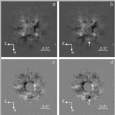
FIG. 5.: Coronagraphic images of the star HD192876 (Courtesy: A. Boccaletti). An artificial companion is added to the data to assess the detection threshold ($\Delta m_{K}$=6.0 mag, $\rho=0.65"$); (a) direct image : co-addition of 400$\times$60 ms frames, (b) same as (a) with a $\Delta m_{K}$=6.0 mag companion (SNR 1.8), (c) dark speckle analysis, and (d) dark speckle analysis with the companion (SNR 4.8); the detection threshold is about $\Delta m_{K}$=7.5 mag on that image, i.e an improvement of 1.5 mag compared to the direct image (Boccaletti et al. 2001).

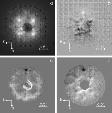
FIG. 6.: Coronagraphic images of the binary star HD222493 ($\Delta m_{K}$=3.8 mag, $\rho=0.89"$); (a) direct image: co-addition of 600$\times$60 ms frames, (b) subtraction of the direct image with a reference star (SNR=14.6), (c) dark speckle analysis (constant threshold) and subtraction of a reference star, and (d) dark speckle analysis (radial threshold) and subtraction of a reference star (SNR=26.7) (Boccaletti et al. 2001: Courtesy: A. Boccaletti).

Phase boiling, a relatively new technique that consists of adding a small amount of white noise to the actuators in order to get a fast temporal decorrelation of the speckles during long-exposure acquisition, may produce better results. Aime (2000) has computed the S/N ratio for two different cases: short-exposure and long-exposure. According to him, even with an electron-noise limited detector like a CCD or a near-IR camera multi-object spectrometer (NICMOS), the latter can provide better results if the halo has its residual speckles smoothed by fast residual ‘seeing’ acting during the long-exposure than building a dark map from short-exposures in the photon-counting mode. Artificial very fast seeing can also be generated by applying fast random noise to the actuators, at amplitude levels comparable to the residual seeing left over by the AO system.

The question is, what is easiest: dark speckle analysis or a ‘hyper-turbulated’ long-exposure? Labeyrie (2000) made simulations supporting the Aime’s (2000) results. Boccaletti (2001) has compared the dark speckle signal-to-noise ratio (SNR) with the long-exposure SNR (Angel, 1994). The speckle lifetime has to be of order 0.1 ms. Currently it is impossible to drive a DM at this frequency (10 kHz). With the 5 m Palomar telescope Boccaletti (2001) tried to smooth the speckle pattern by adding a straightforward random noise on the actuators (the DM is equipped with 241 actuators) at maximum speed of 500 Hz. Effectively, the halo is smoothed, but its intensity is also increased, so that the companion SNR is actually decreased. Blurring the speckle pattern would probably require wavefront sensor telemetry; implementation of a hyper-turbulated long-exposure at the Palomar is still under study (Boccaletti, 2001).

E High resolution sensors

All the techniques that are described above require a high quality sensor so as to enable one to obtain snap shots with a very high time resolution of the order of (i) frame integration of 50 Hz, or (ii) photon recording rates of a few MHz. The performance relies on the characteristics of such sensors, e.g., (i) the spectral bandwidth, (ii) the quantum efficiency, (iii) the detector noise that includes dark current, read-out and amplifier noise, (iv) the time lag due to the read-out of the detector, and (v) the array size and the spatial resolution.

1 Frame-transfer camera systems

The frame-transfer intensified CCD (ICCD) camera employs micro-channel plate (MCP) as an intensifier. The photoelectron is accelerated into a channel of the MCP releasing secondaries and producing an output charge cloud of about $10^{3}-10^{4}$ electrons with 5 - 10 kilovolt (KV) potential. With further applied potential of $\sim$5 - 7 KV, these electrons are accelerated to impact a phosphor, thus producing an output pulse of $\sim 10^{5}$ photons. These photons are directed to the CCD by fiber optic coupling. The main disadvantage of such system is the poor gain statistics results in the introduction of a noise factor between 2 and 3.5. Recent development of a non-intensified CCD device which effectively reduces readout noise to less than one electron rms has enabled substantial internal gain within the CCD before the signal reaches the output amplifier (Mackay et al. 2001). Such a detector, although the photon counting performance appears moderate for the moment, shows promise for quantitative measurement of diffraction-limited stellar images.

2 Photon-counting detectors

The marked advantage of a photon-counting system is that of reading the signal a posteriori to optimize the correlation time of short-exposures in order to overcome the loss of fringe visibility due to the speckle lifetime; the typical values for an object of m_v = 12 over a field of 2.5^′′ are less than 50 photons/ms through a narrow-band filter. The other notable features are, (i) capability of determining the position of a detected photon, (ii) ability to register individual photons with equal statistical weight and produces signal pulse (with dead time of a few ns), and (iii) low dark noise.

The major short comings of the photon-counting system that is based on frame integration (Blazit, 1986) arise from the (i) calculations of the coordinates which are hardware-limited, and (ii) limited dynamic range of the detector. Non-detectability of a pair of photons closer than a minimum separation by the detector yields a loss in high frequency information; this, in turn, produces a hole in the center of the autocorrelation $-$ Centreur hole, resulting in the degradation of the power spectra or bispectra (FT of triple correlation) of speckle images.

Several 2-d photon-counting sensors that allow recording of the position and time of arrival of each detected photons have been developed such as, (i) precision Analog Photon Address (PAPA; Papaliolios et al. 1985), (ii) resistive anode position detector (Clampin et al. 1988), (iii) multi anode micro-channel array (MAMA; Timothy, 1993), (iv) wedge-and-strip anodes, (v) delay-line anodes, (vi) silicon anode detector etc. Baring PAPA which is based on a high gain image intensifier and a set of photomultiplier tubes, these sensors detect the charge cloud from a high gain MCP. They provide spatial event information by means of the position sensitive readout set-up; the encoding systems identify each event’s location. The short-comings of the MCPs are notably due to its local dead-time which essentially restricts the conditions for use of these detectors for high spatial resolution applications. These constraints are also related with the luminous intensity and the pixel size.

3 Infrared sensors

In the infrared band, no photon-counting is possible with the current technology. Nevertheless, a near-IR focal-plane array, NICMOS, has been developed. It consists of 256$\times$256 integrating detectors organized in four independent 128$\times$128 quadrants and is fabricated in HgCdTe grown on a saphire substrate that is very rugged and provides a good thermal contraction match to silicon multiplexer (Cooper et al. 1993). The typical NICMOS3 FPAs have read noise less than 35 e- with less than 1 e-/sec detector dark current at 77 K and broadband quantum efficiency is better than 50% in the range of 0.8 to 2.5 $\mu$m.

V DILUTE-APERTURE INTERFEROMETRY

Modern technology has solved many of the problems that were pioneered by Michelson and Pease (1921). The light collected by an array of separated telescopes could be coherently combined to measure the Fourier components of the brightness distribution of a star. While at an interesting stage of development, currently of more limited imaging capabilities, the following sub-sections elucidate the current state of the art of such arrays.

A Aperture-synthesis interferometry

The potential of the aperture-synthesis interferometry in the optical domain is demonstrated by the spectacular images produced with aperture-masking of a single telescope (Tuthill et al. 2000). The principle behind this method may be considered as the operation of a conventional filled-aperture telescope composed of $N$ elemental areas, in which there are $N(N~{}-~{}1)/2$ independent baselines, with $N~{}-~{}1$ unknown phase errors. This implies that by using many telescopes in an interferometric array, most of the phase information can be retrieved. The signal in the $n$th area due to a source of emission is expressed as,

$$V_{n}={\it a}_{n}cos(\omega t+\psi_{n}),$$ (107)

where ${\it a}_{n}$ is the amplitude of the signal and $\psi_{n}$ the relative phase of the radiation. If these signals are added together vectorily and time averaged, the intensity of the light ${\cal I}_{n}$ is derived as,

$${\cal I}_{n} \propto \frac{1}{2}\sum^{N}_{j=1}\sum^{N}_{k=1}{\it a}_{j}{\it a}_{k}cos(\psi_{j}-\psi_{k})$$ (109)

$$=\frac{1}{2}\sum^{N}_{j=1}{\it a}_{j}^{2}+\sum_{j=1}^{N-1}\sum^{N}_{k=j+1}{\it a}_{j}{\it a}_{k}cos(\psi_{j}-\psi_{k}).$$

The first term is proportional to the sum of the power received by the elementary areas. The resolving power is derived from the cross product. Each term can equally be measured with two elementary areas in positions $j$ and $k$. The term $\psi_{j}-\psi_{k}$ is expressed as,

$$\psi_{j}-\psi_{k}=\frac{2\pi}{\lambda}{\bf B}_{jk}\cdot{\bf s},$$ (110)

where ${\bf B}_{jk}$ is the separation of the two elemental areas, ${\bf s}$ the unit vector defining to the source.

1 Aperture-synthesis imaging

Generally three or more telescopes are required for aperture-synthesis, two can suffice if the object includes a point source usable as a phase reference. Different spectral channels are employed for differential visibility measurements (continuum and spectral line) and use data from one part of the spectrum such as the continuum emission to calibrate another part (Mourard et al. 1989). The continuum channel is supposed to originate from the unresolved region of a star, e.g., photosphere and the spectral line centered on a part of the spectrum created in an extended region, such as circumstellar medium. The phase-referenced technique with a fringe-tracking channel was also used at Mark III interferometer to recover the phase information (Quirrenbach et al. 1996). Another convenient method is to measure the instantaneous phases of fringes from a bright point source that lies within the iso-planatic patch in order to correct the corrupted phases on the target. Shao and Colavita (1992) used fringe-phase information to determine precise relative positions of nearby stars.

The direct measurements of the closure phase together with the measurements of visibility amplitude allow one to reconstruct an image of any object using three or more independent telescopes. This technique has been successfully demonstrated by Baldwin et al. (1998) in the visible band at the Cambridge optical aperture-synthesis telescope (COAST). Each pair of telescopes in an array yields a measure of the amplitude of the spatial coherence function of the object at a spatial frequency ${\bf B}/\lambda$. In order to make an image from an interferometer, one needs estimates of the complex visibilities over a large portion of the $(u,v)$ plane, both the amplitudes and phases. The $(u,v)$ coordinates corresponding to a snapshot projection of the baseline that are sampled from a star of declination $\delta_{\ast}$, when its hour angle is $H$, is given by (Fomalont and Wright, 1974):

$$u = ({\rm B}^{\prime}_{EW}\cos H-{\rm B}^{\prime}_{NS}\sin\theta_{l}\sin H)/\lambda$$ (111)

$$v = ({\rm B}^{\prime}_{EW}\sin\delta_{\ast}\sin H$$ (113)

$$+{\rm B}^{\prime}_{NS}\left(\sin\theta_{l}\sin\delta_{\ast}\cos H+\cos\theta_{l}\cos\delta_{\ast}\right))/\lambda,$$

where ${\rm B}^{\prime}_{EW}$ and ${\rm B}^{\prime}_{NS}$ are orthogonal East-West and North-South components of the baseline vector at the ground of an interferometer located at the terrestrial latitude $\theta_{l}$.

2 Astrometry

The accurate determination of relative-positions of stars will provide crucial data for astrophysics. For example, precise parallax distances of Cepheids will help to establish a period/absolute magnitude relationship in order to calibrate distances of galaxies, thus reducing the uncertainty on the value of $H_{0}$. An interferometer measures the angle projected onto baseline. Stellar fringes must be observed at two or more baseline orientations to determine two angular coordinates of an astronomical object. Hipparcos (1997) uses the phase-shift measurement of the temporal evolution of the photometric level of two stars seen drifting through a grid.

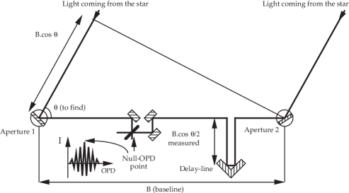
FIG. 7.: Principle of an interferometer for astrometry (Saha and Morel, 2000)

For a two-aperture interferometer (see figure 7) the external optical delay $d$, while an object with an angle $\theta$ is observed in a broad spectral range (i.e. white light), is:

$$d=|{\bf B}|\times\cos\theta.$$ (114)

This delay can be determined from the position of the optical delay-line of the instrument set up such that the central fringe of the interference pattern appears in a narrow observation window. The position, as well as $|{\bf B}|$, are measured by laser metrology. Hence, $\theta$ is deduced with a high precision. For ground-based interferometers, the baseline is fixed to the Earth and will rotate with the Earth, while in space the interferometer must reorient the baseline to measure both angular coordinates. For a space-borne interferometer, the issue is to find a reference for the angle measured. Usually, a grid of far objects like quasars are used as a reference frame. There are two modes of observation possible: the ‘wide-angle’ and the ‘narrow-angle’ modes. In wide-angle mode, the large angle difference between the reference and the studied object usually requires collector motions. In narrow-angle, the two objects are in the field of view of the instrument, therefore, no motions are required and the accuracy of the measurement is improved. However, it is difficult to have always a correct reference star within the field of view for any studied object. Narrow-angle astrometry is, therefore, more suitable for wobble characterization.

3 Nulling interferometry

Nulling interferometry was first proposed by Bracewell (1978) for applications in radio astronomy. Such an interferometer could be employed at the upcoming large interferometers to observe faint structures close to non-obscured central sources. This technique can also be used in space to search for extra-solar Earth-like planets through their thermal emission and to determine the atmospheric signature of life with spectroscopic analysis (Angel et al. 1986, Hinz et al. 1998). Here the light collected by two apertures is combined to generate a deep destructive interference fringe at the stellar position, thus selectively nulling the star by many orders of magnitude related to the surrounding off-axis environs, such as a planetary system. Basically, a $\pi$ phase-shift is introduced in one wavefront segment, so that when it interferes with another segment of the same wavefront and perfect cancellation is achieved. Therefore, the central fringe of the interference pattern is dark, allowing the fringe pattern from a faint object to appear. Unlike a coronagraph, where useful imaging is possible beyond several Airy radii from the on-axis stellar source, this method is expected to be effective within the core of a telescope’s PSF, and so can be employed for stars at greater distances, where a larger sample is available (Serabyn, 2000). The quality of a nulling is defined by the ‘null depth’ $N_{d}$:

$$N_{d}=(1-{\cal V}\cos\varphi_{e})/2\approx(\pi\sigma_{\rm\Delta\psi}/\lambda)^{2},$$ (115)

where $\varphi_{e}$ is the phase error between the two recombined beams, ${\cal V}$ the fringe visibility modulus, and $\sigma_{\rm\Delta\psi}$ the standard deviation of the optical path difference (OPD) between the two beams.

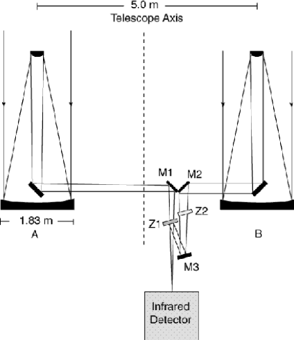
FIG. 8.: Schematic of the nulling interferometer at the MMT (Hinz et al. 1998: Courtesy: P. M. Hinz). The wavefronts from the two co-mounted telescopes A and B are translated via three mirrors M1, M2, M3 for superposition without relative rotation or tilt. The zinc selenide beamsplitters Z1, Z2 are used to adjust the path length.

To create the $\pi$ phase-shift, a few important techniques, such as (i) using roof reflectors to achieve a reversal of sign of the electric vector and (ii) introducing a precise thickness of glass whose index acts to retard all wavelengths by very nearly one-half wavelength may be used. Serabyn (2000) reported satisfactory nulling results obtained with fiber-coupled rotational shearing interferometer in visible wavelength. Hinz et al. (1998) have demonstrated the viability of nulling interferometry using two 1.8 m mirrors of the original six-mirror MMT. They have detected the thermal image of the surrounding, circumstellar dust nebula around $\alpha$ Ori. Hinz et al. (2001) have measured the spatial extent of the mid-IR emission for a few Herbig Ae stars as well. Figure 8 depicts the schematic of nulling interferometer at the MMT (Hinz et al. 1998).

B Fundamental limitations and technical challenges

Atmospheric seeing affects the measurements of fringe visibility by introducing phase aberrations across the wavefronts incident on the interferometer, the relative phase of the wavefronts at the apertures changes with time, and also varies the optical paths through the arms. Fringes are to be obtained in a time as short as atmospheric fluctuations ($\sim$0.01 s). The optical interferometers require accurate alignments, high stability, full control of any effect decreasing visibility. These limitations come from the parameters, viz., (i) precise determination of visibility, (ii) sensitivity in measuring weak sources, (iii) accurate measurement of fringe phases, and (iv) availability of range of baselines.

1 Signal-to-noise (S/N) ratio

The S/N ratio with which the visibility can be measured is a function of $N_{p}^{\prime}{\cal V}^{2}$. The fringe S/N ratio is given by the expression (Lawson, 1995),

$${\rm SNR}\propto{N_{p}^{\prime}{\cal V}^{2}\over\sqrt{1+0.5\times N_{p}^{\prime}{\cal V}^{2}}},$$ (116)

where $N_{p}^{\prime}$ is the number of photons detected per sub-aperture per integration time.

The dependence on $N_{p}^{\prime}{\cal V}^{2}$ implies that interferometry becomes increasingly difficult for faint sources, particularly for those with complex structures. The $N_{p}^{\prime}{\cal V}^{2}$ limit can be addressed in various ways, viz., (i) using larger sub-apertures, (ii) slicing of the image at the entrance of the spectrograph, (iii) bootstrapping, and (iv) tracking fringes on a point source to increase integration time on the target.

2 Delay-lines

The real art of developing interferometers is to combine the beams in phase with each other after they have traversed exactly the same optical path from the source through each telescopes down to the beam combination point. The pathlengths of the two arms need to be equalized and maintained to a fraction of $c/{\Delta\nu}$. A correct determination of ${\bf B}$ that is unstable over time is also necessary; the situation becomes complicated in the presence of atmosphere. The paths are made equal by adjusting the position of mirrors in the optical delay-line that corrects the drift induced by the diurnal rotation of the tracked star. Of course, the difficulty comes from avoiding various aberrations and vignetting, particularly when light is fed through long and narrow pipes. The optical delay in terms of telescope and source parameters translates into;

$$d = {\rm B}^{\prime}_{EW}\cos\delta_{\ast}sinH$$ (118)

$$-{\rm B}^{\prime}_{NS}(\sin\theta_{l}\cos H\cos\delta_{\ast}-cos\theta_{l}\sin\delta_{\ast}).$$

Until recently, the beam-recombining optical devices at both I2T and Grand interféromètre à deux télescopes (GI2T; Labeyrie et al. 1986) were kept on a computer controlled motor driven carriage parallel to the baseline in order to compensate the OPD. Of late, a delay-line that is movable is inserted in one of the arms of the I2T, by means of a cat’s eye system; the other arm was equipped with a fixed delay-line (Robbe et al. 1997). The present recombiner, recombineur pour grand interféromètre (REGAIN) at GI2T also uses a delay-line featuring a cat’s eye reflector with variable curvature mirror.

A few interferometers, viz., Mark III stellar interferometer (Shao et al. 1988), US Navy prototype optical interferometer (NPOI; Armstrong et al. 1998), Infrared Optical Telescope Array (IOTA; Carleton et al. 1994) use the vacuum delay-lines. Mark III interferometer delay lines used laser interferometers to measure the position of the delay line carts and nested servo loops for fine control of the OPD. Delay-lines of IOTA, have a 28 m travel ‘long’ delay-line which is moved each time a new object is observed, when the OPD to compensate is very different. It does not move during fringe acquisition. IOTA has a second ‘short’ delay-line of about 2 m travel which tracks the sidereal motion during fringe acquisition. Both the delay-lines use a dihedral (two plane mirrors at 90${}^{\circ})$ mounted on a carriage. For the long delay-line, the carriage is moved by a pulley-and-cable system powered by a stepper motor, while for the short delay-line a linear motor system allows precise motion of the carriage (10 nm steps). For both delay-lines, measurement of the carriage position is done by a laser metrology system using the Doppler-Fizeau effect of a laser beam sent to the carriage and bouncing back (Morel, 2000).

Another method known as group-delay tracking, based on the integration of the moduli of all the computed FTs (Lawson, 1994, Lawson et al. 1998), is used with the interferometers SUSI, and COAST. The group-delay is proportional to the rate of change of phase as a function of wavenumber, evaluated at the center of the band. This delay can be measured if the combined beams from an interferometer are dispersed in a spectrometer. The group-delay tracking yields a peak whose position is proportional to the OPD.

3 Beam recombination

Fringes can be obtained either by utilizing the concept of merging speckles (Labeyrie, 1975) or by employing pupil-plane configuration (Tango and Twiss, 1980). At the initial stage, the beam recombining optics that were employed at both I2T and GI2T consisted of (i) a recombining element for reconfiguring the pupil and fixing the fringe spacing, (ii) an image slicer (a series of 10 wedges of different angles cemented on a field lens slices the image), (iii) the compensating system of the atmospheric dispersion, (iv) gratings (maximum spectral resolution 0.15 nm), and (v) detectors to record the fringes. The advantages of the dispersion mode are the capabilities (i) of allowing continuous observation of fringes across the spectral bandwidth, (ii) of recording the fringes with longer integration time, and (iii) of selecting different spectral channels for differential visibility measurements. In the REGAIN combiner, each coudé beam coming from the telescopes meets a pupil stabilizer, a field rotator, a wedge prism and the beam combiner (Rousselet-Perraut et al. 1996). Figure 9 depicts the process performed by an arm of the REGAIN table prior to recombination.

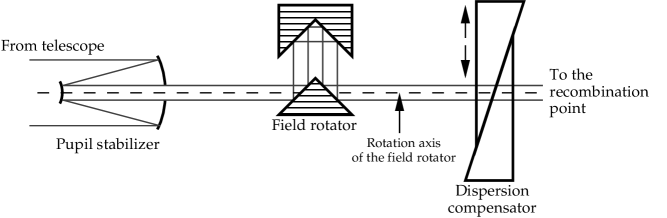
FIG. 9.: Optical processing of a beam from one arm of GI2T by the REGAIN recombiner (Saha and Morel, 2000).

Interferometry with multiple apertures, such as COAST uses multi-stage four-way combiner. Light from the telescopes is first combined in pairs. These pairs are recombined with other pairs. Each detector sees light from all of the telescopes. Another method known as pair-wise recombination technique is employed at NPOI, where a beam combiner uses a different detector for each baseline.

a Fiber-linked recombination

Fiber optics systems provide a perfect spatial filtering of the turbulence-induced corrugated wavefronts and find that the contribution variations are much reduced. The advantages of this may be envisaged in the form of (i) selecting the plane-wave part of a wavefront, (ii) splitting a guided wave into any desired intensity ratio, and (iii) combining two guided waves interferometrically. The significance of the fiber-linked unit for optical recombination (FLUOR), IOTA is that visibilities can be calibrated with sub-1% precision, which is important for many astrophysical applications like stellar atmospheres studies, Cepheid pulsation measurements for distance determinations, and detection of angular anisotropies arising in disks around young stars.

The fiber delay-lines, using spools of fiber that can be stretched or relaxed to increase or decrease the optical pathlength are used in FLUOR. These fibers have been designed to propagate infrared light at near-IR (Mennesson et al. (1999) in TEM mode, like a coaxial cable. Therefore, only plane-waves perpendicular to the axis of the fiber may propagate over long distance. Basically, this method results in a ‘spatial filtering’, thus smoothing the wavefront. The advantage of such a method for interferometry is a reduction of the uncertainty on the measured visibility, and the drawbacks are the loss of optical coupling efficiency and larger photometric variations due to the turbulence. Figure 10 depicts the schematic of the FLUOR recombiner.

FIG. 10.: Schematic of the FLUOR recombiner. ${\tt P}1$ and ${\tt P}2$ are the photometric output fibers. ${\tt I}1$ and ${\tt I}2$ the interferometric output fibers. These outputs are imaged by a lens on a NICMOS infrared array detector (Saha and Morel, 2000).

b Integrated optics

The integrated optics (IO), analogous to integrated chips in micro-electronics, potentially allows large tables of bulk optics to be replaced by miniature devices (Haguenauer et al. 2000). Such hardware provides easy access to spatial filtering and photometric calibration. The astronomical validation of this approach to interferometrically combine beams from separated telescopes at IOTA has been reported recently by Berger et al. (2001). Two different chips designed for two-telescope beam combination in H band were used by them. One is manufactured using the ion exchange process: Na⁺ ions from a glass substrate are exchanged with Ag⁺ ions in a molten salt through a dedicated mask and the other is manufactured using silica etching technique.

c Polarization

For phased combination either in the image-plane or in the pupil-plane, the individual incoming beams from the arms of an interferometer should have identical pupil orientations, image orientations, and polarization characteristics (Traub, 2000). If the corresponding mirrors at each reflection (in the case of two telescope interferometer) are of same type, both the beams will experience the same phase-shifts; the respective $s$ and $p$ components combine independently in the focal-plane and produce identical fringe packets. If the sequence of reflections is different, the visibility ${\cal V}_{pol}$, of an interferogram is,

$${\cal V}_{pol}=|cos\frac{\psi_{sp}}{2}|,$$ (119)

where $\psi_{sp}$ is the $s-p$ shift between the two beams. The loss of coherence due to misalignment of optical train, aging of coatings, and accumulation of dust can also be analyzed (Elias, 2001).

At GI2T, the REGAIN uses the field rotators consisting of four plane mirrors for each beam to compensate the polarization difference. In the COAST, starlight passing through the central siderostat undergoes an additional two reflections so that its $s$ and $p$ polarizations experience the same reflections as light from the other siderostats (Baldwin et al. 1998).

Fibers have a natural birefringence that introduce elliptic polarization at the output, when linearly-polarized light is injected which causes a loss of the measured visibility. A solution for compensating the fiber birefringence consists in winding the fibers into one or two loops (Lefèvre 1980). The supplementary birefringence introduced by this system depends on the radius of the loops; it cancels the effects of the natural birefringence. With this system, the polarization plane can be rotated by twisting the fiber (by displacing the loops around the main fiber axis). Another solution to minimize birefringence effects consists in using a Babinet compensator (a birefringent quartz crystal consisting of two thin prisms cemented together to form a thin parallel plate) at the input of each fiber.

d Dispersion

A compensating system for correcting atmospherically induced dispersion is essential at the recombiner. In the REGAIN, the different ‘chromatic dispersions’ between the two beams are compensated by using two prisms which can slide on their hypotenuse, forming therefore, a plate with adjustable thickness. This thickness is modified every 4 minutes, following the variation of the altitude of the observed object (Rousselet-Perraut et al. 1996).

In the case of fiber-linked recombiner, the dispersion of a fiber optics coupler made by two fibers of 1 and 2 is expressed by the phase curvature:

$$\frac{{\it d}^{2}\psi}{{\it d}k^{2}},$$ (120)

where $\psi$ is the phase of the spectrum of the interferogram. It is demonstrated by Coudé du Foresto et al. (1995) that the phase curvature can be given by:

$$\frac{{\it d}^{2}\psi}{{\it d}k^{2}}=-2\pi c\lambda^{2}(\nabla_{2}\Delta L+L_{1}\Delta\nabla),$$ (121)

where $\nabla_{2}$ is the dispersion coefficient of fiber 2, $\Delta L=L_{2}-L_{1}$ the difference of length between the two fibers, and $\Delta\nabla=\nabla_{2}-\nabla_{1}$ the difference of dispersion. The dispersion coefficient depends on the refractive indexes of both the core and the cladding of the fiber. One problem of fiber dispersion is the ‘flattening’ of the interferogram, reducing the fringe contrast. To minimize the dispersion, the length of each fiber must be calculated from the dispersion coefficients of each fiber.

4 Calibration

Due to the atmospheric turbulence affecting the wavefronts before recombination, measurements of ${\cal V}$ are biased by a random factor depending on the seeing quality. Instrumental flaws leading to optical aberrations and non-balanced flux between the two beams modify the measured visibility modulus as well. It is, therefore, important to calibrate each measure on an object by measuring ${\cal V}$ on an non-variable unresolved source (e.g., a farther star) in the neighborhood, preferably within 1^∘ of the program star to minimize motions of telescopes and delay-lines, and at the same turbulence condition. The calibrator and the studied object observations should be interleaved for recording the fringes on both back and forth a few times during the observing run. Hence, one can interpolate the transfer function for each object-observation period. To reproduce the instrumental conditions, the calibrator must roughly be as bright as the object to calibrate; it should have ideally a spectral type and a magnitude similar to the studied object. The calibration of the resulting visibility is given by, ${\cal V}_{cal}^{2}={\cal V}^{2}/{\cal V}^{2}_{ref}$ (Berio, Mourard et al. 1999).

5 Fringe-tracking

Fringes are searched by adjusting the delay-line position; however, mechanical constraints on the instrument, errors on the pointing model, thermal drifts, various vibrations and atmospheric turbulence make the null-OPD point changing. The error on the OPD must be less than the coherence length defined by:

$$l_{c}=c\cdot\tau_{c}={\bar{\lambda}^{2}\over\Delta\lambda},$$ (122)

where $\bar{\lambda}$ is the mean wavelength observed and $\Delta\lambda$ is the spectral interval. This real-time control is called ‘fringe-tracking’.

There exist three possible set-ups for fringe acquisition for visible spectrum. In the first one, the OPD is temporally modulated by a sawtooth signal, using a fast and short-travel delaying device. The intensity of the recombined beams, describes therefore, over the time a fringe pattern that is recorded by single pixel detectors. The second method consists of imaging the dispersed recombined beam on a linear detector. In the third one, beams are dispersed prior to the recombination; recombination is done by focusing them with a common lens like in Michelson stellar interferometer. In IR, it is essential to use as little pixel as possible in order to reduce global readout noise. The ‘white’ fringes set-up is preferably used for IR observations.

a Coherencing and cophasing

Techniques to compensate the OPD drift between the two beams of a standard optical interferometer may be classified into two categories: coherencing and cophasing. The aim of the former is to keep the OPD within the coherence area of the fringes, while the latter, the OPD must remain much smaller than the wavelength: fast compensation of the OPD variations due to the differential ‘piston’ mode of the turbulence is, therefore, done in order to ‘freeze’ the fringes.

The coherencing with non-white fringes is compared with the active optics. In white light it is done, as for IOTA, by scanning the OPD while acquiring signals to find the null-OPD point in the fringe pattern (Morel et al. 2000). This coherencing yields the OPD correction to apply to the delay-line, at a few Hz servo-loop rate. With a channeled spectrum, the OPD is proportional to the fringe frequency. Another method, viz., the real time active fringe-tracking (RAFT) system has been applied to dispersed fringes on GI2T using 2-d FT (Koechlin et al. 1996). Both group-delay tracking and RAFT allow a slow servo-loop period (up to a few seconds) by multiplying the coherence length by the number of spectral channels used.

Cophasing that may be compared with the AO system, is performed with white fringes, using the synchronous detection method; the OPD is quickly scanned over a wavelength range. The signal acquired from the detector is then processed in order to yield the phase-shift and the visibility, which can be done by integrating signal (Shao and Staelin, 1977) over four $\lambda/4$ bins, named $A$, $B$, $C$ and $D$. Phase-shift and visibility modulus are then given by,

$$\Delta\varphi = \arctan\left({B-D\over A-C}\right)$$ (123)

$${\cal V} = {\pi\sqrt{(A-C)^{2}+(B-D)^{2}}\over\sqrt{2}(A+B+C+D)}.$$ (124)

Fringe-tracking methods may be enhanced by introduction of a priori information, in order to allow observations at fainter ${\cal V}$ or fainter magnitudes. Gorham (1998) has proposed to improve white light cophasing by filtering data with a function computed to reduce the photon noise. The gain for the tracking limit magnitude, at constant ${\cal V}$, is between 0.5 and 0.7. Methods introducing a priori information for GDT or RAFT have been imagined as well (Padilla et al. 1998, Morel and Koechlin, 1998).

b Bootstrapping

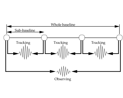
FIG. 11.: Principle of baseline bootstrapping. Apertures are represented by circles (Saha and Morel, 2000).

It is possible to stabilize the fringes using bootstrapping methods at the interferometers. These methods can be categorized into two systems, namely, wavelength bootstrapping and baseline bootstrapping. It may be optimal to employ the former that requires two recombiners, one for visibility measurement, the other one for fringe-tracking. For example, at long baselines, when the expected fringe visibility is too low for tracking, it is possible to use a longer wavelength where the fringe contrast, for a white object, is higher. Meanwhile, fringes for computing the visibility are acquired at shorter wavelength than for tracking. This method was applied at Mark III interferometer (Quirrenbach et al. 1996). On the other hand, the latter is performed by tracking fringes over a connected series of short baselines to allow low visibility fringes to be measured on the longest baseline. In this method the photons are shared and it works well because of the closure-phase relationships. Here the baseline is divided into sub-baselines by adding apertures along the baseline. Fringe-tracking is performed on each sub-baseline, where the visibility is higher than with the entire baseline. Hence, fringes are tracked on the whole baseline as well. Figure 11 depicts the principle of baseline bootstrapping. NPOI employs such a system that enables one to reach spatial frequencies beyond the first visibility null (Pauls et al. 1998). A related idea has been developed for the Keck interferometer, as well as for the ESO’s very large telescope interferometer (VLTI).

c Role of AO systems

An interferometer works well if the wavefronts from the individual telescopes are coherent. The maximum useful aperture area is proportional to $\lambda^{12/5}$. In order to improve the sensitivity of an interferometer where it is used to target faint sources, each telescope will have to be reasonably large. A large aperture produces more than 100 speckles in the image and the fringe pattern within each speckle is randomly phased. Enough photons are required to phase the telescopes into a coherent aperture, therefore, to enhance the instrumental visibility, an AO system should be incorporated. A typical image-width reduction of roughly a factor of 10 and a central intensity enhancement of a factor of 10^1.5 can be achieved on large telescopes (Traub, 2000). Though complete AO systems have not been implemented at any of the interferometers to date, baring Keck-I which uses full-AO corrections, a few of them, viz., GI2T, IOTA are using tip-tilt control system. This correction is sensed in the visible, using CCDs, and fringe detection is done in the near-IR. IOTA tip-tilt correction system uses a 32$\times$32 pixel CCD for each beam. The maximum rate is 200 Hz (Morel, 2000). A computer reads each frame and computes the centroid. The value of the centroid position is sent to a piezo mirror placed downstream the secondary mirror of each telescope.

C Data processing

The optimal integration time required for measuring a visibility point is a trade-off between the number of photons to collect and the Earth rotation shifting the sampled point in the $(u,v)$ plane. Though with the large Binocular Telescope (LBT), the two 8.4 m mirrors will be installed on a common alt-az mounting, thus information in the $u,v$ plane can be continuously combined or coadded, most of the interferometers use two apertures and are unable to recover the complex visibility. Therefore, the information to extract from a batch of fringes is the modulus of the visibility. Theoretically, using merely the Fourier transform would give an optimal estimate of the visibility modulus, as demonstrated by Walkup and Goodman (1973). However, white-light fringes obtained from coherencing are flawed by the differential piston that modulates their frequency. Techniques used in radio-interferometry (where wavelengths are much longer), like fitting a sinewave through the fringe data, are therefore, not suitable. Perrin (1997) has proposed a method to remove the piston from fringes. However, this method requires a high fringe SNR ratio and may only be applied when fringe SNR is important.

1 Recovery of visibility functions

The model visibility amplitude ${\cal V}(s_{\lambda})$ for a uniform source of diameter $\phi_{UD}$ is given by,

$${\cal V}(s_{\lambda})=\pm\frac{1}{{\sl F}_{0}}\int_{-\phi_{UD}/2}^{\phi_{UD}/2}{\sl B}(\theta)cos[2\pi s_{\lambda}\theta]d\theta,$$ (125)

where ${\sl F}_{0}$ and ${\sl B}(\theta)$ are the respective total flux and the brightness distribution of the source, $\theta$ the position angle of the source and $s_{\lambda}$ the baseline length in wavelengths. This equation reduces to,

$${\cal V}(s_{\lambda})=\frac{sin[\pi s_{\lambda}\phi_{UD}]}{\pi s_{\lambda}\phi_{UD}}$$ (126)

For the objects with circular symmetry, the visibility function is expressed as,

$${\cal V}(s_{\lambda})=\biggl{|}\frac{2J_{1}(\pi s_{\lambda}\phi_{UD})}{\pi s_{\lambda}\phi_{UD}}\biggr{|},$$ (127)

where $J_{1}(\pi s_{\lambda}\phi_{UD})$ is a Bessel function of the first kind. However, a problem arises due to the limb-darkening of the stars. Observations of limb darkening measurements require one to collect data in the vicinity of and beyond the first zero or minimum of the visibility function. The radial intensity profile of a star may be given (Hestroffer, 1997) by:

$${\cal I}(\mu)={\cal I}(0)\mu^{\alpha_{l}},$$ (128)

where ${\cal I}(\mu)$ is the disk brightness at angle $\mu(=cos\theta)$, $\theta$ the angle between the normal to the stellar surface and the direction to the observer, and $\alpha_{l}$ is the limb-darkening factor depending on the stellar atmosphere. The visibility function in this case may be derived as,

$${\cal V}(s_{\lambda})=\Gamma({\it n}+1)\frac{|2J_{\it n}(\pi s_{\lambda}\phi_{LD})|}{(\pi s_{\lambda}\phi_{LD}/2)^{\it n}},$$ (129)

where ${\it n}=(\alpha_{l}+2)/2$ and $\phi_{LD}$ is the limb-darkened diameter of the source. Many interferometers cannot measure low visibilities existing at high angular frequency (i.e, when $\sqrt{u^{2}+v^{2}}$ is large), beyond the first minimum of the visibility function. Reconstructions are, therefore, ambiguous and neither the diameter nor the limb-darkening factor may be accurately determined. Usually, $\alpha_{l}$ is an a priori information given by the stellar atmosphere model. The diameter is, therefore, deduced from $\alpha_{l}$ and the interferometric data. Figure 12 represents two visibility curves of the Mira type variable star R Leo, obtained by the FLUOR/IOTA combination in the K band at two different epochs, which show both the change in equivalent UD disk diameter and (for the 1997 data) the diffusion by circumstellar material whose signature is a visibility curve substantially different from that of a uniform disk (Perrin et al. 1999).

FIG. 12.: Visibility curves of the Mira variable R Leo (Courtesy: V. Coudé du Foresto).

For two unresolved sources, e.g., a binary system, the expression is formulated to,

$${\cal O}({\bf x})={\sl B}_{1}\delta({\bf x}+{\bf x}_{0})+{\sl B}_{2}\delta({\bf x}+{\bf x}_{0}+{\bf x}_{s}),$$ (130)

where $|{\bf x}_{s}|$ is the angular separation between two sources and ${\sl B}_{1}$, ${\sl B}_{2}$ the brightnesses of the source 1 and source 2, respectively. The visibility modulus corresponding to this function at ${\bf u}$ is, therefore:

$$|\widehat{\cal O}({\bf u})|=\sqrt{({\sl B}_{1}-{\sl B}_{2})^{2}+4{\sl B}_{1}{\sl B}_{2}\cos^{2}(2\pi{\bf u}.{\bf x}_{s})}.$$ (131)

It is then useful to use a technique called ‘super-synthesis’: the $(u,v)$ plane is swept during an observation lasting several hours, due to Earth rotation. After a large variation of hour angle $H$, several visibility moduli are, therefore, measured at different $(u,v)$ points to determine the parameters (${\sl B}_{1}$, ${\sl B}_{2}$ and ${\bf x}_{s}$) of the system by fitting the function described by the equation (117).

The visibility function of the thin structures of the circumstellar shell may be computed by considering a coaxial uniform disk and a point source; therefore, the function is written as,

$${\cal V}(s_{\lambda})=V_{p}+(1-V_{p})\biggl{|}\frac{2J_{1}(\pi s_{\lambda}\phi_{s})}{\pi s_{\lambda}\phi_{s}}\biggr{|},$$ (132)

where $\phi_{s}$ is the diameter of the shell and $V_{p}$ the ratio of power radiated by the star.

2 Derivation of effective temperatures

Combining photometry with the measurement of limb-darkened stellar diameter yield the stellar emergent flux, ${\sl F}_{e}$ or surface brightness and is found from the relation,

$${\sl F}_{e}=\frac{4{\sl F}_{\nu}}{\phi_{LD}^{2}},$$ (133)

where ${\sl F}_{\nu}$ is the measured absolute monochromatic flux received from the star at frequency $\nu$.

The stellar effective temperature $T_{e}$ is defined in terms of the emergent flux by the Stefan-Boltzmann law. Integrating over all frequencies,

$${\sl F_{e}}=\int{\sl F}_{\nu}d\nu=\sigma T_{e}^{4}$$ (134)

where $\sigma$ is Stefan constant.

D Ground-based optical/IR arrays

Several ground-based LBOIs have been developed to obtain very high angular resolution informations of the stellar objects. However, three of them, viz., (i) I2T (Labeyrie, 1975), Plateau de Calern, France, (ii) Mark III interferometer (Shao et al., 1988), Mt. Wilson, USA, and (iii) Infrared interferometer, SOIRDÉTÉ (Gay and Mekarnia, 1988), Plateau de Calern, France are no longer in operation.

1 Direct detection interferometers

I. Labeyrie et al. (1986) have developed GI2T interferometer with two ‘boule’ telescopes that run on North-South tracks with variable baseline of 12 to 65 m. This instrument at Plateau de Calern, France combines the features of the Michelson design and the radio interferometers; it operates in speckle mode. It consists of a pair of 1.52 m telescopes on altitude-altitude mounts. Each telescope is housed in a sphere (3.5 m diameter) made of concrete, which has three mirrors directing the horizontal afocal coudé beam to the recombiner optics. Light beams from both the telescopes are superposed at the foci in order to produce Young’s fringes. The driving system of the sphere consists of a pair of rings; each ring is motorized by 3 actuators acting in 3 orthogonal directions within 2 different tangential planes. The two rings alternately carry the sphere, which in turn, produce continuous motion with a resolution of the order of 1 $\mu$m. The main drawback comes from the slow pointing of the telescopes; 4 or 5 stars can be tracked during the night.

II. The SUSI, Sydney University, Australia has a very long baseline ranging from 5 m to 640 m (North-South) that are achieved with an array of 11 input stations equipped with a siderostat and relay optics, located to give a minimal baseline redundancy (Davis et al. 1999a); the intermediate baseline forms a geometric progression increasing in steps of $\sim$40%. Starlight is steered by two siderostats of 20 cm diameter into the evacuated pipe system that carries the light to the atmospheric refraction corrector (at the central laboratory) consisting of the pairs of counter-rotating Risley prisms via a beam reducer. It proceeds towards either the optical path length compensator (OPLC) or is diverted towards the acquisition camera. On leaving OPLC, the beams from the two arms of this interferometer may be switched over to one of the optical tables (blue or red) for recombination.

III. The COAST, Cambridge, UK uses four independent telescopes consisting of 50 cm siderostat flat feeding a fixed horizontal 40 cm Cassegrain telescope with a magnification of 16. These are arranged in a Y-layout with one telescope on each arm, movable to a number of fixed stations and one telescope at the center of the Y (Baldwin et al. 1998). Light from each siderostat passes through pipes containing air at ambient pressure into the beam combining laboratory (inside a tunnel). The four beams emerging from the path compensator are each split at a dichroic; the longer wavelength ($\lambda>$650 nm) of the visible band passes into the beam combining optics and the shorter ones are used for acquisition and autoguiding. Each output beam passes through an iris diaphragm and is focused by a long focus lens on to a fiber fed single-element avalanche photodiode detector for fringe detection.

IV. The IOTA, situated at Mt. Hopkins, Arizona consists of three 45 cm collector assembly located at various stations on the L-shaped baseline (5-38 m) that comprises a siderostat, an afocal Cassegrain telescope and an active relay mirror (Traub et al. 2000). In the recombining table, the optical differences are compensated by fixed and variable delays and the beams are recombined onto a beam splitter, producing two complementary interference signals (Carleton et al. 1994). A fast autoguiding system is used to correct the atmospheric wavefront tilt errors. Two active delay-lines for three telescopes are provided; a scanning piezo mirror is used to modulate the OPD between the two telescopes.

V. The NPOI, located at Lowell Observatory, Arizona, is designed to measure positions with precision comparable to that of Hipparcos (1997). However, the aperture sizes limit the array to bright star astrometry. It is developed as Y-shaped baseline configuration that includes sub-arrays for imaging, and for astrometry. For the astrometric mode, four fixed siderostats (0.4 m diameter) are used with the baselines extendable from 19 m to 38 m. The astrometric sub-array has a laser metrology system to measure the motions of the siderostats with respect to one another and to the bedrock. While for the imaging mode, 6 transportable siderostats (0.12 m diameter) are used. Three siderostat positions are kept with equal space for each arm of the Y. Coherence of imaging configuration is maintained by phase bootstrapping. The synchronous detection method applied to signals from several spectral channels, has been used as well (Benson et al. 1998).

VI. The Palomar testbed interferometer (PTI), Palomar Observatory, California is an IR phase-tracking interferometer that was developed as a test-bench for the Keck interferometer. The main thrust is to develop techniques and methodologies for doing narrow angle astrometry; therefore, it is designed to observe two stars simultaneously to measure the angle between them with high precision. It uses coherent fringe demodulation and active fringe-tracking systems with an array detector at 2.2 $\mu$m and active delay-lines with a range of $\pm$38 m. It is comprised of three 40 cm siderostats that are coupled to beam compressors. These siderostats are used pairwise to provide baselines up to 110 m (Colavita et al. 1999). Both phase and group-delay measurements for narrow angle astrometry are being carried out (Lawson et al. 2000). Visibility is estimated from the fringe quadrature, either incoherently, or using source phase referencing to provide longer integration time (Colavita, 1999).

2 Heterodyne interferometry

Heterodyne technique is generally used in radio-astronomy to reduce the high frequency signal to an intermediate one. Such a technique has the following advantages in the case of beam recombination in IR interferometry. They are: a larger coherence length, a simplification of the transport of the signal from the collector to the recombiner (coaxial cables instead of mirrors). Let ${\cal U}_{\it s}(t)$ and ${\cal U}_{\it l}(t)$, be respectively the signals of a wave coming from a star and of an artificial source (laser), which are expressed as,

$${\cal U}_{\it s}(t) = {\it a}_{\it s0}.e^{-i[\omega_{\it s}.t-\psi]},$$ (135)

$${\cal U}_{\it l}(t) = a_{\it l0}.e^{-i\omega_{\it l}.t}.$$ (136)

The laser is the phase reference. A detector like a photodiode, illuminated by the sources (star + laser) yields an electrical signal corresponding to the light intensity:

$${\cal I}(t) = |{\cal U}_{\it s}(t)+{\cal U}_{\it l}(t)|^{2}$$ (140)

$$=({\it a}_{\it s0}.e^{-i[\omega_{\it s}.t-\psi]}+{\it a}_{\it l0}.e^{-i\omega_{\it l}.t})$$

$$\times({\it a}_{\it s0}.e^{i[\omega_{\it s}.t+\psi]}+{\it a}_{\it l0}.e^{-i\omega_{\it l}.t})$$

$$={\it a}_{\it s0}^{2}+{\it a}_{\it l0}^{2}+2.{\it a}_{\it l0}.{\it a}_{\it s0}.\cos[(\omega_{l}-\omega_{s})+\psi].$$

If $\omega_{\it l}$ and $\omega_{\it s}$ are close, the frequency of ${\cal I}$ is low enough to fit in the bandwidth of the detector and its electronics (a few GHz) and ${\cal I}$ carries the phase information from the radiation of the star. By correlating (multiplying) the signals ${\cal I}_{1}$ and ${\cal I}_{2}$ yielded by two apertures with heterodyning systems, one can extract a visibility term. However, the lasers must have the same phases for the two apertures.

The heterodyne interferometry at 8-11.5 $\mu$m spectral range was employed on the SOIRDÉTÉ, Observatoire de Calern, France, an IR interferometer that consisted of a pair of 1 m telescopes with a 15 m East-West horizontal baseline (Gay and Mekarnia, 1988). It was an interesting project but ultimately a failure and produced no significant scientific results. In this project, beams were received in the central laboratory on a double cat’s eye delay-line on a step by step movable carriage; natural OPD drift due to the Earth-rotation was used for acquiring fringes (Rabbia et al. 1990). Heterodyne interferometry is also used on the recently developed mid-IR spatial interferometer (ISI), Mt. Wilson, California (Townes et al. 1998), which is an outstanding success with many scientific results. It is well suited to study of circumstellar material around bright evolved stars. It features three movable telescopes; each telescope comprises a 1.65 m parabolic mirror and a 2 m flat mirror equipped with an automated guiding and tip-tilt control system at 2 $\mu$m (Lipman et al. 1998). The star light from each aperture is first mixed with a stable ${\rm CO}_{2}$ laser local oscillator, converting the signal to microwave frequencies, followed by pathlength matching and fringe detection in a correlator. On ISI, two ${\rm CO}_{2}$ lasers are used, the phase of one being controlled by the other. Here the interferometer noise is dominated by shotnoise of the laser and thermal background is negligible for setting the sensitivity limit (Hale et al. 2000). ISI utilizes Earth rotation and periodic discrete changes of the baseline to obtain a wide range of effective baselines and map the visibility functions of the stellar objects.

E Projects under development and planned

I. The Center for High Angular Resolution Astronomy (CHARA) array at Mt Wilson, California comprises six fixed 1 m telescopes arranged in a Y-shaped configuration with a maximum baseline of $\sim$350 m that will operate at optical and IR wavelengths (McAlister et al. 1998) with a limiting resolution of 0.2 mas. The key scientific goal of this interferometer is binary star astrometry, observations of stars with well-determined spectroscopic elements, and determination of the metal abundance.

II. The Mitaka optical-IR array, National Astronomical Observatory, Japan consists of several interferometers built one-by-one. The first of the series was MIRA-I (Machida et al. 1998) that has 25 cm siderostats and a 4 m baseline. Its successor, MIRA-I.2 (Sato et al. 1998) has the same baseline and slightly larger siderostats (30 cm). It features equipment encountered on many operating interferometers: beam compressors (yielding 30 mm beams), delay-line operating in vacuum, tip-tilt correction system and laser metrology. These instruments are specially designed for astrometry.

III. The large binocular telescope (LBT), on Mt. Graham, Arizona that consists of two 8.4 m primary mirrors (Hill, 2000) is under construction, The LBT mirrors are co-mounted on a fully steerable alt-az mounting, in which variable delay lines for the path equalization are not needed. At near-IR wavelengths, a field of view of one arcminute or more is expected with unprecedented spatial resolution of order of 8-9 mas at $\lambda\sim 1~{}\mu$m and a variable baseline of 0-23 m (Wehinger, 2001).

Another interferometer, the Magdalene Ridge observatory array, USA with three element (2$\times$2.4 m plus 0.8 m) has also received initial funding and is under development.

1 Interferometers of heterogenous nature

The Keck interferometer, Mauna Kea, USA (Colavita et al. 1998), and (ii) VLTI, ESO, at Paranal, Chile (Derie et al. 2000) are of a heterogenous nature. The problem comes from the recombination of two telescopes, one large and one small because the S/N ratio would be the one given by the small telescopes. Nevertheless, the recent success of obtaining interferometric fringes from the starlight by the two large telescopes at both Keck (http://www.jpl.nasa.gov/news) and VLTI (Glindemann and Paresce, 2001) will have an enormous impact on developing future large optical arrays.

The Keck interferometer comprises of two 10 m and four 1.8 m ‘outrigger’ telescopes; for imaging the main telescopes would be used with outriggers to fill in incomplete parts of the $u,v$ plane. It will combine phased pupils provided by adaptive-optics for the main telescopes and fast tip/tilt correction on the outriggers. Beam recombination will be carried out by 5 two-way combiners at 1.5-2.4 $\mu$m for fringe-tracking, astrometry, and imaging. A project for a 10 $\mu$m nulling-combiner for exo-zodiacal disk characterization is in the planning stages. A differential phase technique to aim at detecting faint sources near a bright object is also under development (Akeson et al. 2000).

While in the case of VLTI, beams are received from the movable telescopes in a central laboratory for recombination and are made to interfere after introducing suitable optical delay-lines. coudé beams from these apertures are sent through delay-lines operating in rooms at atmospheric pressure but at accurately controlled temperature. The beams reach an optical switch-yard to be directed to one of the four expected recombiners, e.g., (i) a single mode fiber recombiner (2.2 $\mu$m) that intends to debug the upstream sub-system of VLTI, (ii) a beam splitter based recombiner that operates at 10 $\mu$m, (iii) a recombiner that operates between 1 $\mu$m - 2.5 $\mu$m, and (iv) a recombiner for narrow angle astrometry.

2 Interferometry with large arrays

The next generation imaging interferometers with at least 15 or more elements should have the snapshot capability in an instantaneous mode. Beams from separated telescopes of such an interferometer must be recombined in the focal point as in the case of a Fizeau interferometer that is optically equivalent to single large telescope masked with a multi-aperture screen so as to reproduce exactly the ensemble of collecting telescopes (Traub, 1986).

Development of an optical very large array (OVLA), an array of 27 telescopes of 1.5 m diameter was initiated more than a decade ago by Labeyrie, Lamaitre et al. (1986). Each telescope is housed in a fiberglass sphere (Dejonghe et al. 1998) that is mounted on a six-legged robot to enable it to move on the ground while fringes are acquired, eliminating the need for optical delay-lines. A secondary mirror makes the beam afocal and compressed. A third steerable flat mirror sends this beam out through a slit located on the sphere to the central station where all other beams coming from other telescopes are combined into a single high resolution image. OVLA has also been considered for different possible aperture diameters including 12 to 25 m (Labeyrie, 1998). A new telescope structure has been imagined for this class of very large collectors: the ‘cage telescope’, in which the sphere is replaced with an icosahedral truss steerable by a different mechanical system. Ridgway and Roddier (2000) have proposed a project of developing IR_VLA with a total baseline of $\sim$1000 m, consisting of 27 telescopes with each aperture of 4 m. Another proposed project called ‘Large-Aperture Mirror Array’ (LAMA) employs eighteen fixed 10 m liquid-mirror telescopes located within a circle of 60 m diameter which collect 50% of the light that falls within this area (Hickson, 2001).

3 Hyper-telescope imaging

The ‘densified-pupil multi-aperture imaging interferometry’ may provide direct images at their focal-plane, albeit it is a subtle technique. Conceptually it differs from the Fizeau interferometers which become inefficient when the sub-aperture spacing is large compared to their size. The reason is that most energy goes in a broad diffractive halo rather than in a narrow interference peak, which precludes obtaining usable snapshot images with kilometric or megametric arrays in space.

Densifying the exit pupil, i.e., distorting it to increase the relative size of the sub-pupils, in such a way that the pattern of sub-aperture centers is preserved, concentrates the halo and intensifies the image (Labeyrie, 1996). Figure 13 depicts the concept of the hyper-telescope. Pedretti et al. (2000) have derived the integrated intensities of the central peaks of the images on the star Capella that are obtained by taking two separate exposures of 100 s in the Fizeau and densified-pupil mode of the hyper-telescope. The comparison of these values showed an intensity gain of 24$\pm$3$\times$ of the densified with respect to the Fizeau configuration. Imaging arrays of huge size, possibly approaching a million kilometers to observe neutron stars, may become feasible in this way, called ‘hyper-telescopes’. They provide an image with full luminosity in a narrow field of $\approx\lambda/B_{s}$, where $B_{s}$ is the distance between the sub-apertures of the array.

In practice for ground arrays, an elliptical track is one way of compensating the Earth’s rotation, but with delay lines, a periodic dilute-aperture can also be built at the scale of 10 kilometers. In space, it would be a periodic hexagonal paving in the case of hyper-telescope version proposed by Labeyrie (2001) for space interferometer, Terrestrial Planet Finder (TPF). This version has a Fizeau focus followed by a small pupil densifier, and a coronagraph (Boccaletti et al. 2000). Unlike the ground-based elliptic ring where images are directly obtained at a recombination station located at a focus of the ellipse or periodic arrays on the ground, space arrays can be globally pointed.

The cophasing of the array may be done hierarchically (Pedretti and Labeyrie, 1999) by cophasing triplets of beams (yielding a honeycomb pattern in the image-plane), then triplets of triplets, etc. Piston errors are measurable from the triplet images. Another way of analyzing the piston errors (Labeyrie, 1999a) is an extension of the classical dispersed-fringes used since Michelson: a set of monochromatic images recorded with a spectro-imager is organized as an $x,y,\lambda$ data cube, and its 3-dimensional FT is calculated to extract piston errors in pairs or triplets of apertures.

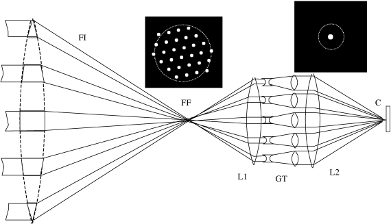
FIG. 13.: Principle of the hyper-telescope (Courtesy: A. Labeyrie). The focal image ${\tt FF}$ provided by a Fizeau interferometer ${\tt FI}$ is re-imaged by lenses ${\tt L}1$ and ${\tt L}2$ on camera ${\tt C}$, through an array of miniature and inverted Galilean telescopes ${\tt GT}$. They densify the exit beam, thus shrinking the diffractive envelope (dotted circle) of the focal pattern with respect to the interference peak. For an off-axis star, they also attenuate the local tilt of the flat wavefront transmitted from ${\tt L}1$, while preserving the global tilt. The wavefront from an off-axis star thus acquires stair steps while becoming densified at ${\tt L}2$. The interference peak is displaced more than the envelope, but remains within it if the step is below one wavelength.

F Space-borne interferometry

The advantage of deploying LBI in space is that of observing can be done at any wavelength and for longer duration in the absence of atmospheric turbulence. The difficulty comes from developing a technology featuring high precision positioning, as well as toughness required for space operation. A new generation of ultra-lightweight active mirrors (Burge et al. 2000, Angel, 2001) are essential to resolve the problems of size and weight.

1 Space technology 3

This new generation of scientific spacecraft, ST3 (Gorham et al. 1999), NASA’s mission, scheduled for 2003, consists of two independent free-flying elements launched into an Earth-trailing heliocentric orbit. One is a collector sending light from the observed object to the second element featuring another collector, an optical delay-line and a beam recombiner. The aim of ST3 is the demonstration and validation of technologies that might be used for future space-borne interferometers. Thus, the two elements of ST3 should be able to move up to 1 km from each other, while being controlled by a laser metrology. However, the designed delay-line of ST3 can be up to 20 m of optical pathlength only. This instrument will be used as an imaging interferometer for studying such objects as Wolf-Rayet or Be stars (Linfield and Gorham, 1999).

2 Space interferometry mission

Space Interferometry Mission (SIM) is also being designed and will be launched by NASA. The main goal of this interferometer will be to collect the new high-precision astrometry results, including the possibility of Jovian planet detection around stars up to 1 kilo-parsec distant and terrestrial planet detection around nearby stars (Unwin et al. 1998). The design consists of one free-flyer with a 10 m boom supporting 30 cm collectors. The expected angular accuracy is 1 $\mu$as in narrow-angle mode (with a 1^∘ field of view) and 4 $\mu$as in wide-angle mode. The sensitivity for astrometry is $m_{v}=20$ after a four-hour integration. This interferometer will work in the visible spectrum (0.4 to 0.9 $\mu$m). In order to get an accurate knowledge of B for wide-angle astrometry without collector motions, it will feature two auxiliary interferometers, aimed at reference stars (grid-locking). The schematic design of the SIM is depicted in figure 14.

Two new projects being pursued, DARWIN and TPF, are for an ozone search on extra-solar planets (Penny et al. 1998), and for detecting extra-solar planet directly (Beichman, 1998), respectively.

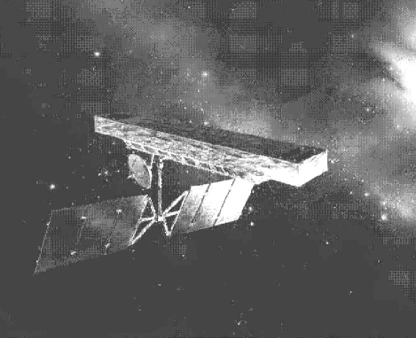
FIG. 14.: Schematic design of the SIM (Courtesy: NASA/JPL/Caltech).

VI IMAGE RECONSTRUCTION TECHNIQUES

The diffraction-limited phase retrieval of a degraded image is indeed an art. In other branches of physics too, e.g., electron microscopy, wavefront sensing, and crystallography, one often wishes to recover phase. AO systems may also require image-processing algorithms since the real-time corrected image is often partial. Prior to using such algorithms, the basic operations to be performed are dead pixel removal, debiasing, flat fielding, sky or background emission subtraction, and suppression of correlated noise. In what follows, the sub-sections VI-A to C describe methods to obtain components of the object FT and sub-section VI-D describes methods to reconstruct an image from these components, which can usually be described as a ‘deconvolution’.

A Shift-and-add algorithm

The Shift-and-add (SAA) technique (Lynds et al. 1976, Worden et al. 1976) aligns and co-adds the recorded short-exposure images; the method is analogous to the tip-tilt mirror of conventional AO systems. The position of the brightest pixel, ${\bf x}_{k}$, is necessary to be located in each specklegram, ${\cal I}_{k}({\bf x})$, [${\cal I}_{k}({\bf x}_{k})>{\cal I}_{k}({\bf x})$ for all ${\bf x}\neq{\bf x}_{k}$], followed by shifting the specklegram (without any rotation) to place this pixel at the center of the image space. The SAA image, ${\cal I}_{sa}({\bf x})$, is obtained by averaging over the set of the shifted specklegrams,

$${\cal I}_{sa}(\bf x)=<{\cal I}_{k}({\bf x}+{\bf x}_{k})>.$$ (141)

The large variations in the brightness of the brightest pixels are observed in a set of speckle images; the contamination level may not be proportional to its brightest pixel (Bates and McDonnell, 1986). The adjusted SAA image, ${\cal I}_{asa}({\bf x})$, can be defined as,

$${\cal I}_{asa}({\bf x})=<{\it w}[{\cal I}_{k}({\bf x}_{k})]{\cal I}_{k}({\bf x}+{\bf x}_{k})>,$$ (142)

where ${\it w}[{\cal I}_{k}({\bf x}_{k})]$ is the weighting in relation with the brightness of the brightest pixel. The choice of the same quantity can be made as ${\it w}\{{\cal I}_{k}({\bf x}_{k})\}={\cal I}_{k}({\bf x}_{k})$. An array of impulse is constructed by putting an impulse at each of the center of gravity with a weight proportional to the speckle intensity. This impulse array is considered to be an approximation of the instantaneous PSF and is cross-correlated with the speckle frame. Disregarding the peaks lower than the pre-set threshold, the m^th speckle mask, $mask_{m}({\bf x})$, is defined by,

$$mask_{m}({\bf x})=\sum_{n=1}^{M}{\cal I}_{m}({\bf x}_{m,n})\delta({\bf x}-{\bf x}_{m,n}).$$ (143)

The $m^{th}$ masked speckled image, $m{\cal I}_{m}({\bf x})$, is expressed as,

$$m{\cal I}_{m}({\bf x})={\cal I}_{m}({\bf x})\otimes mask_{m}({\bf x}).$$ (144)

The Lynds-Worden-Harvey image is obtained by averaging equation (127). For direct speckle imaging, the SAA image, ${\cal I}_{sa}({\bf x})$, is a contaminated one containing two complications - a convolution, ${\cal S}_{k}({\bf x})$ and an additive residual, ${\cal C}({\bf x})$ - which means,

$${\cal I}_{sa}({\bf x})={\cal O}({\bf x})\star{\cal S}({\bf x})+{\cal C}({\bf x}),$$ (145)

where ${\cal S}({\bf x})=\sum_{k=1}^{k}\delta({\bf x}-{\bf x^{\prime}}_{k})d_{k},{\bf x^{\prime}}_{k}$ being the constant position vectors and $d_{k}$, the positive constant. It is essential to calibrate ${\cal I}_{sa}({\bf x})$ with an unresolved point source and reduce it in the same way to produce ${\cal S}({\bf x})$. The estimate for the object, ${\cal O}({\bf x})$, is evaluated from the inverse FT of the following equation,

$$\widehat{\cal O}({\bf u})=\frac{\widehat{\cal I}_{sa}({\bf u})}{\widehat{\cal I}_{\circ}({\bf u})+\widehat{\cal N}({\bf u})}.$$ (146)

which is the first approximation of the object irradiance. This method is found to be insensitive to the telescope aberrations but sensitive to dominating photon noise.

Another method called ‘selective image reconstruction’ selects the few sharpest images that are recorded when the atmospheric distortion is naturally at minimum, from a large dataset of short-exposures (Dantowitz et al. 2000). Baldwin et al. (2001) have demonstrated the potential of such a technique.

B Knox-Thomson method

The Knox-Thomson (KT) method (Knox and Thomson, 1974) defines the correlation of ${\cal I}({\bf x})$ and ${\cal I}({\bf x})$ multiplied by a complex exponential factor with spatial frequency vector ${\bf\Delta u}$. The approximate phase-closure is achieved by two vectors (see figure 15), ${\bf u}$ and ${\bf u}+{\bf\Delta u}$, assuming that the pupil phase is constant over ${\bf\Delta u}$. Let the general second-order moment be the cross spectrum, $<\widehat{\cal I}({\bf u}_{1})\widehat{\cal I}^{\ast}({\bf u}_{2})>$. It takes significant values only if $|{\bf u}_{1}-{\bf u}_{2}|<r_{\circ}/\lambda$; the typical value of $|{\bf\Delta u}|$ is $\sim$0.2 - 0.5 $r_{\circ}/\lambda$. Invoking equation (70), a 2-d irradiance distribution, ${\cal I}({\bf x})$ and its FT, $\widehat{\cal I}({\bf u})$, is defined by the equation,

$$\widehat{\cal I}{\bf(u)}=\int^{+\infty}_{-\infty}{\cal I}{\bf(x)}e^{-i2\pi{\bf ux}}d{\bf x}.$$ (147)

In image space, the correlations of ${\cal I}({\bf x})$, is derived as,

$${\cal I}({\bf x}_{1},{\bf\Delta u})=\int^{+\infty}_{-\infty}{\cal I}^{\ast}({\bf x}){\cal I}({\bf x}+{\bf x}_{1})e^{i2\pi{\bf\Delta ux}}d{\bf x},$$ (148)

where ${\bf x}_{1}={\bf x}_{1x}+{\bf x}_{1y}$ are 2-d spatial co-ordinate vectors. The KT correlation may be defined in Fourier space as products of, $\widehat{\cal I}({\bf u})$,

$$\widehat{\cal I}({\bf u}_{1},{\bf\Delta u}) = \widehat{\cal I}({\bf u}_{1})\widehat{\cal I}^{\ast}({\bf u}_{1}+{\bf\Delta u}),$$ (151)

$$=\widehat{\cal O}({\bf u}_{1})\widehat{\cal O}^{\ast}({\bf u}_{1}+{\bf\Delta u})$$

$$\widehat{\cal S}({\bf u}_{1})\widehat{\cal S}^{\ast}({\bf u}_{1}+{\bf\Delta u}),$$

where ${\bf u}_{1}={\bf u}_{1x}+{\bf u}_{1y}$, and ${\bf\Delta u}={\bf\Delta u}_{x}+{\bf\Delta u}_{y}$ are 2-d spatial frequency vectors. ${\bf\Delta u}$ is a small, constant offset spatial frequency. A number of sub-planes is used by taking different values of ${\bf\Delta u}$. The argument of the equation (133) provides the phase-difference between the two spatial frequencies separated by ${\bf\Delta u}$ and is expressed as,

$$arg|\widehat{\cal I}^{KT}({\bf u}_{1},{\bf\Delta u})|=\psi({\bf u}_{1})-\psi({\bf u}_{1}+{\bf\Delta u}).$$ (152)

Therefore, the equation (133) translates into,

$$\widehat{\cal I}{(\bf u}_{1},{\bf\Delta u}) = |\widehat{\cal O}{(\bf u}_{1})||\widehat{\cal O}({\bf u}_{1}+{\bf\Delta u})|$$ (155)

$$|\widehat{\cal S}{(\bf u}_{1})||\widehat{\cal S}({\bf u}_{1}+{\bf\Delta u})|$$

$$e^{i[\theta^{KT}_{\cal O}({\bf u}_{1},{\bf\Delta u})+\theta^{KT}_{\cal S}({\bf u}_{1},{\bf\Delta u})]}.$$

The object phase-spectrum of the equation (135) is encoded in the term, $e^{i\theta^{KT}_{\cal O}({\bf u}_{1},{\bf\Delta u})}=e^{i[\psi_{\cal O}({\bf u}_{1})-\psi_{\cal O}({\bf u}_{1}+{\bf\Delta u})]}$. In a single image realization, it is corrupted by the random phase-differences due to the atmosphere-telescope OTF, $e^{i\theta^{KT}_{\cal S}({\bf u}_{1},{\bf\Delta u})}=e^{i[\psi_{\cal S}({\bf u}_{1})-\psi_{\cal S}({\bf u}_{1}+{\bf\Delta u})]}$. If equation (135) is averaged over a large number of frames, the feature $({\bf\Delta\psi_{\cal S}})=0$. $|\widehat{\cal O}({\bf u}_{1}+{\bf\Delta u})|\ \approx\ |\widehat{\cal O}({\bf u}_{1})|$, when ${\bf\Delta u}$ is small, etc., and so,

$$<\widehat{\cal I}{(\bf u}_{1},{\bf\Delta u})> = |\widehat{\cal O}({\bf u}_{1})||\widehat{\cal O}({\bf u}_{1}+{\bf\Delta u})|e^{i[\theta^{KT}_{\cal O}({\bf u}_{1},{\bf\Delta u})]}$$ (157)

$$<\widehat{\cal S}({\bf u}_{1})\widehat{\cal S}^{\ast}({\bf u}_{1}+{\bf\Delta u})>,$$

from which, together with equation (73), the object phase-spectrum, $\theta^{KT}_{\cal O}({\bf u}_{1},{\bf\Delta u})$, can be determined.

FIG. 15.: Diagrammatic representation of pupil sub-aperture of diameter, $r_{\circ}$, (a) approximate phase-closure achieved in KT method, (b) complete phase-closure is achieved in TC method.

C Triple correlation technique

The triple correlation (TC) is a generalization of closure phase technique (section IV.B.2.) that is used in radio/optical interferometry where the number of closure phases is small compared to those available from bispectrum (Weigelt, 1977, Lohmann et al. 1983). It is insensitive to (i) the atmospherically induced random phase errors, (ii) the random motion of the image centroid, and (iii) the permanent phase errors introduced by telescope aberrations; any linear phase term in the object phase cancels out as well. The images are not required to be shifted to common centroid prior to computing the bispectrum. The other advantages are: (i) it provides information about the object phases with better S/N ratio from a limited number of frames, and (ii) it serves as the means of image recovery with diluted coherent arrays (Reinheimer and Weigelt, 1987). The disadvantage of this technique is that it demands severe constraints on the computing facilities with 2-d data since the calculations are four-dimensional (4-d).

A triple correlation is obtained by multiplying a shifted object, ${\cal I}({\bf x}+{\bf x}_{1})$, with the original object, ${\cal I}({\bf x})$, followed by cross-correlating the result with the original one (for example, in the case of a close binary star, the shift is equal to the angular separation between the stars, masking one of the two components of each double speckle). The calculation of the ensemble average TC is given by,

$${\cal I}{\bf(x}_{1},{\bf x}_{2})=<\int^{+\infty}_{-\infty}{\cal I}{\bf(x)}{\cal I}({\bf x}+{\bf x}_{1}){\cal I}({\bf x}+{\bf x}_{2})d{\bf x}>,$$ (158)

where ${\bf x}_{j}={\bf x}_{jx}+{\bf x}_{jy}$ are 2-d spatial co-ordinate vectors. The bispectrum is given by,

$$\widehat{\cal I}({\bf u}_{1},{\bf u}_{2}) = <\widehat{\cal I}({\bf u}_{1})\widehat{\cal I}^{\ast}({\bf u}_{1}+{\bf u}_{2})\widehat{\cal I}({\bf u}_{2})>,$$ (161)

$$=\widehat{\cal O}({\bf u}_{1})\widehat{\cal O}^{\ast}({\bf u}_{1}+{\bf u}_{2})\widehat{\cal O}({\bf u}_{2})$$

$$<\widehat{\cal S}({\bf u}_{1})\widehat{\cal S}^{\ast}({\bf u}_{1}+{\bf u}_{2})\widehat{\cal S}({\bf u}_{2})>,$$

where ${\bf u}_{j}={\bf u}_{jx}+{\bf u}_{jy}$, $\widehat{\cal I}({\bf u}_{j})=\int{\cal I}({\bf x})e^{-i2\pi{\bf u}_{j}{\bf x}}d{\bf x}$, and

$\widehat{\cal I}^{\ast}({\bf u}_{1}+{\bf u}_{2})=\int{\cal I}({\bf x})e^{i2\pi({\bf u}_{1}+{\bf u}_{2}).{\bf x}}d{\bf x}$. The object bispectrum is given by,

$$\widehat{\cal I}_{\cal O}({\bf u}_{1},{\bf u}_{2}) = \widehat{\cal O}({\bf u}_{1})\widehat{\cal O}^{\ast}({\bf u}_{1}+{\bf u}_{2})\widehat{\cal O}({\bf u}_{2})$$ (163)

$$=\frac{<\widehat{\cal I}({\bf u}_{1})\widehat{\cal I}^{\ast}({\bf u}_{1}+{\bf u}_{2})\widehat{\cal I}({\bf u}_{2})>}{<\widehat{\cal S}({\bf u}_{1})\widehat{\cal S}^{\ast}({\bf u}_{1}+{\bf u}_{2})\widehat{\cal S}({\bf u}_{2})>}.$$

The modulus $|\widehat{\cal O}({\bf u})|$ of the object FT $\widehat{\cal O}({\bf u})$ can be evaluated from the object bispectrum $\widehat{\cal I}_{\cal O}({\bf u}_{1},{\bf u}_{2})$. The argument of equation (138) gives the phase-difference and is expressed as,

$$arg|\widehat{\cal I}^{TC}({\bf u}_{1},{\bf u}_{2})|=\psi({\bf u}_{1})+\psi({\bf u}_{2})-\psi({\bf u}_{1}+{\bf u}_{2}).$$ (164)

The object phase-spectrum is encoded in the term $e^{i\theta^{TC}_{\cal O}({\bf u}_{1},{\bf u}_{2})}$. It is corrupted in a single realization by the random phase-differences due to the atmosphere-telescope OTF, $e^{i\theta^{TC}_{\cal S}({\bf u}_{1},{\bf u}_{2})}=e^{i[\psi_{\cal S}({\bf u}_{1})-\psi_{\cal S}({\bf u}_{1}+{\bf u}_{2})+\psi_{\cal S}({\bf u}_{2})]}$. If sufficient number of specklegrams are averaged, one can overcome this shortcoming. Let $\theta^{TC}_{\cal O}({\bf u}_{1},{\bf u}_{2})$ be the phase of the object bispectrum; then,

$$\widehat{\cal O}({\bf u}) = |\widehat{\cal O}({\bf u})|e^{i\psi({\bf u})},$$ (165)

$$\widehat{\cal I}_{\cal O}({\bf u}_{1},{\bf u}_{2}) = |\widehat{\cal I}_{\cal O}({\bf u}_{1},{\bf u}_{2})|e^{i\theta^{TC}_{\cal O}({\bf u}_{1},{\bf u}_{2})}.$$ (166)

Equations (142) and (143) may be inserted into equation (140), yielding the relations,

$$\widehat{\cal I}_{\cal O}({\bf u}_{1},{\bf u}_{2}) = |\widehat{\cal O}({\bf u}_{1})||\widehat{\cal O}({\bf u}_{2})||\widehat{\cal O}({\bf u}_{1}+{\bf u}_{2})|$$ (168)

$$e^{i[\psi_{\cal O}({\bf u}_{1})-\psi_{\cal O}({\bf u}_{1}+{\bf u}_{2})+\psi_{\cal O}({\bf u}_{2})]}\rightarrow,$$

$$\theta^{TC}_{\cal O}({\bf u}_{1},{\bf u}_{2}) = \psi_{\cal O}({\bf u}_{1})-\psi_{\cal O}({\bf u}_{1}+{\bf u}_{2})+\psi_{\cal O}({\bf u}_{2}).$$ (169)

Equation (145) is a recursive one for evaluating the phase of the object FT at coordinate ${\bf u}={\bf u}_{1}+{\bf u}_{2}$. The reconstruction of the object phase-spectrum from the phase of the bispectrum is recursive in nature. The object phase-spectrum at $({\bf u}_{1}+{\bf u}_{2})$ can be written as,

$$\psi_{\cal O}({\bf u}_{1}+{\bf u}_{2})=\psi_{\cal O}({\bf u}_{1})+\psi_{\cal O}({\bf u}_{2})-\theta^{TC}_{\cal O}({\bf u}_{1},{\bf u}_{2}).$$ (170)

If the object spectrum at ${\bf u}_{1}$ and ${\bf u}_{2}$ is known, the object phase-spectrum at $({\bf u}_{1}+{\bf u}_{2})$ can be computed. The bispectrum phases are mod $2\pi$, therefore, the recursive reconstruction in equation (139) may lead to $\pi$ phase mismatches between the computed phase-spectrum values along different paths to the same point in frequency space. However, according to Northcott et al. (1988), phases from different paths to the same point cannot be averaged to reduce noise under this condition. A variation of the nature of computing argument of the term, $e^{i\psi_{\cal O}({\bf u}_{1}+{\bf u}_{2})}$, is needed to obtain the object phase-spectrum and the equation (146) translates into,

$$e^{i\psi_{\cal O}({\bf u}_{1}+{\bf u}_{2})}=e^{i[\psi_{\cal O}({\bf u}_{1})+\psi_{\cal O}({\bf u}_{2})-\theta^{TC}_{\cal O}({\bf u}_{1},{\bf u}_{2})]}.$$ (171)

The values obtained using the unit amplitude phasor recursive re-constructor are insensitive to the $\pi$ phase ambiguities. Saha et al. (1999) have developed a code based on this re-constructor. The least-square formulation of the phase reconstruction (Glindemann et al. 1991) and the projection-slice theorem of tomography and the Radon transform (Northcott et al. 1988) have been successfully applied in the development of phase reconstruction from the bispectrum.

D Deconvolution algorithms

Most deconvolution techniques, in which ‘a priori information’ plays an essential role, can be simplified to the minimization /maximization of a criterion by using an iterative numerical method (Gerchberg and Saxton, 1972) that bounces back and forth between the image-domain and Fourier-domain constraints until two images are found that produce the input image when convolved together (Ayers and Dainty, 1988).

1 Blind iterative deconvolution (BID) technique

Let the degraded image, ${\cal I}({\bf x})$, be used as the operand. An initial estimate of the PSF, ${\cal S}({\bf x})$, has to be provided. The image is deconvolved from the guess PSF by Wiener filtering (see section IV.A.1), which is an operation of multiplying a suitable Wiener filter (constructed from $\widehat{\cal S}({\bf u})$, of the PSF) with $\widehat{\cal I}({\bf u})$. The technique of Wiener filtering damps the high frequencies and minimizes the mean square error between each estimate and the true spectrum. This filtered deconvolution takes the form,

$$\widehat{\cal O}({\bf u})=\widehat{\cal I}({\bf u)}{\frac{\widehat{\cal O}_{f}({\bf u})}{\widehat{\cal S}({\bf u})}}.$$ (172)

The Wiener filter, $\widehat{\cal O}_{f}({\bf u})$, is derived as,

$${\widehat{\cal O}_{f}({\bf u})={\frac{\widehat{\cal S}({\bf u})\widehat{\cal S}^{\ast}({\bf u})}{|\widehat{\cal S}({\bf u})|^{2}+|\widehat{\cal N}({\bf u})|^{2}}}}.$$ (173)

The term, $\widehat{\cal N}({\bf u})$ can be replaced with a constant estimated as the rms fluctuation of the high frequency region in the spectrum where the object power is negligible. The Wiener filtering spectrum, $\widehat{\cal O}(\bf u)$, takes the form:

$$\widehat{\cal O}({\bf u})=\widehat{\cal I}({\bf u}){\frac{\widehat{\cal S}^{\ast}({\bf u})}{\widehat{\cal S}({\bf u})\widehat{\cal S}^{\ast}({\bf u})+\widehat{\cal N}({\bf u})\widehat{\cal N}^{\ast}({\bf u})}}.$$ (174)

The result, $\widehat{\cal O}({\bf u})$, is transformed back to image space, the negatives in the image and the positives outside a prescribed domain (called object support) are set to zero. The average of negative intensities within the support are subtracted from all pixels. The process is repeated until the negative intensities decrease below the noise. A new estimate of the PSF is next obtained by Wiener filtering ${\cal I}({\bf x})$, with a filter constructed from the constrained object, ${\cal O}({\bf x})$; this completes one iteration. This entire process is repeated until the derived values of ${\cal O}({\bf x})$ and ${\cal S}({\bf x})$ converge to sensible solutions.

BID has the ability to retrieve the diffraction-limited image of an object from a single specklegram without the reference star data (Saha and Venkatakrishnan, 1997). Jefferies and Christou, (1993), have developed an algorithm which requires more than a single speckle frame for improving the convergence. Barnaby et al. (2000) used this algorithm, and parametric blind deconvolution (PBD) to post-process the data obtained with the AO system, and found that the secondary of 81 Cnc was 0.12 $m_{v}$ brighter than the primary at 0.85 $\mu$m.

2 Fienup algorithm

Fienup (1978) algorithm reconstructs an object using only the modulus of its FT. At the $kth$ iteration, ${\cal G}_{k}{(\bf x)}$, an estimate of the object FT, is compared with the measured one and made to conform with the modulus at all Fourier frequencies. The inverse transform of the result yields an image ${\cal G}_{k}^{\prime}{(\bf x)}$. This iteration is completed by forming a new estimate of the object that conforms to certain object-domain constraints, e.g., positivity and finite extent, such that,

$$\widehat{\cal G}_{k}{(\bf u)} = |\widehat{\cal G}_{k}{(\bf u)}|e^{i\phi_{k}{(\bf u)}}={\cal F}[{\cal G}_{k}{(\bf x)}],$$ (175)

$$\widehat{\cal G}_{k}^{\prime}{(\bf u)} = |\widehat{\cal I}{(\bf u)}|e^{i\phi_{k}{(\bf u)}},$$ (176)

$${\cal G}_{k}^{\prime}{(\bf x)} = {\cal F}^{-1}[\widehat{\cal G}_{k}^{\prime}{(\bf u)}],$$ (177)

$${\cal G}_{k+1}({\bf x}) = {\cal G}_{k}^{\prime}({\bf x}),\,\,\,{\bf x}\notin\gamma,$$ (179)

$$=0,\,\,\,\,\,\,\,\,\,\,{\bf x}\in\gamma,$$

where the region $\gamma$ is the set of all points at which ${\cal G}_{k}^{\prime}{(\bf x)}$ violates the object-domain constraints, and ${\cal G}_{k}{(\bf x)},\widehat{\cal G}_{k}^{\prime}{(\bf u)}$, and $\phi_{k}$ are estimates of ${\cal I}{(\bf x)},\widehat{\cal I}{(\bf u)}$, and the phase $\psi$ of $\widehat{\cal I}{(\bf u)}$, respectively.

The above procedure may be accelerated if an estimate, ${\cal G}_{k+1}{(\bf x)}$ is formed as,

$${\cal G}_{k+1}({\bf x}) = {\cal G}_{k}{(\bf x)},\,\,\,\,\,\,\,\,\,\,\,\,\,\,\,\,\,\,\,\,\,\,\,\,\,\,\,\,\,{\bf x}\notin\gamma,$$ (181)

$$={\cal G}_{k}{(\bf x)}-\beta{\cal G}_{k}^{\prime}{(\bf x)},\,\,\,{\bf x}\in\gamma,$$

where $\beta$ is a constant feedback parameter.

3 Other iterative algorithms

I. The Richardson-Lucy (Richardson, 1972, Lucy, 1974) algorithm converges to the maximum likelihood solution for Poisson statistics in the data which is appropriate for optical data with noise from counting statistics. It forces the restored image to be non-negative and conserves flux both globally and locally at each iteration.

II. The Magain, Courbin, Sohy, (MCS; Magain et al. 1998) algorithm is based on the principle that sampled data cannot be fully deconvolved without violating the sampling theorem (Shannon, 1949) that determines the maximal sampling interval allowed so that an entire function can be reconstructed from sampled data. The sampled image should be deconvolved by a narrower function instead of the total PSF so that the resolution of the deconvolved image is compatible with the adopted sampling. The positivity constraint unlike the traditional deconvolution methods, is not mandatory; accurate astrometric and photometric informations of the astronomical objects can be obtained.

III. The myopic iterative step preserving algorithm, (MISTRAL; Conan et al. 1998), is based on the Bayesian theorem that uses the probabilistic approach. It incorporates a positivity constraint and some a priori knowledge of the object (an estimate of its local mean and a model for the power spectral density etc.). It also allows one to account for the noise in the image, the imprecise knowledge of the PSF. MISTRAL has produced a few spectacular images after processing AO images.

IV. A non-linear iterative image reconstruction algorithm, called Pixon method has been developed by Puetter and Yahil (1999) that provides statistically unbiased photometry and robust rejection of spurious sources. Unlike other Bayesian methods, this technique does not assign explicit prior probabilities to image models. It minimizes complexity by smoothing the image model locally. The model is then described using a few irregular-sized pixons containing similar amounts of information, rather than many regular pixels containing variable signal-to-noise data. Eke (2001) opines that it has the ability to detect sources in low SNR data and to deconvolve a telescope beam in order to recover the internal structure of a source.

4 Aperture-synthesis mapping

Reconstruction of complex images involves the knowledge of complex visibilities. Interferometers with two apertures have limited possibilities for image reconstructions due to absence of phase visibility recovering. The phase of a visibility may be deduced from closure-phase that has been applied in optical interferometry (Baldwin et al. 1998). Process after data acquisition consists of phase calibration and visibility phase reconstruction from closure-phase terms by technique similar to bispectrum processing. From complex visibilities acquired from a phased interferometric array , it is possible to reconstruct the image by actually interpolating the function in the $(u,v)$ plane. Let the output of a synthesis array be a set of visibility functions ${\cal V}(u_{j},v_{j})$ that are obtained by averaging the quasi-sinusoidal response of each interferometer pair and hence, the resultant brightness distribution be given by the equation:

$${\cal I}^{\prime\prime}(x,y)=\sum_{j=1}^{N}{\cal V}(u_{j},v_{j}){\it w}_{j}e^{[-2\pi i(u_{j}x+v_{j}y)]},$$ (182)

where ${\cal I}^{\prime\prime}(x,y)$ is usually called the dirty image which is the convolution of the true brightness distribution ${\cal I}^{\prime}(x,y)$ with the synthesized beam ${\cal S}^{\prime}(x,y)$, ${\it w}_{j}$ is a weight associated with $j^{th}N$. The map will show sufficient details when the $(u,v)$ coverage is good, but it is not the best representation of the sky and contains many artifacts notably the positive and negative side lobes around bright peaks. If the sampling of the $(u,v)$ plane is irregular and uneven, the dirty beam will have large sidelobes and confuse and obscure the structure of interest in the image.

Several non-linear methods have been introduced to restore the unmeasured Fourier components in order to produce a more physical map. These methods work on the constraint that the image must be everywhere positive or zero and they make use of a priori knowledge about the extent of the source and statistics of the measurement processes. Since the restoration is not unique, the image restoration must select the best solution.

a CLEAN

The most commonly used approaches to deconvolve dirty image fall into two groups: CLEAN algorithms (Högbom, 1974) and maximum-entropy methods (MEM, Ables, 1974). To some extent, CLEAN and MEM are complimentary in their application. Between them, CLEAN is the most routinely used algorithm, particularly in radio astronomy, because it is both computationally efficient and intuitively easy to understand. This procedure is a non-linear technique that applies iterative beam removing method. It starts with a dirty image ${\cal I}^{\prime}(x,y)$ made by the linear Fourier inversion procedure and attempts to decompose this image into a number of components, each of which contains part of the dirty beam ${\cal S}^{\prime}(x,y)$. One wishes to determine the set of numbers ${\cal A}_{i}(x_{i},y_{i})$ such that

$${\cal I}^{\prime}(x,y)=\sum_{i}{\cal A}_{i}{\cal S}^{\prime}(x-x_{i},y-y_{i})+{\cal I}_{R}(x,y),$$ (183)

where ${\cal I}_{R}(x,y)$ is the residual brightness distribution after the decomposition. The solution is considered satisfactory if ${\cal I}_{R}(x,y)$ is of the order of the expected noise.

The algorithm searches the dirty image for the pixel with largest absolute value ${\cal I}_{max}$ and subtracts a dirty beam pattern centered on this point with amplitude $G_{l}{\cal I}_{max}$, where $G_{l}$ is called the loop gain. The residual map is searched for the next largest value and the second beam stage is subtracted and so on. The iteration is stopped when the maximum residual is consistent with the noise level. The iteration consists of a residual image that contains noise and low level source calculations plus a set of amplitudes and positions of the components removed. These components can be considered as an array of delta function and convolved with a clean beams and added to produce a CLEANed image. The clean beam is usually chosen as a truncated elliptical Gaussian about the same size of the main lobe of the dirty beam. CLEAN results in a map with the same resolution as the original dirty map without sidelobes.

b Maximum entropy method (MEM)

It is found that CLEAN generally performs well on small compact sources, while MEM does better on extended sources. MEM is employed in a variety of fields like medical imaging, crystallography, radio and X-ray astronomy as well. This procedure governs the estimation of probability distributions when limited information is available. In addition, it treats all the polarization component images simultaneously (unlike CLEAN which deconvolves different polarization component images independently) and guarantees essential conditions on the image. It makes use of the highest spatial frequency information by finding the smoothest image consistent with the interferometric data. While enforcing positivity and conserving the total flux in the frame, smoothness is estimated by the ‘entropy’ $S$ that is of the form,

$$S=-\sum_{i}{\it h}_{j}\ln\frac{{\it h}_{j}}{{\it m}_{j}},$$ (184)

where ${\bf h}=[{\it h}_{j}]$ represents the image to be restored, and ${\bf m}=[{\it m}_{j}]$ is known as prior image.

It can be shown that $S\leq 0$; the equality holds if ${\bf h}={\bf m}$. The value of $S$ is a measure of the similarity between ${\bf h}$ and ${\bf m}$ if the entropy $S$ is maximized without any data constraints. With data constraints, the maximum of $S$ will be less than its absolute maximum value zero, meaning that ${\bf h}$ has been modified and deviated from its prior model ${\bf m}$.

MEM solves the multi-dimensional constraints minimization problem. It uses only those measured data and derives a brightness distribution which is the most random, i.e., has the maximum entropy $S$ of any brightness distribution consistent with the measured data. Maintaining an adequate fit to the data, it reconstructs the final image that fits the data within the noise level.

Monnier et al. (2001) have reconstructed the dust shells around two evolved stars, IK Tau and VY CMa using $(u,v)$ coverage from the contemporaneous observations at Keck-I and IOTA. Figure 16 depicts the MEM reconstructions of the dust shells around these stars. Their results clearly indicate that without adequate spatial resolution, it is improbable to cleanly separate out the contributions of the star from the hot inner radius of the shell (left panel in figure 16). They opined that image reconstructions from the interferometer data are not unique and yield results which depend heavily on the biases of a given reconstruction algorithm. By including the long baselines ($>$ 20 m) data from the IOTA interferometer (right panel), the fraction of the flux arising from the central star can be included in the image reconstruction process by using the MEM prior. One can see for a dust shell such as IK Tau, that additional IOTA data are critical in accurately interpreting the physical meaning of interferometer data. The thick dashed lines show the expected dust shell inner radius from the data obtained at the ISI.

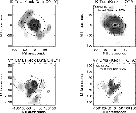
FIG. 16.: MEM image reconstructions of the dust shell around IK Tau and VY CMa (Courtesy: J. D. Monnier); the left panels show the reconstructions of them from data obtained with a single Keck telescopes using aperture masking (baselines up to 9 m at 2.2 $\mu$m, and the right panels show the dust shell reconstructions when the fractional amounts of star and dust shell emission is constrained to be consistent with both the Keck and IOTA data (Monnier et al. 2001).

c Self calibration

In case of producing images with accurate visibility amplitude and poor or absence of phases, self calibration can be used (Baldwin and Warner, 1976). Cornwell and Wilkinson, 1981) introduced a modification by explicitly solving for the telescope-specific error as part of the reconstructing step. The measured Fourier phases are fit using a combination of intrinsic phases plus telescope phase errors.

If the field of observation contains one dominating internal point source which can be used as an internal phase reference, the visibility phase at other spatial frequencies is derived. A hybrid map can be made with the measured amplitudes together with model phase distributions. Since the measured amplitudes differ from the single point source model, the hybrid map diffuses from the model map. Adding some new feature to the original model map, an improved model map is obtained in the next iteration. With clever selection of features to be added to the model in each iteration, the procedure converges.

d Linear approach

Another approach to the deconvolution problem is to formulate it as a linear system of the form:

$${\bf Ax}={\bf b},$$ (185)

and then use algebraic techniques to solve this system. The elements of A contain samples of the dirty beam, the elements of b are samples of the dirty image, while x contains components of the reconstructed image. Without any additional constraints matrix A is singular: additional information has to be added to find a solution. Assumptions that regularize the system include positivity and compact structure of the source. An algebraic approach is not new in itself, but practical applications of such techniques in astronomy have become feasible only recently, e.g., for the non-negative least squares (NNLS, Briggs, 1995).

e WIPE

Lannes et al. (1994) present another technique, WIPE, based on a least squares approach, where support information is used to regularize the algorithm. Again, a linear system similar to that mentioned in the previous paragraph is solved, but using a technique which iterates between ($u,v$) and image-planes. Unlike CLEAN and MEM, WIPE suppresses excessive extrapolation of higher spatial frequencies during the deconvolution.

VII ASTRONOMICAL APPLICATIONS

Optical interferometry in astronomy is a boon for astrophysical studies. The following sub-sections dwell on the astrophysical importance and the perspectives of interferometry.

A Results from single aperture interferometry

Single aperture interferometry has been contributing to study of the Sun and solar system, and of a variety of stellar astrophysical problems.

1 Sun and solar system

The existence of solar features with sizes of the order of 100 km or smaller was found by means of speckle imaging (Harvey, 1972, Harvey and Breckinridge, 1973). From observations of photospheric granulation from disk center to limb at $\lambda=550\pm 5~{}nm$, Wilken et al. (1997) found a decrease of the relative rms-contrast of the center-to-limb of the granular intensity. A time series of high spatial resolution images reveal the highly dynamical evolution of sunspot fine structure, namely, umbral dots, penumbral filaments, facular points (Denker, 1998). Small-scale brightening in the vicinity of sunspots, were also observed in the wings of strong chromospheric absorption lines. These structures which are concomitant with strong magnetic fields show brightness variations close to the diffraction-limit of the Vacuum Tower Telescope ($\sim$0.16^′′ at 550 nm), Observatorio del Teide (Tenerife). With the phase-diverse speckle method, Seldin et al. (1996) found that the photosphere at scales below 0.3^′′ is highly dynamic.

Speckle imaging has been successful in resolving the heavenly dance of Pluto-Charon system (Bonneau and Foy, 1980), as well as in determining shapes of asteroids (Drummond et al. 1988). Reconstructions of Jupiter with sub-arcsecond resolution have also been carried out by Saha et al. (1997).

2 Stellar objects

Studies of close binary stars play a fundamental role in measuring stellar masses, providing a benchmark for stellar evolution calculations; a long term benefit of interferometric imaging is a better calibration of the main-sequence mass-luminosity relationship. The parameter in obtaining masses involves combining the spectroscopic orbit with the astrometric orbit from the interferometric data. Continuous observations are necessary to be carried out in order to derive accurate orbital elements and masses, luminosities and distances. The radiative transfer concerning the effects of irradiation on the line formation in the expanding atmospheres of the component that is distorted mainly by physical effects, viz.,(i) rotation of the component, and (ii) the tidal effect can be modeled as well. More than 8000 interferometric observations of stellar objects have been reported so far, out of which 75% are of binary stars (Hartkopf et al. 1997). The separation of most of the new components discovered are found to be less than 0.25^′′. From an inspection of the interferometric data, Mason et al. (1999) have confirmed the binary nature of 848 objects, discovered by the Hipparcos satellites; Prieur et al. (2001) reported high angular resolution astrometric data of 43 binary stars that were also observed with same satellite. Torres et al. (1997) derived individual masses for $\theta^{1}$ Tau using the distance information from $\theta^{2}$ Tau; they found that the empirical mass-luminosity relation in good agreement with theoretical models. Gies et al. (1997) measured the radial velocity for the massive binary 15 Mon. With the speckle spectrograph, Baba, Kuwamura, Miura et al. (1994) have observed a binary star, $\phi$ And ($\rho$ = 0.53^′′) and found that the primary (a Be star) has H$\alpha$ in emission while the companion has H$\alpha$ in absorption. The high angular polarization measurements of the pre-main sequence binary system Z CMa at 2.2 $\mu$m by Fischer et al. (1998) reveal that both the components are polarized; the secondary showed an unexpected by large degree of polarization.

Studies of multiple stars are also an important aspect that can reveal mysteries. For instance, the R136a was thought to be a very massive star with a mass of $\sim$2500M_⊙ (Cassinelli et al. 1981). Speckle imagery revealed that R136a was a dense cluster of stars (Weigelt and Baier, 1985, Pehlemann et al. 1992). R64 (Schertl et al. 1996), HD97950, and the central object of giant HII region starburst cluster NGC3603 (Hofmann et al. 1995) have been observed as well. The star-like luminous blue variable (LBV), $\eta$ Carinae, an intriguing massive southern object, was found to be a multiple object (Weigelt and Ebersberger, 1986). The polarimetric reconstructed images with a 0.11^′′ resolution in the H$\alpha$ line of $\eta$ Carina exhibit a compact structure elongated in consistence with the presence of a circumstellar equatorial disk (Falcke et al. 1996).

Many supergiants have extended gaseous envelope which can be imaged in their chromospheric lines. The diameter of a few such objects, $\alpha$ Ori and Mira, are found to be wavelength dependent (Bonneau and Labeyrie, 1973, Labeyrie et al. 1977, Weigelt et al. 1996). Recent studies have also confirmed the asymmetries on their surfaces; the presence of hotspots are reported as well (Wilson et al. 1992, Haniff et al. 1995, Bedding, Zijlstra et al. 1997, Tuthill et al. 1997, Monnier et al. 1999, Tuthill, Monnier et al. 1999). The surface imaging of long period variable stars (Tuthill, Haniff et al. 1999), VY CMA reveals non-spherical circumstellar envelope (Wittkowski, Langer et al. 1998). Monnier et al. (1999) have found emission to be one-sided, inhomogeneous and asymmetric in IR and derived the line-of-sight optical depths of its circumstellar dust shell. The radiative transfer modeling of the supergiant NML Cyg reveals the multiple dust shell structures (Blöcker et al. 2001).

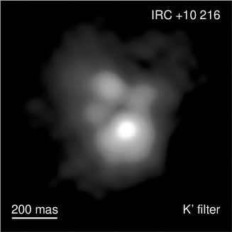
FIG. 17.: Speckle masking reconstruction of IRC+10216 (Courtesy: R. Osterbart); the resolution of the object is found to be 76 mas for the K^′ band (Osterbart et al. 1996).

High resolution imagery may depict the spatial distribution of circumstellar matter surrounding objects which eject mass, particularly in young compact planetary nebula (YPN) or newly formed stars in addition to T Tauri stars, late-type giants or supergiants. The large, older and evolved planetary nebula (PN) show a great variety of structure (Balick, 1987) that are (a) spherically symmetric (A39), (b) filamentary (NGC6543), (c) bipolar (NGC6302), and (d) peculiar (A35). The structure may form in the very early phases of the formation of the nebula itself which is very compact and unresolved. By making maps at many epochs, as well as by following the motion of specific structural features, one would be able to understand the dynamical processes at work. The structures could be different in different spectral lines e.g., ionization stratification in NGC6720 (Hawley and Miller, 1977), and hence maps can be made in various atomic and ionic emission lines too. Major results, such as, (i) measuring angular diameters of several YPNs (Barlow et al. 1986, Wood et al. 1986). (ii) resolving five individual clouds around carbon star IRC+10216 (see figure 17) with a central peak surrounded by patchy circumstellar matter (Osterbart et al. 1996, Weigelt et al. 1998), (iii) exhibiting two lobes of the evolved object, the Red Rectangle (see figure 18) (Osterbart et al. 1996), (iv) revealing a spiral pinwheel in the dust around WR104 (Tuthill, Monnier et al. 1999), and (v) depicting spherical dust shell around oxygen-rich AGB star AFGL 2290 (Gauger et al. 1999) are to be noted; images of the young star, LkH$\alpha$ 101 in which the structure of the inner accretion disk is resolved have been reported as well (Tuthill et al. 2001). Detailed information that is needed for the modeling of the 2-d radiative transfer concerning the symmetry $-$ spherical, axial or lack of clouds, plumes etc. of the objects $-$ can also be determined (Men’shchikov and Henning, 1997, Gauger et al. 1999).

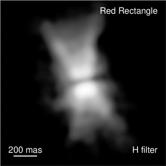
FIG. 18.: Speckle masking reconstruction of reflection nebula around the star HD44179, of Red Rectangle Red Rectangle (AFGL 915) exhibiting two lobes with $\rho$ = $\sim$0.15^′′ (Courtesy: R. Osterbart); the dark lane between the lobes might be due to an obscuring dust disk and the central star is a close binary system (Osterbart et al. 1996).

Both novae and supernovae (SN) have a complex nature of shells viz., multiple, secondary and asymmetric. High resolution mapping may depict the events near the star and the interaction zones between gas clouds with different velocities. Soon after the explosion of the supernova SN1987A, various observers monitored routinely the expansion of the shell in different wavelengths (Nisenson et al. 1987, Papaliolios et al. 1989, Wood et al. 1989). The increasing diameter of the same in several spectral lines and the continuum was measured (Karovska et al. 1989). Nulsen et al. (1990) have derived the velocity of the expansion as well and found that the size of this object was strongly wavelength dependent at the early epoch $-$ pre-nebular phase indicating stratification in its envelope. A bright source at 0.06^′′ away from the SN1987A with $\Delta m$ 2.7 mag at H$\alpha$ had also been detected. Recently, Nisenson and Papaliolios (1999) have detected a faint second spot, $\Delta m_{v}$ 4.2 mag, on the opposite side of SN1987A with $\rho$ = 160 mas.

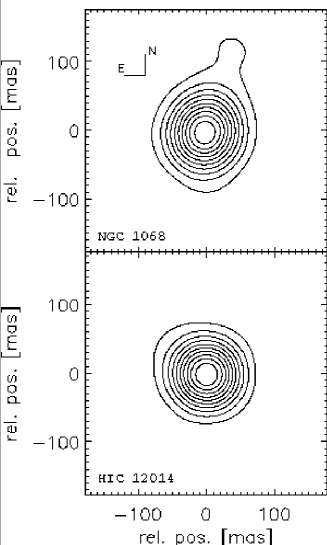
FIG. 19.: Speckle masking reconstruction of NGC1068 (top) and the unresolved star HIC12014 (bottom). The contours are from 6% to 100% of peak intensity (Wittkowski, Balega et al. 1998; Courtesy: M. Wittkowski).

Another important field of observational astronomy is the study of the physical processes, viz., temperature, density and velocity of gas in the active regions of active galactic nuclei (AGN); optical imaging by emission lines on sub-arcsecond scales can reveal the structure of the narrow-line region. The scale of narrow-line regions is well resolved by the diffraction-limit of a moderate-sized telescope. The time variability of AGNs ranging from minutes to decades can also be studied. The NGC 1068 is an archetype type 2 Seyfert galaxy. Observations of this object corroborated with theoretical modeling like radiative transfer calculations have made significant contributions on its structure. Ebstein et al. (1989) found a bipolar structure of this object in the [OIII] emission line. Near-IR observations at the Keck I telescope trace a very compact central core and extended emission with a size of the order of 10 pc on either side of an unresolved nucleus (Weinberger et al. 1999). Wittkowski, Balega et al. (1998) have resolved central 2.2 $\mu$m core by bispectrum speckle interferometry at the diffraction-limit of the Special Astrophysical Observatory (SAO) 6 m telescope, with a FWHM size of $\sim$2 pc for an assumed Gaussian intensity distribution. Figure 19 depicts the reconstructed image of the AGN, NGC1068. Subsequent observations by Wittkowski et al. (1999) indicate that this compact core is asymmetric with a position angle of $\sim$20^∘ and an additional more extended structure in N-S direction out to $\sim$25 pc.

Quasars (QSO) may be gravitationally lensed by stellar objects such as, stars, galaxies, clusters of galaxies etc., located along the line of sight. The aim of the high angular imagery of these QSOs is to find their structure and components; their number and structure as a probe of the distribution of the mass in the Universe. The capability of resolving these objects in the range of 0.2^′′ to 0.6^′′ would allow the discovery of more lensing events. The gravitational image of the multiple QSO PG1115+08 was resolved by Foy et al. (1985); one of the bright components, discovered to be double (Hege et al. 1981), was found to be elongated that might be, according to them, due to a fifth component of the QSO.

3 Glimpses of AO observations

Most of the results that obtained from the ground-based telescopes equipped with AO systems are in the near-IR band; while results at visible wave lengths continue to be sparse. The contributions are in the form of studying (i) planetary meteorology (Poulet and Sicardy, 1996, Marco et al. 1997, Roddier et al. 1997); images of Neptune’s ring arcs are obtained (Sicardy et al. 1999) that are interpreted as gravitational effects by one or more moons, (ii) nucleus of M31 (Davidge, Rigaut et al. 1997), (iii) young stars and multiple star systems (Bouvier et al. 1997), (iv) galactic center (Davidge, Simons et al. 1997), (v) Seyfert galaxies, QSO host galaxies (Hutchings et al. 1998, 1999), and (vi) circumstellar environment (Roddier et al. 1996). The images of the objects such as, (a) the nuclear region of NGC3690 in the interacting galaxy Arp 299 (Lai et al. 1999), (b) the starburst/AGNs, NGC863, NGC7469, NGC1365, NGC1068, (c) the core of the globular cluster M13 (Lloyd-Hart et al. 1998). and (d) R136 (Brandl et al. (1996) etc. are obtained from the moderate-sized telescopes. The highest ever angular resolution AO images of the radio galaxy 3C294 in the near-IR bands have been obtained at Keck Observatory (Quirrenbach et al. 2001).

AO systems can also employed for studying young stars, multiple stars, natal disks, and related inward flows, jets and related outward flows, proto-planetary disks, brown dwarfs and planets. Roddier et al. (1996) have detected a binary system consisting of a K7-MO star with an M4 companion that rotates clockwise; they suggest that the system might be surrounded by a warm unresolved disk. The massive star Sanduleak-66^∘41 in the LMC was resolved into 12 components by Heydari and Beuzit (1994). Success in resolving companions to nearby dwarfs has been reported (Beuzit et al. 2001, Kenworthy et al. 2001). Macintosh et al. (2001) measured the position of the brown dwarf companion to TWA5 and resolved the primary into an 0.055^′′ double.

The improved resolution of crowded fields like globular clusters would allow derivation of luminosity functions and spectral type, to analyze proper motions in their central area. Simon et al. (1999) have detected 292 stars in the dense Trapezium star cluster of the Orion nebula and resolved pairs to the diffraction-limit of a 2.2 m telescope. Optical and near-IR observations of the close Herbig Ae/Be binary star NX Pup (Brandner et al. 1995), associated with the cometary globular cluster I, Schöller et al. (1996) estimated the mass and age of both the components and suggest that circumstellar matter around the former could be described by a viscous accretion disk. Line and continuum fluxes, and equivalent widths are also derived for the massive stars in the Arches cluster (Blum et al. 2001).

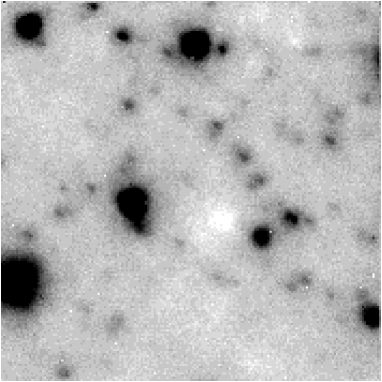
FIG. 20.: The ADONIS K^′ image of the Sgr window in the bulge of the Milky Way (Bedding, Minniti et al. 1997). The image is 8^′′$\times$8^′′ (Courtesy: T. Bedding).

Stellar populations in galaxies in near-IR region provides the peak of the spectral energy distribution for old populations. Bedding, Minniti et al. (1997) have observed the Sgr A window at the Galactic center of the Milky Way. They have produced an IR luminosity function and color-magnitude diagram for 70 stars down to $m_{v}\simeq$19.5 mag. Figure 20 depicts the ADONIS K^′ image of the Sgr A window.

Images have been obtained of the star forming region Messier 16 (Currie et al. 1996), the reflection nebula NGC2023 revealing small-scale structure in the associated molecular cloud, close to the exciting star, in Orion (Rouan et al. 1997). Close et al. (1997) mapped near-IR polarimetric observations of the reflection nebula R Mon resolving a faint source, 0.69^′′ away from R Mon and identified it as a T Tauri star. Monnier et al. (1999) found a variety of dust condensations that include a large scattering plume, a bow shaped dust feature around the red supergiant VY CMa; a bright knot of emission 1^′′ away from the star is also reported. They argued in favor of the presence of chaotic and violent dust formation processes around the star. Imaging of proto-planetary nebula (PPN), Frosty Leo and the Red Rectangle by Roddier et al. (1995) revealed a binary star at the origin of these PPNs.

Imaging of the extragalactic objects particularly the central area of active galaxies where cold molecular gas and star formation occur is an important program. From the images of nucleus of NGC1068, Rouan et al. (1998), found several components that include: (i) an unresolved conspicuous core, (ii) an elongated structure, and (iii) large and small-scale spiral structures. Lai et al. (1998) have recorded images of Markarian 231, a galaxy 160 Mpc away demonstrating the limits of achievements in terms of morphological structures of distant objects.

Aretxaga et al. (1998) reported the unambiguous detection of the host galaxy of a normal radio-quiet QSO at high-redshift in K-band; detection of emission line gas within the host galaxies of high redshift QSOs has been reported as well (Hutchings et al. 2001). Observations by Ledoux et al. (1998) of broad absorption line quasar APM 08279+5255 at z=3.87 show the object consists of a double source ($\rho$ = 0.35^′′ $\pm$ 0.02^′′; intensity ratio = 1.21 $\pm$ 0.25 in H band). They proposed for a gravitational lensing hypothesis which came from the uniformity of the quasar spectrum as a function of the spatial position. Search for molecular gas in high redshift normal galaxies in the foreground of the gravitationally lensed quasar Q1208+1011 has also been made (Sams et al. 1996). AO imaging of a few low and intermediate redshift quasars has been reported recently (Márquez et al. 2001).

High resolution stellar coronagraphy is of paramount importance in (i) detecting low mass companions, e.g., both white and brown dwarfs, dust shells around asymptotic giant branch (AGB) and post-AGB stars, (ii) observing nebulosities leading to the formation of a planetary system, ejected envelops, accretion disk, and (iii) understanding of structure (torus, disk, jets, star forming regions), and dynamical process in the environment of AGNs and QSOs. By means of coronagraphic techniques the environs of a few interesting objects have been explored. They include: (i) a very low mass companion to the astrometric binary Gliese 105 A (Golimowski et al. 1995), (ii) a warp of the circumstellar disk around the star $\beta$ Pic (Mouillet et al. 1997), (iii) highly asymmetric features in AG Carina’s circumstellar environment (Nota et al. 1992), (iv) bipolar nebula around the LBV R127 (Clampin et al. 1993), and (v) the remnant envelope of star formation around pre-main sequence stars (Nakajima and Golimowski, 1995).

B Impact of LBOIs in astrophysics

The main objective of LBOIs is to measure the diameters, distances, masses and luminosities of stars, to detect the morphological details, such as granulations, oblateness of giant stars, and the image features, i.e., spots and flares on their surfaces. Eclipsing binaries are also good candidates; for they provide information on circumstellar envelopes such as, the diameter of inner envelope, color, symmetry, radial profile etc. As stated earlier (in section VII.A.2), good spectroscopic and interferometric measurements are required to derive precise stellar masses since they depend on $sin^{3}i$. A small variation on the inclination $i$ implies a large variation on the radial velocities. Most of the orbital calculations that are carried out with speckle observations are not precise to provide masses better than 10% (Pourbaix, 2000).

The results obtained so far with LBOIs are from the area of stellar angular diameters with implications for emergent fluxes, effective temperatures, luminosities and structure of the stellar atmosphere, dust and gas envelopes, binary star orbits with impact on cluster distances and stellar masses, relative sizes of emission-line stars and emission region, stellar rotation, limb darkening, astrometry etc. (Saha, 1999, Saha and Morel, 2000, Quirrenbach, 2001 and references therein). The angular diameter for more than 50 stars has been measured (DiBenedetto and Rabbia, 1987, Mozurkewich et al. 1991, Dyck et al. 1993, Nordgren et al. 2000, Perin et al. 1999, Kervella et al. 2001, van Belle et al. 2001) with accuracy better than 1% in some cases.

Interesting results that have been obtained using I2T and Mark III interferometers are: (i) measuring diameters, effective temperatures of giant stars (Faucherre et al. 1983, DiBenedetto and Rabbia, 1987), (ii) resolving the gas envelope of the Be star $\gamma$ Cas in the H$\alpha$ line (Thom et al. 1986), and structure of circumstellar shells (Bester et al. 1991), and (iii) determining orbits for spectroscopic, and eclipsing binaries (Armstrong et al. 1992, Shao and Colavita, 1994).

The GI2T is being used regularly to observe the Be stars, LBVs, spectroscopic and eclipsing binaries, wavelength dependent objects, diameters of bright stars, and circumstellar envelopes. However, the scientific programs are restricted by the low limiting visible magnitude down to 5 (seeing and visibility dependent). The first successful result that is reported on resolving the rotating envelope of hot star, $\gamma$ Cas came out of this instrument in 1989. Mourard et al. (1989) observed this star with a spectral resolution of 1.5 Åcentered on H$\alpha$. As many as $\sim$300,000 short-exposure images were recorded by a photon-counting camera, CP40 (Blazit, 1986). They have digitally processed each image, which contained $\sim$100 photons, using the correlation technique. The results were co-added to reduce the effect of atmospheric seeing and photon noise, according to the principle of speckle interferometry (Labeyrie, 1970). With the central star as a reference, they have determined the relative phase of the shell visibility and showed clearly the rotation of the envelope. This result demonstrates the potential of observations that combines spectral and spatial resolution. Through subsequent observations on later dates, Stee et al. (1995, 1998) derived the radiative transfer model. Using the data obtained since 1988 with this instrument, Berio, Stee et al. (1999) have found the evidence of a slowly prograde of rotating density pattern in the said star’s equatorial disk. Indeed $\gamma$ Cas has been a favorite target to the GI2T, with further systematic monitoring of multiple emission lines, the formation, structure, and dynamics of other Be stars can be addressed. The other noted results obtained in recent times with this instrument include the mean angular diameter and accurate distance estimate of $\delta$ Cep (Mourard et al. 1997), subtle structures in circumstellar environment such as jets in the binary system $\beta$ Lyr (Harmanec et al. 1996), clumpiness in the wind of P Cyg (Vakili et al. 1997), and detection of prograde one-armed oscillation in the equatorial disk of the Be star $\zeta$ Tau (Vakili et al. 1998). With the SUSI instrument, Davis et al. (1998, 1999b) have determined the diameter of $\delta$ CMa with an accuracy of $\pm$1.8%.

From the data obtained at the COAST, aperture-synthesis maps of the double-lined spectroscopic binary $\alpha$ Aur (Baldwin et al. 1996) depict the milli-arcsecond orbital motion of the system over a 15 day interval. Images of $\alpha$ Ori reveals the presence of a circularly symmetric data with an unusual flat-topped and limb darkening profile (Burns et al. 1997). Young et al. (2000) have found a strong variation in the apparent symmetry of the brightness distribution as function of wavelength. Variations of the cycle of pulsation of the Mira variable R Leo have been measured (Burns et al. 1998).

With IOTA, the angular diameters and effective temperatures have been measured for carbon stars (Dyck et al. 1996), Mira variables (van Belle et al. 1996, 1997), cool giant stars (Perrin et al. 1998, 1999, Cepheids (Kervella et al. 2001), and dust shell of CI Cam (Traub et al. 1998). Millan-Gabet et al. (2001) have resolved circumstellar structure of Herbig Ae/Be stars in near-IR. Figure 21 depicts the examples of H-band visibility data and models for 2 sources. The lower right panel in figure 21 illustrates the observed lack of visibility variation with baseline rotation, consistent with circumstellar emission from dust which is distributed either in a spherical envelope or in a disk viewed almost face-on.

FIG. 21.: Examples of H-band visibility data and models for two Herbig Ae/Be stars (Courtesy: R. Millan-Gabet). The data and models are plotted as a function of baseline length (left panels), and hour angle (right panels), which determines the baseline position angles; different symbols correspond to data obtained on different nights (Millan-Gabet et al. 2001). Solid symbols and dashed lines are for 21 m baseline data and models, and open symbols and solid lines are for 38 m baseline data and models. The upper panels show the data and best fit model for the binary detection in MWC 361-A, and displays the companion offsets in right ascension ($\xi_{2}$) and declination ($\eta_{2}$). The lower panels show the data and best fit Gaussian model for AB Aur, and displays the angular FWHM ($\theta_{G}$).

Figure 22 summarizes the existing set of measurements of near-IR sizes of said Herbig sources (credit: R. Millan-Gabet and J. D. Monnier), using the data from Danchi et al. (2001), Millan-Gabet et al. (2001), and Tuthill et al. (2001). The agreement observed in most cases has motivated in part a revision of disk physics in models of Herbig Ae/Be systems (Natta et al. 2001). In the new models, the gas in the inner disk is optically thin so that dust at the inner edge is irradiated frontally, and expands forming a ‘puffed-up’ inner wall. Due to the extra heating, compared to the irradiation of a flat disk traditionally considered, this model results in larger near-IR sources, essentially corresponding to the ‘puffed up’ inner wall, which appears as a bright ring to the interferometer. Monnier et al. (2001) have reported the results of decomposing the dust and stellar signatures from the evolved stars (figure 16).

FIG. 22.: Measurements of near-IR sizes of Herbig Ae/Be sources (Courtesy: R. Millan-Gabet and J. D. Monnier). The characteristic sizes plotted have been derived from the visibility data using a simple model consisting of a central point source plus a uniform ring. The sizes (ring inner radii) are plotted as a function of the luminosity of the central stars, so that they may be compared with the location of optically thin dust at typical sublimation temperatures (dashed lines).

With PTI, Malbet et al. (1998) have resolved the young stellar object (YSO), FU Ori in the near-IR with a projected resolution better than 2 AU. Measurements of diameters and effective temperatures of cool stars and Cepheids have been reported (van Belle et al. 1999, Lane et al. 2000). The visual orbit for the spectroscopic binary $\iota$ Peg with interferometric visibility data has also been derived (Boden et al. 1999). Direct observations of an oblate photosphere of a main sequence star, $\alpha$ Aql (van Belle et al. 2001) have been carried out. Ciardi et al. (2001) have resolved the stellar disk of $\alpha$ Lyr in the near-IR. Employing NPOI, Hummel et al. (1998) have determined the orbital parameters of two spectroscopic binaries, $\zeta$ UMa (Mizar A), $\eta$ Peg (Matar) and derived masses and luminosities. The limb-darkened diameters have also been measured of late-type giant stars (Hajian et al. 1998, Pauls et al. 1998, Wittkowski et al., 2001), and Cepheid variables (Nordgren et al. 2000).

The observing programs of ISI have been aimed at determining the spatial structure and temporal evolution of dust shell around long period variables. From the data obtained with this instrument at 11.15 $\mu$m, Danchi et al. (1994) showed that the radius of dust formation depends on the spectral type of the stars. Lopez et al. (1997) have found a strong dependence on the pulsation phase. Observations have been made of NML Cyg, $\alpha$ Sco, as well as of changes in the dust shell around Mira and IK Tau, (Hale et al. 1997, Lopez et al. 1997), mid-IR molecular absorption features of ammonia and silane of IRC+10216 and VY CMA (Monnier et al. 2000).

Recent observations with the two of the VLT telescopes have measured the angular diameter of the blue dwarf $\alpha$ Eri, which was found to be 1.92 mas (Glindemann and Paresce, 2001). Subsequently they (i) derived the diameters of a few red dwarf stars, and (ii) determined the variable diameters of a few pulsating Cepheid stars, as well as the measurement of the core of $\eta$ Carinae.

C Perspectives of interferometry

The future of high resolution optical astronomy lies with the new generation arrays but its implementation is a challenging task. Numerous technical challenges for developing such a system will require careful attention. Nevertheless, steady progress has enabled scientists to expand their knowledge of astrophysical processes. With improved technology, the interferometric arrays of large telescopes may provide snap-shot images at their recombined focus and yield improved images, spectra of quasar host galaxies, and astrometric detection and characterization of extra-solar planets. The expected limiting magnitude of a hyper-telescope imaging technique is found to be 8.3 $m_{v}$ by numerical solution if 10-cm apertures are used and 20 $m_{v}$ for 10-m apertures (Pedretti and Labeyrie, 1999). The limit is expected to increase with the CARLINA array (Labeyrie, 1999b), a 100-element hyper-telescope with a diameter of 200 m, shaped like Arecibo radio telescope in Puerto Rico.

High precision astrometry also helps in establishing the cosmic distance scale; measurements of proper motion can confirm stars as members of cluster (known distance) that may elucidate the dynamics of the galaxy. The quest for extra-solar planets (Wallace et al. 1998) is a challenge for narrow angle astrometry. Very valuable astrometric results from space have already been obtained by the Hipparcos satellite (Perryman, 1998). Hipparcos used phase-shift measurements of the temporal evolution of the photometric level of two stars seen drifting through a grid. The successor of Hipparcos, Gaia (Lindengren and Perryman, 1996), will probably use the same technique with improvements, yielding more accurate results on a larger number of objects. However, only space-borne interferometers will achieve very high precision angular measurements.

1 Characterization of extra-solar planets

As many as seventy-six Jovian-size planets orbiting stars have been identified by the Doppler-Fizeau effect (Mayor and Queloz, 1995, Butler and Marcy, 1996, http://exoplanets.org). For one of them, an atmosphere containing sodium (observed in the sodium resonance doublet at 589.3 nm) has been detected in absorption as the planet transits its parent star HD209458 (Charbonneau et al., 2001). It may also be possible to detect smaller planets by measuring the stellar photocenter motion due to the wobble. Such photocenter measurements will require diffraction-limited imaging even for the best possible candidates. Interferometry can be used to measure the ‘wobble’ in the position of a star caused by the transverse component of a companion’s motion. A planet orbiting around a star causes a revolution of the star around the center of gravity defined by the two masses. Like galaxy velocity, this periodical short motion has a radial counterpart measurable from the ground by spectrometry.

The aim of the space interferometers like DARWIN and TPF is the discovery and characterization of terrestrial planets around nearby stars (closer than 15 pc) by direct detection (i.e., involving the detection of photons from the planet and not from the star as it is done with Doppler-Fizeau effect detection or wobble detection). The difficulties for achieving Earth-like planet detection come from (i) minimizing scattered light from the parent star and (ii) the presence of exo-zodiacal light (infrared emission from the dust surrounding the parent star). Interferometric nulling technique will be useful to address the first issue.

2 Astrobiology

The knowledge of the chemical composition of any planetary atmosphere gives hints about the likelihood to find carbon-based life. Lovelock (1965) has suggested that the simultaneous presence on Earth of a highly oxidized gas, like ${\rm O}_{2}$, and highly reduced gases, like ${\rm CH}_{4}$ and ${\rm N}_{2}{\rm O}$ is the result of the biochemical activity. However, finding spectral signatures of these gases on an extra-solar planet would be very difficult. An alternative life indicator would be ozone (${\rm O}_{3}$), detectable as an absorption feature at 9.6 $\mu$m. On Earth, ozone is photochemically produced from ${\rm O}_{2}$ and, as a component of the stratosphere, is not masked by other gases. Finding ozone would, therefore, indicate a significant quantity of ${\rm O}_{2}$ that should have been produced by photosynthesis (Léger et al. 1993). Moreover, for a star-like the Sun, detecting ozone can be done 1000 times faster than detecting ${\rm O}_{2}$ at 0.76 $\mu$m: estimates made by Angel and Woolf (1997) show that the requirements for planet detection in the visible with an 8 m telescope are not detectable with current technology.

3 Long term perspective

Space-borne interferometry projects for years spanning from 2020 to 2050 already exist; such projects must be regarded as drafts for future instruments. For the post-TPF era, NASA has imagined an enhanced version featuring four 25 m telescopes and a $R\geq 1000$ spectrometer. This interferometer would be able to detect an extra-solar planet lines of gases directly produced by biochemical activity. The next step proposed by NASA is an array of 25 telescopes, 40 m diameter each, that would yield 25$\times$25 pixel images of an Earth-like planet at 10 pc, revealing its geography and eventually oceans or chlorophyll zones.

A comparable project has been proposed by Labeyrie (1999a). It consists of 150 telescopes, 3 m diameter each, forming an interferometer with a 150 km maximum baseline. Such an instrument equipped with a highly efficient coronagraph would give a 40$\times$40 pixel image of an Earth-like planet at 3 pc. Figure 23 depicts a simulated image of an Earth-like planet detection (Labeyrie, 1999b). Developing LBI for lunar operation consisting of 20 to 27 off-axis parabolic segments carried by robotic hexapodes that are movable during observing run has also been suggested by Arnold et al. (1996).

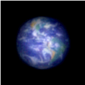
FIG. 23.: Simulated image of an Earth-like Planet detection (Courtesy: A. Labeyrie). An image of the Earth picture was convolved with the spread function from 150 point apertures, arrayed in 3 circles; it was multiplied by the hyper-telescope envelope, i.e. the spread function of the sub-pupils as well, and then pushed somewhat the contrast to attenuate the diffractive halo (Labeyrie, 2000).

VIII CONCLUSIONS

Earth-bound astronomical observations are strongly affected by atmospheric turbulence that set severe limits on the angular resolution, which in optical domain, is rarely better than $\sim$ 0.5^′′. A basic understanding of interference phenomenon is of paramount importance to other branches of physics and engineering as well. In recent years, a wide variety of applications of speckle patterns has been found in many areas. Though the statistical properties of the speckle pattern is complicated, a detailed analysis of this pattern is useful in information processing.

Image-processing is a very important subject. A second-order moment (power spectrum) analysis provides only the modulus of the object FT, whereas a third-order moment (bispectrum) analysis yields the phase allowing the object to be fully reconstructed. A more recent attempt to go beyond the third order, e.g., fourth-order moment (trispectrum), illustrates its utility in finding optimal quadratic statistics through the weak gravitational lensing effect (Hu, 2001). This algorithm provides a far more sensitive test than the bispectrum for some possible sources of non-Gaussianity (Kunz et al., 2001), however, its implementation in optical imaging is a difficult computational task. Deconvolution method is an important topic as well. It applies to imaging in general which covers methods spanning from simple linear deconvolution algorithms to complex non-linear algorithms.

In astronomy, the field of research that has probably benefited the most from high angular resolution techniques using single telescopes, and will still benefit in the future, is undoubtedly the origin and evolution of stellar systems. This evolution starts with star formation, including multiplicity, and ends with the mass loss process which recycles heavier elements into the interstellar medium. Large-scale star formation provides coupling between small-scale and large-scale processes. Stellar chemical evolution or nucleo-synthesis that is a result of star formation activity further influences evolutionary process. High resolution observations are fruitful for the detection of proto-planetary disks and possibly planets (either astrometrically, through their influence on the disk, or even directly). The technique is also being applied to studies of starburst and Seyfert galaxies, AGNs, and quasars. Studies of the morphology of stellar atmospheres, the circumstellar environment of nova or supernova, YPN, long period variables (LPV), rapid variability of AGNs etc. are also essential.

In spite of the limited capability of retrieving fully diffraction-limited images of the objects, AO systems are now offered to users of large telescopes. AO observations have contributed to the study of the solar system, and added to the results of space borne instruments, for examples, monitoring of the volcanic activity on Io or of the cloud cover on Neptune, the detection of Neptune’s dark satellites and arcs, and the ongoing discovery of companions to asteroids etc.; they are now greatly contributing to the study of the Sun itself as well (Antoshkin et al. 2000, Rimmele, 2000). Combination of AO systems with speckle imaging may enhance the results (Dayton et al. 1998). By the end of the next decade (post 2010), observations using the AO system on a new generation telescope like OWL, will revolutionize the mapping of ultra-faint objects like blazars that exhibit the most rapid and the largest amplitude variations of all AGN (Ulrich et al. 1997), extra-solar planets etc.; certain aspects of galactic evolution like chemical evolution in the Virgo cluster of galaxies can be studied as well.

A host of basic problems needs a very high angular resolution for their solution. Among others, an important fundamental problem that can be addressed with the interferometry and AO is the origin and evolution of galaxies. The upcoming large facilities with phased arrays of multiple 8-10 m sub-apertures will provide larger collecting areas and higher spatial resolution simultaneously than the current interferometers. These instruments fitted with complete AO systems would be able to provide imaging and morphological informations on the faint extragalactic sources such as, galactic centers in the young universe, deep fields, and host galaxies. Measurement of such objects may be made feasible by the instruments with a fairly complete $u,v$ coverage and large field of view. The derivations of motions and parallaxes of galactic centers seem to be feasible with phase reference techniques. Origin of faint structures close to non-obscured central sources can also be studied in detail with interferometric polarization measurement.

The capabilities of the proposed large arrays offer a revolution in the study of compact astronomical sources from the solar neighborhood to cosmological distances. The aim ranges from detecting other planetary systems to imaging the black hole driven central engines of quasars and active galaxies; gamma-ray bursters may be the other candidate. Another important scientific objective is the recording of spectra to derive velocity and to determine black hole masses as a function of redshift. At the beginning of the present millennium, several such arrays will be in operation both on the ground as well as in space. Space-borne interferometers are currently planned to detect planets either astrometrically (SIM) or directly (TPF). Projects like DARWIN and other ambitious imaging instruments may also come to function.

REFERENCES

- [1] Ables J. G., 1974, Astron. Astrophys. Suppl., 15, 383.
- [2] Aime C., 2000, J. Opt. A: Pure & Appl. Opt., 2, 411.
- [3] Akeson R., M. Swain, and M. Colavita, 2000, SPIE, 4006, 321.
- [4] Anderson J. A., 1920, Astrophys. J., 51, 263.
- [5] Angel J. R. P., 1994, Nature, 368, 203.
- [6] Angel J. R. P., 2001, Nature, 409, 427.
- [7] Angel J. R., and N. J. Woolf, 1997, Astrophy. J., 475, 373.
- [8] Antoshkin L. V. et al., 2000, SPIE, 4007, 232.
- [9] Aretxaga I., D. Mignant, J. Melnick, R. Terlevich, and B. Boyle, 1998, Mon. Not. R. Astron. Soc., 298, L13.
- [10] Armstrong J. T., C. A. Hummel, and D. Mozurkewich, 1992, Proc. ESO-NOAO conf. eds., J. M. Beckers & F. Merkle, ESO, Germany, 673.
- [11] Armstrong J. et al., 1998, Astrophys. J., 496, 550.
- [12] Arnold L., A. Labeyrie, and D. Mourard, 1996, Adv. Space Res. 18, 1148.
- [13] Ayers G. R., and J. C. Dainty, 1988, Opt. Lett., 13, 457.
- [14] Baba N., S. Kuwamura, N. Miura, and Y. Norimoto, 1994, Astrophys. J., 431, L111.
- [15] Baba N., S. Kuwamura, and Y. Norimoto, 1994, Appl. Opt., 33, 6662.
- [16] Baba N., H. Tomita, and N. Miura, 1994, Appl. Opt., 33, 4428.
- [17] Babcock H. W., 1953, Pub. Astron. Soc. Pac, 65, 229.
- [18] Babcock H. W., 1990, Science,249, 253.
- [19] Bagnuolo Jr. W. G., B. D. Mason, D. J. Barry, W. I. Hartkopf, and H. A. McAlister, 1992, Astron. J., 103, 1399.
- [20] Baldwin J. et al., 1996, Astron. Astrophys., 306, L13.
- [21] Baldwin J., R. Boysen, C. Haniff, P. Lawson, C. Mackay, J. Rogers, D. St-Jacques, P. Warner, D. Wilson, and J. Young, 1998, SPIE., 3350, 736.
- [22] Baldwin J. E., C. A. Haniff, C. D. Mackay, and P. J. Warner, 1986, Nature, 320, 595.
- [23] Baldwin J., R. Tubbs, G. Cox, C. Mackay, R. Wilson, and M. Andersen, 2001, Astron. Astrophys., 368, L1.
- [24] Baldwin J. E., and P. J. Warner, 1978, Mon. Not. R. Astron. Soc., 182, 411.
- [25] Balick B., 1987, Astron. J., 94, 671.
- [26] Barlow M. J., B. L. Morgan, C. Standley, and H. Vine, 1986, Mon. Not. R. Astron. Soc., 223, 151.
- [27] Barnaby D., E. Spillar, J. Christou, and J. Drummond, 2000, Astron. J., 119, 378.
- [28] Bates R., and M. McDonnell, 1986, ‘Image Restoration and Reconstruction’, Oxford Eng. Sc., Clarendon Press.
- [29] Beckers J. M., 1982, Opt. Acta., 29, 361.
- [30] Bedding T. R., D. Minniti, F. Courbin, and B. Sams, 1997, Astron. Astrophys., 326, 936.
- [31] Bedding T., A. Zijlstra, O. Von der Lühe, J. Robertson, R. Marson, J. Barton, and B. Carter, 1997, Mon. Not. R. Astron. Soc., 286, 957.
- [32] Beichman C., 1998, SPIE, 3350, 719.
- [33] Benson J., D. Mozurkewich, and S. Jefferies, 1998, SPIE, 3350, 493.
- [34] Berger J., P. Haguenauer, P. Kern, K. Perraut, F. Malbet, I. Schanen, M. Severi, R. Millan-Gabet, and W. Traub, 2001, Astron. Astrophys., 376, L31.
- [35] Berio P., D. Mourard, D. Bonneau, O. Chesneau, P. Stee, N. Thureau, and F. Vakili, 1999, J. Opt. Soc. Am. A., 16, 872.
- [36] Berio P., P. Stee, F. Vakili, D. Mourard, D. Bonneau, O. Chesneau, N. Thureau, D. Le Mignant, and R. Hirata, 1999, Astron. Astrophys., 345, 203.
- [37] Bester M., W. C. Danchi, C. G. Degiacomi, and C. H. Townes, 1991, Astrophys. J., 367, L27.
- [38] Beuzit J. et al., 2001, astro-ph/0106277.
- [39] Blazit A., 1986, SPIE, 702, 259.
- [40] Blöcker T., Y. Balega, K. -H. Hofmann, and G, Weigelt, 2001, Astron. Astrophys. (to appear).
- [41] Blum R., D. Schaerer, A. Pasquali, M. Heydari-Malayeri, P. Conti, and W. Schmutz, 2001, Astron. J., (to appear).
- [42] Boccaletti A., 2001, Private communication.
- [43] Boccaletti A., C. Moutou, D. Mouillet, A. Lagrange, and J. Augereau, 2001, Astron. Astrophys., 367, 371.
- [44] Boccaletti A., P. Riaud, C. Moutou, and A. Labeyrie, 2000, Icarus, 145, 628.
- [45] Boden A. et al., 1999, Astrophys. J., 515, 356.
- [46] Bonneau D., and R. Foy, 1980, Astron. Astrophys., 92, L1.
- [47] Bonneau D., and A. Labeyrie, 1973, Astrophys. J, 181, L1.
- [48] Born M., and E. Wolf, 1984, Principles of Optics, Pergamon Press.
- [49] Bouvier J., F. Rigaut, and D. Nadeau, 1997, Astron. Astrophys., 323, 139.
- [50] Bracewell R. N., 1978, Nature, 274, 780.
- [51] Brandl B., B. J. Sams, F. Bertoldi, A. Eckart, R. Genzel, S. Drapatz, R. Hofmann, M. Lowe, and A. Quirrenbach, 1996, Astrophys. J., 466, 254.
- [52] Brandner W., J. Bouvier, E. Grebel, E. Tessier, D. de Winter, and J. L. Beuzit, 1995, Astron. Astrophys., 298, 816.
- [53] Briggs D. S., 1995, Ph. D. Thesis, New Mexico Institute of Mining and Technology.
- [54] Bruns D., T. Barnett, and D. Sandler, 1997, SPIE., 2871, 890.
- [55] Burge J. H., B. Cuerdem, and J. R. P. Angel, 2000, SPIE, 4013, 640.
- [56] Burns D. et al., 1997, Mon. Not. R. Astron. Soc., 290, L11.
- [57] Burns D. et al., 1998, Mon. Not. R. Astron. Soc., 297, 467.
- [58] Butler R., and G. Marcy, 1996, Astrophys. J, 464, L153.
- [59] Cadot O., Y. Couder, A. Daerr, S. Douady, and A. Tsinocber, 1997, Phys. Rev., 56, 427.
- [60] Callados M., and M. Vàzquez, 1987, Astron. Astrophys., 180, 223.
- [61] Carleton N. et al., 1994, SPIE, 2200, 152.
- [62] Cassinelli J., J. Mathis, and B. Savage, 1981, Science, 212, 1497.
- [63] Charbonneau D., T. Brown, R. Noyes, and R. Gilfiland, 2001, Astrophys. J., (to appear).
- [64] Ciardi D., G. van Belle, R. Akeson, R. Thompson, E. A. Lada, and S. Howell, 2001, Astrophys. J. (to appear).
- [65] Clampin M., J. Croker, F. Paresce, and M. Rafal, 1988, Rev. Sci. Instru., 59, 1269.
- [66] Clampin M., A. Nota, D. A. Golimowski, C. Leitherer, and A. Ferrari, 1993, Astrophys. J., 410, L35.
- [67] Close L., F. Roddier, J. Hora, J. Graves, M. Northcott, C. Roddier, W. Hoffman, A. Doyal, G. Fazio, and L. Deutsch, 1997, Astrophys. J., 489, 210.
- [68] Colavita M., 1999, Pub. Astron. Soc. Pac., 111, 111.
- [69] Colavita M. et al., 1998, SPIE, 3350, 776.
- [70] Colavita M. et al., 1999, Astron. J., 117, 505.
- [71] Conan J. -M., L. M. Mugnier, T. Fusco, V. Michau, and G. Rousset, 1998, Appl. Opt., 37, 4614.
- [72] Conan R., A. Ziad, J. Borgnino, F. Martin, and A. Tokovinin, 2000, SPIE, 4006, 963.
- [73] Cooper D., D. Bui, R. Bailey, L. Kozlowski, and K. Vural, 1993, SPIE, 1946, 170.
- [74] Cornwell T. J., and P. N. Wilkinson, 1981, Mon. Not. R. Astron. Soc., 196, 1067.
- [75] Coudé du Foresto V., G. Perrin, and M. Boccas, 1995, Astron. Astrophys., 293, 278.
- [76] Coulman C. E., 1974, Solar Phys., 34, 491.
- [77] Coulman C. E., 1985, Annu. Rev. Astron. Astrophys., 23, 19.
- [78] Currie D., K. Kissel, E. Shaya, P. Avizonis, D. Dowling, and D. Bonnacini, 1996, The Messenger, no. 86, 31.
- [79] Danchi W. C., M. Bester, C. Degiacomi, I. Greenhill, and C. Townes, 1994, Astron. J., 107, 1469.
- [80] Danchi W. C., P. G. Tuthill, and J. D. Monnier, 2001, Astrophys. J. (to appear).
- [81] Dantowitz R., S. Teare, and M. Kozubal, 2000, Astron. J., 119, 2455.
- [82] Davidge T. J., F. Rigaut, R. Doyon, and D. Crampton, 1997, Astron. J., 113, 2094.
- [83] Davidge T. J., D. A. Simons, F. Rigaut, R. Doyon, E. E. Becklin, and D. Crampton, 1997, Astron. J., 114, 2586.
- [84] Davis J., and W. J. Tango, 1996, Pub. Astron. Soc. Pac., 108, 456.
- [85] Davis J., W. Tango, A. Booth, and J. O’Byrne, 1998, SPIE, 3350, 726.
- [86] Davis J., W. Tango, A. Booth, T. ten Brummelaar, R. Minard, and S. Owens, 1999a, Mon. Not. R. Astron. Soc., 303, 773.
- [87] Davis J., W. J. Tango, A. J. Booth, E. D. Thorvaldson, and J. Giovannis, 1999b Mon. Not. R. Astron. Soc., 303, 783.
- [88] Dayton D., S. Sandven, J. Gonglewski, S. Rogers, S. McDermott, and S. Browne, 1998, SPIE, 3353, 139.
- [89] Dejonghe J., L. Arnold, O. Lardière, J. -P Berger, C. Cazalé, S. Dutertre, D. Kohler, and D. Vernet, 1998, SPIE, 3352, 603.
- [90] Denker C., 1998, Solar Phys., 81, 108.
- [91] Derie F., M. Ferrai, E. Brunetto, M. Duchateau, R. Amestica, and P. Aniol, 2000, SPIE, 4006, 99.
- [92] DiBenedetto G. P., and Y. Rabbia, 1987, Astron. Astrophys., 188, 114.
- [93] Diericks P., and R. Gilmozzi, 1999, Proc. ‘Extremely Large Telescopes’, eds., T. Andersen, A. Ardeberg, and R. Gilmozzi, 43.
- [94] Drummond J., A. Eckart, and E. Hege, 1988, Icarus, 73, 1.
- [95] Dyck H., J. Benson, and S. Ridgway, 1993, Pub. Astron. Soc. Pac, 105, 610.
- [96] Dyck H., G. van Belle, and J. Benson, 1996, Astron. J., 112, 294.
- [97] Ebstein S., N. P. Carleton, and C. Papaliolios, 1989, Astrophys. J, 336, 103.
- [98] Eke V., 2001, Mon. Not. R. Astron. Soc., 320, 106.
- [99] Elias N. M., 2001, Astrophys. J., 549, 647.
- [100] Falcke H., K. Davidson, K. -H. Hofmann, and G. Weigelt, 1996, Astron. Astrophys. 306, L17.
- [101] Faucherre M., D. Bonneau, L. Koechlin, and F. Vakili, 1983, Astron. Astrophys. 120, 263.
- [102] Fienup J. R., 1978, Opt. Lett., 3, 27.
- [103] Fischer O., B. Stecklum, and C. Leinert, 1998, Astron. Astrophys., 334, 969.
- [104] Fizeau H., 1868, C. R. Acad. Sci. Paris, 66, 934.
- [105] Fomalont E. B., and M. C. H. Wright, 1974, in Galactic and Extra-galactic Radio Astronomy, eds., G. L. Verschuur, and K. I. Kellerman, 256.
- [106] Foy R., D. Bonneau, and A. Blazit, 1985, Astron. Astrophys., 149, L13.
- [107] Foy R., and A. Labeyrie, 1985, Astron. Astrophys., 152, L29.
- [108] Fried D. L., 1966, J. Opt. Soc. Am., 56, 1372.
- [109] Fugate R. et al., 1994, J. Opt. Soc. Am. A., 11, 310.
- [110] Gauger A., Y. Y. Balega, P. Irrgang, R. Osterbart, and G. Weigelt, 1999, Astron. Astrophys., 346, 505.
- [111] Gay J., and D. Mekarnia, 1988, Proc. ESO-NOAO conf. ed., F. Merkle, ESO, FRG, 811.
- [112] Gerchberg R. W., and W. O. Saxton, 1972, Optik, 35, 237.
- [113] Gies R., B. Mason, W. Bagnuolo, M. Haula, W. I. Hartkopf, H. McAlister, M. Thaller, W. McKibben, and L. Penny, 1997, Astrophys. J., 475, L49.
- [114] Glindemann A., 1997, Pub. Astron. Soc. Pac, 109, 682.
- [115] Glindemann A., R. G. Lane, and J. C. Dainty, 1991, Proc. ‘Digital Signal Processing’, eds., V. Cappellini & A. G. Constantinides, 59.
- [116] Glindemann A., and F. Paresce, 2001, http://www.eso.org/outreach.
- [117] Golimowski D. A., T. Nakajima, S. R. Kulkarni, and B. R. Oppenheimer, 1995, Astrophys. J, 444, L101.
- [118] Gonsalves S. A., 1982, Opt. Eng., 21, 829.
- [119] Goodman J. W., 1975, ‘Laser Speckle and Related Phenomena’, ed., J. C. Dainty, Springer-Verlag, Berlin, 9.
- [120] Goodman J. W., 1985, ‘Statistical Optics’, Wiley, N. Y.
- [121] Gorham P. W., 1998, SPIE, 3350, 116.
- [122] Gorham P., W. Folkner, and G. Blackwood, 1999, ASP conf., 194, eds. S. Unwin, and R. Stachnik, ISBN: 1-58381-020-X, 359.
- [123] Greenwood D. P., 1977, J. Opt. Soc. Am., 67, 390.
- [124] Grieger F., F. Fleischman, and G. Weigelt, 1988, Proc. ESO-NOAO conf. ed. F. Merkle, ESO, FRG, 225.
- [125] Haguenauer P., M. Sevei, I. Schanen-Duport, K. Rousselet-Perraut, J. Berger, Y. Duchéne, M. Lacolle, P. Kern, F. Melbet, and P. Benech, 2000, SPIE, 4006, 1107.
- [126] Hajian A. et al., 1998, Astrophys. J., 496, 484.
- [127] Hale D., M. Bester, W. Danchi, W. Fitelson, S. Hoss, E. Lipman, J. Monnier, P. Tuthill, and C. Townes, 2000, Astrohys, J., 537, 998.
- [128] Hale D. et al., 1997, Astrophys. J., 490, 826.
- [129] Hanbury Brown R., 1974, ‘The Intensity Interferometry, its Applications to Astronomy’, Taylor & Francis, London.
- [130] Hanbury Brown R., and R. Twiss, 1958, Proc. Roy. Soc. A, 248, 222.
- [131] Hanbury Brown R., R. C. Jennison, and M. K. Das Gupta, 1952, Nature, 170, 1061.
- [132] Haniff C., M. Scholz, and P. Tuthill, 1995, Mon. Not. R. Astron. Soc., 276, 640.
- [133] Harmanec P. et al., 1996, Astron. Astrophys., 312, 879.
- [134] Hartkopf W. I., H. A. McAlister, and B. D. Mason, 1997, CHARA Contrib. No. 4, ‘Third Catalog of Interferometric Measurements of Binary Stars’, W.I.
- [135] Hartley M., B. Mcinnes, and F. Smith, 1981, Q. J. Astr. Soc., 22, 272.
- [136] Harvey J. W., 1972, Nature, 235, 90.
- [137] Harvey J. W., and J. B. Breckinridge, 1973, Astrophys. J., 182, L137.
- [138] Hawley S. A., and J. S. Miller, 1977, Astrophys. J, 212, 94.
- [139] Hege E., E. Hubbard, P. Strittmatter, and S. Worden, 1981, Astrophys. J., 248, 1.
- [140] Hestroffer D., 1997, Astron. Astrophys., 327, 199.
- [141] Heydari M., and J. Beuzit, 1994, Astron. Astrophys., 287, L17.
- [142] Hickson P., 2001, Private communication.
- [143] Hill J. M., 2000, SPIE, 4004, 36.
- [144] Hinz P., R. Angel, W. Hoffmann, D. Mccarthy, P. Mcguire, M. Cheselka, J. Hora, and N. Woolf, 1998, Nature, 395, 251.
- [145] Hinz P., W. Hoffmann, and J. Hora, 2001, Astrophys. J. Lett. (to appear).
- [146] The Hipparcos Catalogue, 1997, ESA, SP-1200.
- [147] Hofmann K. -H., W. Seggewiss, and G. Weigelt, 1995, Astron. Astrophys., 300, 403.
- [148] Högbom J., 1974, Astron. Astrophys. Suppl., 15, 417.
- [149] Hu W., 2001, astro-ph/0105117
- [150] Hummel C., D. Mozurkevich, J. Armstrong, A. Hajian, N. Elias, and D. Hutter, 1998, Astron. J., 116, 2536.
- [151] Hutchings J., D. Crampton, S. Morris, D. Durand, and E. Steinbring, 1999, Astron. J., 117, 1109.
- [152] Hutchings J., D. Crampton, S. Morris, and E. Steinbring, 1998, Pub. Astron. Soc. Pac, 110, 374.
- [153] Hutchings J., S. Morris, and D. Crampton, 2001, Astron. J., 121, 80.
- [154] Ishimaru A., 1978, ‘Wave Propagation and Scattering in Random Media’, Academic Press, N. Y.
- [155] Jefferies S., and J. Christou, 1993, Astrophys. J, 415, 862.
- [156] Jennison R. C., 1958, Mon. Not. R. Astron. Soc., 118, 276.
- [157] Karovska M., L. Koechlin, P. Nisenson, C. Papaliolios, and C. Standley, 1989, Astrophys. J, 340, 435.
- [158] Kenworthy M. et al., 2001, Astrophys. J. Lett. (to appear).
- [159] Kervella P., V. Coudé du Foresto, G. Perrin, M. Schöller, W. Traub, and M. Lacasse, 2001, Astron. Astrophys., 367, 876.
- [160] Knox K., and B. Thompson, 1974, Astrophys. J, 193, L45.
- [161] Koechlin L., P. R. Lawson, D. Mourard, A. Blazit, D. Bonneau, F. Morand, P. Stee, I. Tallon-Bosc, and F. Vakili, 1996, Appl. Opt., 35, 3002.
- [162] Kolmogorov A., 1941a, in ‘Turbulence’, eds., S. K. Friedlander & L. Topper, 1961, Wiley-Interscience, N. Y., 151.
- [163] Kolmogorov A., 1941b, in ‘Turbulence’, eds., S. K. Friedlander & L. Topper, 1961, Wiley-Interscience, N. Y., 156.
- [164] Kolmogorov A., 1941c, in ‘Turbulence’, eds., S. K. Friedlander & L. Topper, 1961, Wiley-Interscience, N. Y., 159.
- [165] Korff D., 1973, J. Opt. Soc. Am., 63, 971.
- [166] Kunz M., A. Banday, P. Castro, P. Ferreira, and K. Górski, 2001, Astrophys. J. Lett., (to appear).
- [167] Labeyrie A., 1970, Astron. Astrophys., 6, 85.
- [168] Labeyrie A., 1975, Astrophys. J, 196, L71.
- [169] Labeyrie A., 1995, Astron. Astrophys., 298, 544.
- [170] Labeyrie A., 1996, Astron. Astrophys. Suppl., 118, 517.
- [171] Labeyrie A., 1998, SPIE, 3350, 960.
- [172] Labeyrie A., 1999a, ASP Conf., 194, eds. S. Unwin, and R. Stachnik, 350.
- [173] Labeyrie A., 1999b, Science, 285, 1864.
- [174] Labeyrie A., 2000, Private communication.
- [175] Labeyrie A., 2001, Private communication.
- [176] Labeyrie A., L. Koechlin, D. Bonneau, A. Blazit, and R. Foy, 1977, Astrophys. J., 218, L75.
- [177] Labeyrie A., G. Lamaitre, and L. Koechlin, 1986, SPIE, 628, 323.
- [178] Labeyrie A., G. Schumacher, M. Dugué, C. Thom, P. Bourlon, F. Foy, D. Bonneau, and R. Foy, 1986, Astron. Astrophys., 162, 359.
- [179] Lai O., D. Rouan, F. Rigaut, R. Arsenault, and E. Gendron, 1998, Astron. Astrophys., 334, 783.
- [180] Lai O., D. Rouan, F. Rigaut, F. Doyon, and F. Lacombe, 1999, Astron. Astrophys., 351, 834.
- [181] Lane B., M. Kuchner, A. Boden, M. Crooch-Eakman, and S. R. Kulkarni, 2000, Nature, 407, 485.
- [182] Lannes A., E. Anterrieu, and K. Bouyoucef, 1994, J. Mod. Opt., 41, 1537.
- [183] Lawson P. R., 1994, Pub. Astron. Soc. Pac., 106, 917.
- [184] Lawson P. R., 1995, J. Opt. Soc. Am A., 12, 306.
- [185] Lawson P., J. Baldwin, P. Warner, R. Boysen, C. Haniff, J. Rogers, D. Saint-Jacques, D. Wilson, and J. Young, 1998, SPIE, 3350, 753.
- [186] Lawson P., M. Colavita, P. Dumont, and B. Lane, 2000, SPIE, 4006, 397.
- [187] Ledoux C., B. Théodore, P. Petitjean, M. N. Bremer, G. F. Lewis, R. A. Ibata, M. J. Irwin, and E. J. Totten, 1998, Astron. Astrophys., 339, L77.
- [188] Lee J., B. Bigelow, D. Walker, A. Doel, and R. Bingham, 2000, Pub. Astron. Soc. Pac, 112, 97.
- [189] Lefèvre H. C., 1980, Electron. Lett., 16, 778.
- [190] Léger A., M. Pirre, and F. J. Marceau, 1993, Astron. Astrophys., 277, 309.
- [191] Liang J., D. R. Williams, and D. T. Miller, 1997, J. Opt. Soc. Am. A, 14, 2884.
- [192] Lindengren L., and M. A. C. Perryman, 1996, Astron. Astrophys. Suppl., 116, 579.
- [193] Linfield R., and P. Gorham, 1999, ASP Conf., 194, eds. S. Unwin, and R. Stachnik, ISBN: 1-58381-020-X, 224.
- [194] Lloyd-Hart M., 2000, Pub. Astron. Soc. Pac, 112, 264.
- [195] Lloyd-Hart M., J. R. Angel, T. Groesbeck, T. Martinez, B. Jacobsen, B. McLeod, D. McCarthy, E. Hooper, E. Hege, and D. Sandler, 1998, Astrophys. J., 493, 950.
- [196] Lipman E., M. Bester, W. Danchi, and C. Townes, 1998, SPIE, 3350, 933.
- [197] Liu Y. C., and A. W. Lohmann, 1973, Opt. Comm., 8, 372.
- [198] Lohmann A., G. Weigelt, and B. Wirnitzer, 1983, Appl. Opt., 22, 4028.
- [199] Lopez B. et al., 1997, Astrophys. J., 488, 807.
- [200] Lopez B., 1991, ‘Last Mission at La Silla, April 19 May 8, on the Measure of the Wavefront Evolution Velocity’, ESO Internal Report.
- [201] Lovelock J. E., 1965, Nature, 207, 568.
- [202] Lucy L., 1974, Astron. J., 79, 745.
- [203] Lynds C., S. Worden, and J. Harvey, 1976, Astrophys. J, 207, 174.
- [204] Machida Y. et al., 1998, SPIE, 3350, 202.
- [205] Macintosh B., C. Max, B. Zuckerman, E. Becklin, D. Kaisler, P. Lowrence, A. Weinberger, J. Christou, G. Schneider, and S. Acton, 2001, astro-ph/0106479.
- [206] Mackay C. D., R. N. Tubbs, R. Bell, D. Burt, P. Jerram, and I. Moody, 2001, SPIE, 4306, (in press).
- [207] Magain P., F. Courbin, and S. Sohy, 1998, Astrophys. J., 494, 472.
- [208] Malbet F. et al., 1998, Astrophys. J., 507, L149.
- [209] Marco O., T. Encrenaz, and E. Gendron, 1997, Planet Sp. Sci., 46, 547.
- [210] Márquez I., P. Petitjean, B. Théodore, M. Bremer, G. Monnet, and J. Beuzit, 2001, Astron. Astrophys., 371, 97.
- [211] Masciadri E., J. Vernin, and P. Bougeault, 1999, Astron. Astrophys. Suppl., 137, 203.
- [212] Mason B. D., 1996, Astron. J., 112, 2260.
- [213] Mason B., C. Martin, W. I. Hartkopf, D. Barry, M. Germain, G. Douglass, C. Worley, G. Wycoff, T. ten Brummelaar, and O. Franz, 1999, Astron. J., 117, 1890.
- [214] Mayor M., and D. Queloz, 1995, Nature, 378, 355.
- [215] McAlister H., W. Bagnuolo, T. ten Brummelaar, W. I. Hartkopf, M. Shure, L. Sturmann, N. Turner, and S. Ridgway, 1998, SPIE, 3350, 947.
- [216] Mendel L., and E. Wolf, 1995, ‘Optical Coherence and Quantum Optics’, Cambridge University Press, Cambridge.
- [217] Mennesson B., J. -M. Mariotti, V. Coudé du Foresto, G. Perrin, S. Ridgway, C. Ruilier, W. Traub, M. Lacasse, and G. Mazé, 1999, Astron. Astrophys., 346, 181.
- [218] Men’shchikov A., and T. Henning, 1997, Astron. Astrophys., 318, 879.
- [219] Michelson A. A., 1891, Nature, 45, 160.
- [220] Michelson A., and F. Pease, 1921, Astrophys. J, 53, 249.
- [221] Millan-Gabet R., P. Schloerb, and W. Traub, 2001, Astrophys. J., 546, 358.
- [222] Monnier J., W. Danchi, D. Hale, P. Tuthill, and C. Townes, 2000, Astrophys. J, 543, 868.
- [223] Monnier J., et al., 2001, AAS Meeting, 198, 63.02.
- [224] Monnier J., P. Tuthill, B. Lopez, P. Cruzalébes, W. Danchi, C. Haniff, 1999, Astrophys. J, 512, 351.
- [225] Morel S., 2000, Private communication.
- [226] Morel S., and L. Koechlin, 1998, SPIE, 3350, 257.
- [227] Morel S., W. Traub, J. Bregman, R. Mah, and C. Wilson, 2000, SPIE, 4006, 506.
- [228] Mouillet D., J. D. Larwood, J. C. Papaloizou, and A. M. Lagrange, 1997, Mon. Not. R. Astron. Soc., 292, 896.
- [229] Mourard D., D. Bonneau, L. Koechlin, A. Labeyrie, F. Morand, P. Stee, I. Tallon-Bosc, and F. Vakili, 1997, Astron. Astrophys., 317, 789.
- [230] Mourard D., I. Bosc, A. Labeyrie, L. Koechlin, and S. Saha, 1989, Nature, 342, 520.
- [231] Mozurkewich D., K. Johnston, R. Simon, D. Hutter, M. Colavita, M. Shao, and X. Pan, 1991, Astron. J., 101, 2207.
- [232] Nakajima T., 1994, Astrophys J., 425, 348.
- [233] Nakajima T., and D. Golimowski, 1995, Astron. J., 109, 1181.
- [234] Natta A., T. Prusti, R. Neri, D. Wooden, and V. Grinin, 2001, Astron. Astrophys., 371, 186.
- [235] Nelkin M., 2000, Am. J. Phys., 68, 310.
- [236] Nisenson P., and C. Papaliolios, 1999, Astrophys. J, 518, L29.
- [237] Nisenson P., C. Papaliolios, M. Karovska, and R. Noyes, 1987, Astrophys. J, 320, L15.
- [238] Nordgren T., J. Armstrong, M. Gierman, R. Hindsley, A. Hajian, J. Sudol, and C. Hummel, 2000, Astrophys. J., 543, 972.
- [239] Northcott M. J., G. R. Ayers, and J. C. Dainty, 1988, J. Opt. Soc. Am. A, 5, 986.
- [240] Nota A., C. Leitherer, M. Clampin, P. Greenfield, and D. A. Golimowski, 1992, Astron. J., 398, 621.
- [241] Nulsen P., P. Wood, P. Gillingham, M. Bessel, M. Dopita, and C. McCowage, 1990, Astrophys. J, 358, 266.
- [242] Osterbart R., Y. Balega, G. Weigelt, and N. Langer, 1996, Proc. IAU symp. 180, eds., H. Habing & G. Lamers, Kluwer Academic Pub. Netherlands, 362.
- [243] Padilla C., V. Karlov, L. Matson, K. Soosaar, and T. ten Brummelaar, 1998, SPIE, 3350, 1045.
- [244] Papaliolios C., M. Karovska, L. Koechlin, P. Nisenson, C. Standley, and S. Heathcote, 1989, Nature, 338, 565.
- [245] Papaliolios C., P. Nisenson, and S. Ebstein, 1985, Appl. Opt., 24, 287.
- [246] Pauls T., D. Mozurkewich, J. Armstrong, C. Hummel, J. Benson, and A. Hajian, 1998, SPIE, 3350, 467.
- [247] Paxman R., T. Schulz, and J. Fienup, 1992, J. Opt. Soc. Am., 9, 1072.
- [248] Paxman R., J. Seldin, M. Löfdahl, G. Scharmer, and C. Keller, 1996, Astrophys. J., 466, 1087.
- [249] Pedretti E., and A. Labeyrie, 1999, Astron. Astrophys. Suppl., 137, 543.
- [250] Pedretti E., A. Labeyrie, L. Arnold, N. Thureau, O. Lardiére, A. Boccaletti, and P. Riaud, 2000, Astron. Astrophys. Suppl., 147, 285.
- [251] Pehlemann E., K. -H Hofmann, and G. Weigelt, 1992, Astron. Astrophys., 256, 701.
- [252] Penny A., A. Léger, J. Mariotti, C. Schalinski, C. Eiora, R. Laurance, M. Fridlund, 1998, SPIE, 3350, 666.
- [253] Perrin G., 1997, Astron. Astrophys. Suppl., 121, 553.
- [254] Perrin G., V. Coudé du Foresto, S. Ridgway, J. -M. Marrioti, W. Traub, N. Carleton, M. Lacasse, 1998, Astron. Astrophys., 331, 619.
- [255] Perrin G., V. Coudé du Foresto, S. Ridgway, B. Mennesson, C. Ruilier, J. -M. Marrioti, W. Traub, and M. Lacasse, 1999, Astron. Astrophys., 345, 221.
- [256] Perryman M. A. C., 1998, Nature, 340, 111.
- [257] Poulet F., and B. Sicardy, 1996, Bull. Astr. Am. Soc., 28, 1124.
- [258] Pourbaix D., 2000, Astron. Astrophys. Suppl., 145, 215.
- [259] Prieur J., E. Oblak, P. Lampens, M. Kurpinska-Winiarska, E. Aristidi, L. Koechlin, and G. Ruymaekers, 2001, Astron. Astrophys., 367, 865.
- [260] Puetter R., and A. Yahil, 1999, astro-ph/9901063.
- [261] Quirrenbach A., 2001, Annu. Rev. Astron. Astrophys., 39, 353.
- [262] Quirrenbach A., D. Mozurkewich, D. Buscher, C. Hummel, and J. Armstrong, 1996, Astron. Astrophys., 312, 160.
- [263] Quirrenbach A., J. Roberts, K. Fidkowski, W. de Vries, and W. van Breugel, 2001, Astrophys. J. (to appear).
- [264] Rabbia Y., D. Mekarnia, and J. Gay, 1990, SPIE, 1341, 172.
- [265] Racine R., 1984, IAU Colloq. 79, eds., M. Ulrich & Kjär, 235.
- [266] Racine R., G. Herriot, and R. McClure, 1996, Proc. ‘Adaptive Optics’ ed., M. Cullum, ESO, Germany, 35.
- [267] Ragazzoni R., and D. Bonaccini, 1996, Proc. ‘Adaptive Optics’, ed., M. Cullum, 17.
- [268] Ragazzoni R., E. Marchetti, and G. Valente, 2000, Nature, 403, 54.
- [269] Reinheimer T., and G. Weigelt, 1987, Astron. Astrophys., 176, L17.
- [270] Richardson W. H., 1972, J. Opt. Soc. Am., 62, 55.
- [271] Ridgway S. T., and F. Roddier, 2000, SPIE, 4006, 940.
- [272] Rimmele T. R., 2000, SPIE, 4007, 218.
- [273] Robbe S., B. Sorrente, F. Cassaing, Y. Rabbia, and G. Rousset, 1997, Astron. Astrophys. Suppl. 125, 367.
- [274] Robertson N. A., 2000, Class. Quantum. Grav., 17, 19.
- [275] Roddier C., and F. Roddier, 1988, Proc. NATO-ASI workshop, eds., D. M. Alloin & J. -M. Mariotti, 221.
- [276] Roddier C., F. Roddier, M. J. Northcott, J. E. Graves, and K. Jim, 1996, Astrophys. J, 463, 326.
- [277] Roddier F., 1981, Progress in Optics, XIX, 281.
- [278] Roddier F., 1988, Phys. Rep., 170, 97.
- [279] Roddier F., 1999, ‘Adaptive Optics in Astronomy’, ed., F. Roddier, Cambridge Univ. Press.
- [280] Roddier F., C. Roddier, A. Brahic, C. Dumas, J. Graves, M. Northcott, and T. Owen, 1997, Planet Sp. Sci., 45, 1031.
- [281] Roddier F., C. Roddier, J. E. Graves, and M. J. Northcott, 1995, Astrophys. J, 443, 249.
- [282] Roggemann M. C., B. M. Welsh, and R. Q. Fugate, 1997, Rev. Modern Phys., 69, 437.
- [283] Rouan D., D. Field, J. -L. Lemaire, O. Lai, G. P. Forëts, E. Falgarone, and J. -M. Deltorn, 1997, Mon. Not. R. Astron. Soc., 284, 395.
- [284] Rouan D., P. Riaud, A. Boccaletti, Y. Clénet, and A. Labeyrie, 2000, Pub. Astron. Soc. Pac., 112, 1479.
- [285] Rouan D., F. Rigaut, D. Alloin, R. Doyon, O. Lai, D. Crampton, E. Gendron, and R. Arsenault, 1998, Astron. Astrophys., 339, 687.
- [286] Rousset G., 1999, ‘Adaptive Optics in Astronomy’, ed., F. Roddier, Cambridge Univ. Press, 91.
- [287] Rousset G., J. C. Fontanella, P. Kem, P. Gigan, F. Rigaut, P. Léna, P. Boyer, P. Jagourel, J. P. Gaffard, and F. Merkle, 1990, Astron. Astrophys., 230, L29.
- [288] Rousselet-Perraut K., F. Vakili, and D. Mourard, 1996, Opt. Eng., 35, 2943.
- [289] Ryan S., and P. Wood, 1995, Pub. Astron. Soc. Austr., 12, 89.
- [290] Saha S. K., 1999, Bull. Astron. Soc. Ind., 27, 443.
- [291] Saha S. K., and V. Chinnappan, 1999, Bull. Astron. Soc. Ind., 27, 327.
- [292] Saha S. K., and D. Maitra, 2001, Ind. J. Phys., 75B, 391.
- [293] Saha S. K., and S. Morel, 2000, Bull. Astron. Soc. Ind., 28, 175.
- [294] Saha S. K., R. Rajamohan, P. Vivekananda Rao, G. Som Sunder, R. Swaminathan, and B. Lokanadham, 1997, Bull. Astron. Soc. Ind., 25, 563.
- [295] Saha S. K., R. Sridharan, and K. Sankarasubramanian, 1999, ‘Speckle image reconstruction of binary stars’, Presented at XIX ASI meeting, Bangalore.
- [296] Saha S. K., and P. Venkatakrishnan, 1997, Bull. Astron. Soc. Ind., 25, 329.
- [297] Sams B. J., K. Schuster, and B. Brandl, 1996, Astrophys. J., 459, 491.
- [298] Sato K. et al., 1998, SPIE, 3350, 212.
- [299] Schertl D., K. -H. Hofmann, W. Seggewiss, and G. Weigelt, 1996, Astron. Astrophys., 302, 327.
- [300] Schöller M., W. Brandner, T. Lehmann, G. Weigelt, and H. Zinnecker, 1996, Astron. Astrophys., 315, 445.
- [301] Seldin J., R. Paxman, and C. Keller, 1996, SPIE., 2804, 166.
- [302] Seldin J., and R. Paxman, 1994, SPIE., 2302, 268.
- [303] Serabyn E., 2000, SPIE, 4006, 328.
- [304] Shannon C. J., 1949, Proc. IRE, 37, 10.
- [305] Shao M., and M. M. Colavita, 1992, Astron. Astrophys., 262, 353.
- [306] Shao M., and M. M. Colavita, 1994, Proc. IAU Symp. 158, eds., J. G. Robertson and W. J. Tango, 413.
- [307] Shao M., and D. Staelin, 1977, J. Opt. Soc. Am., 67, 81.
- [308] Shao M. et al., 1988, Astron. Astrophys., 193, 357.
- [309] Sicardy B., F. Roddier, C. Roddier, E. Perozzi, J. E. Graves, O. Guyon, and M. J. Northcott, 1999, Nature, 400, 731.
- [310] Simon M., L. Close, and T. Beck, 1999, Astron. J., 117, 1375.
- [311] Stee P., de Araújo, F. Vakili, D. Mourard, I. Arnold, D. Bonneau, F. Morand, and I. Tallon-Bosc, 1995, Astron. Astrophys., 300, 219.
- [312] Stee P., F. Vakili, D. Bonneau, and D. Mourard, 1998, Astron. Astrophys., 332, 268.
- [313] Tallon M., R. Foy, and A. Blazit, 1988, Proc. ESO Conf. ed., M. -H. Ulrich, ESO, FRG, 743.
- [314] Tango W. J., and R. Q. Twiss, 1980, Prog. Opt., 17, 239.
- [315] Tatarski V. I., 1967, ‘Wave Propagation in a Turbulent Medium’, Dover, New York.
- [316] Tatarski V. I., 1993, J. Opt. Soc. Am. A, 56, 1380.
- [317] Taylor G. L., 1921, in ‘Turbulence’, eds., S. K. Friedlander & L. Topper, 1961, Wiley-Interscience, New York, 1.
- [318] Thom C., P. Granes, and F. Vakili, 1986, Astron. Astrophys., 165, L13.
- [319] Thompson L. A., and C. S. Gardner, 1988, Nature, 328, 229.
- [320] Timothy J. G., 1993, SPIE., 1982, 4.
- [321] Torres G., R. Stefanik, and D. Latham, 1997, Astrophys. J, 485, 167.
- [322] Townes C. H., M. Bester, W. Danchi, D. Hale, J. Monnier, E. Lipman, A. Everett, P. Tuthill, M. Johnson, and D. Walters, 1998, SPIE, 3350, 908.
- [323] Traub W. A., 1986, Appl. Opt., 25, 528.
- [324] Traub W. A., 2000, Course notes on ‘Principles of long baseline interferometry’, ed., P. R. Lawson, 31.
- [325] Traub W. A. et al., 2000, SPIE, 4006, 715.
- [326] Traub W. A., R. Millam-Gabet, and M. Garcia, 1998, Bull. Astr. Am. Soc., 193, 52.06.
- [327] Troxel S. E., B. M. Welsh, and M. C. Roggemann, 1994, J. Opt. Soc. Am. A, 11, 2100.
- [328] Tuthill P., C. Haniff, and J. Baldwin, 1997, Mon. Not. R. Astron. Soc., 285, 529.
- [329] Tuthill P., C. Haniff, and J. Baldwin, 1999, Mon. Not. R. Astron. Soc., 306, 353.
- [330] Tuthill P. G., J. D. Monnier, and W. C. Danchi, 1999, Nature, 398, 487.
- [331] Tuthill P. G., J. D. Monnier, and W. C. Danchi, 2001, Nature, 409, 1012.
- [332] Tuthill P. G., J. D. Monnier, W. C. Danchi, and Wishnow, 2000, Pub. Astron. Soc. Pac., 116, 2536.
- [333] Ulrich M., L. Maraschi, and C. Urry, 1997, Annu. Rev. Astron. Astrophys., 35, 445.
- [334] Unwin S., S. Turyshev, and M. Shao, 1998, SPIE, 3350, 551.
- [335] Vakili F., D. Mourard, D. Bonneau, F. Morand, and P. Stee, 1997, Astron. Astrophys., 323, 183.
- [336] Vakili F., D. Mourard, P. Stee, D. Bonneau, P. Berio, O. Chesneau, N. Thureau, F. Morand, A. Labeyrie, and I. Tallon-Bosc, 1998, Astron. Astrophys., 335, 261.
- [337] van Belle G. et al., 1999, Astron. J., 117, 521.
- [338] van Belle G., D. Ciardi, R. Thompson, R. Akeson, and E. A. Lada, 2001, astro-ph/0106184.
- [339] van Belle G., H. Dyck, J. Benson, and M. Lacasse, 1996, Astron. J., 112, 2147.
- [340] van Belle G., H. Dyck, R. Thomson, J. Benson, and S. Kannappan, 1997, Astron. J., 114, 2150.
- [341] Von der Lühe O., 1984, J. Opt. Soc. Am. A, 1, 510.
- [342] Walkup J. F., and J. W. Goodman, 1973, J. Opt. Soc. Am, 63, 399.
- [343] Wallace J. et al., 1998, SPIE, 3350, 864.
- [344] Wehinger P. A., 2001, Private communication.
- [345] Weigelt G., 1977, Opt. Communication, 21, 55.
- [346] Weigelt G., and G. Bair, 1985, Astron. Astrophys., 150, L18.
- [347] Weigelt G., Y. Balega, T. Blöcker, A. Fleischer, R. Osterbart, and J. Winters, 1998, Astron. Astrophys., 333, L51.
- [348] Weigelt G., Y. Balega, K. -H. Hofmann, and M. Scholz, 1996, Astron. Astrophys., 316, L21.
- [349] Weigelt G., and J. Ebersberger, 1986, Astron. Astrophys., 163, L5.
- [350] Weinberger A., G. Neugebauer, and K. Matthews, 1999, Astron. J., 117, 2748.
- [351] Wilken V., C. R. de Boer, C. Denker, and F. Kneer, 1997, Astron. Astrophys., 325, 819.
- [352] Wilson R., J. Baldwin, D. Busher, and P. Warner, 1992, Mon. Not. R. Astron. Soc., 257, 369.
- [353] Wittkowski M., Y. Balega, T. Beckert, W. Duschi, K. Hofmann, and G. Weigelt, 1998, Astron. Astrophys., 329, L45.
- [354] Wittkowski M., Y. Balega, K. Hofmann, and G. Weigelt, 1999, Mitteilungen der Astronomischen Gesellschaft (AGM)., 15, 83.
- [355] Wittkowski M., C. Hummel, K. Johnston, D. Mozurkewich, A. Hajian, and N. White, 2001, Astron. Astrophys., 377, 981.
- [356] Wittkowski M., N. Langer, and G. Weigelt, 1998, Astron. Astrophys., 340, L39.
- [357] Wood P., M. Bessel, and M. Dopita, 1986, Astrophys. J, 311, 632.
- [358] Wood P., P. Nulsen, P. Gillingham, M. Bessel, M. Dopita, and C. McCowage, 1989, Astrophys. J, 339, 1073.
- [359] Worden S. P., C. R. Lynds, and J. W. Harvey, 1976, J. Opt. Soc. Am., 66, 1243.
- [360] Wyngaard J. C., Y. Izumi, and S. A. Collins, 1971, J. Opt. Soc. Am., 60, 1495.
- [361] Young A. T., 1974, Astrophys. J., 189, 587.
- [362] Young J. et al., 2000, Mon. Not. R. Astron. Soc., 315, 635.
- [363] Zago L., 1995, http://www.eso.org/gen-fac/pubs/astclim/lz-thesis/node4-html.