Angular momentum induced phase transition in spherical gravitational systems: N-body simulations

Abstract

The role of thermodynamics in the evolution of systems evolving under purely gravitational forces is not completely established. Both the infinite range and singularity in the Newtonian force law preclude the use of standard techniques. However, astronomical observations of globular clusters suggests that they may exist in distinct thermodynamic phases. Here, using dynamical simulation, we investigate a model gravitational system which exhibits a phase transition in the mean field limit. The system consists of rotating, concentric, mass shells of fixed angular momentum magnitude and shares identical equilibrium properties with a three dimensional point mass system satisfying the same condition. The mean field results show that a global entropy maximum exists for the model, and a first order phase transition takes place between ”quasi-uniform” and ”core-halo” states, in both the microcanonical and canonical ensembles. Here we investigate the evolution and, with time averaging, the equilibrium properties of the isolated system. Simulations were carried out in the transition region, at the critical point, and in each clearly defined thermodynamic phase, and striking differences were found in each case. We find full agreement with mean field theory when finite size scaling is accounted for. In addition, we find that (1) equilibration obeys power law behavior, (2) virialization, equilibration, and the decay of correlations in both position and time, are very slow in the transition region, suggesting the system is also spending time in the metastable phase, (3) there is strong evidence of long-lived, collective, oscillations in the supercritical region.

I Introduction

In contrast with ”normal” systems with short range interactions, the thermodynamics of self-gravitating systems is non-extensive and, because of the infinite range and singularity of the Newtonian potential, cannot be treated by standard methods. A partial remedy for these problems can be constructed by confining the system in a finite volume and either using a regularized Newtonian pair interaction potential, or considering the N-body system in the mean-field limit where it is possible to construct an analytic theory of $f(\mathbf{r},\mathbf{v})$ , the single particle density in position and velocity. The first mean-field formulations showed that (1) spherically symmetric density profiles represent the states of highest entropy and (2) a global entropy maximum does not exist Antonov (1985). It is always possible to increase the entropy by simultaneously increasing the central density and transferring mass to a diffuse ”halo” to control the value of the energy. This phenomenon, called gravothermal catastrophe in the literature, reflects the fact that an isolated and bounded gravitational system cannot be in equilibrium in the mean-field limit. Locally stable and unstable entropy extrema can exist, however, if the system’s energy is above a critical value Antonov (1985); Lynden-Bell and Wood (1968), and their stability has been investigated by several authors Padmanabhan (1989); Katz (1978, 1979).

In addition to the total energy, $E$, in the mean field limit the sum of squares of the angular momentum, $L_{2}=\lim\limits_{N->\infty}1/N\sum l_{i}^{2}$ , where $\mathbf{\ l}_{i}$ is the angular momentum of a system element, is also an integral of motion for a spherically symmetric gravitational system, Binney and Tremaine (1987) . If, along with the energy, this constraint is also included in MFT (mean field theory) the result is an anisotropic distribution in velocity. The result was first obtained by Eddington from a different route Eddington (1915). Until recently, this second integral has been ignored in investigations of thermodynamic stability in the mean field (Vlasov) limit, leaving open the possibility that a centrifugal barrier could prevent collapse and stabilize the system. In fact, we have recently shown that even its inclusion in MFT cannot resolve the gravothermal catastrophe, and it persists in both the generalized microcanonical ($E-L_{2}$) and canonical ($\beta-\gamma$) ensembles Klinko and Miller (2000). The extremal solutions have the form $f\propto\exp(-\beta\epsilon)\exp(-\gamma l^{2})$, which coincides with the well known anisotropic density fit models that have been applied to globular cluster observations with some success(e.g. King-Michie models) Gunn and Griffin (1979); Heggie and Meylan (1997).

In their seminal work on the gravothermal catastrophe, Lynden-Bell and Wood Lynden-Bell and Wood (1968) pointed out that in the absence of the short range singularity, the possibility existed for a gravitational system to exist in different thermodynamics phases. Using mean-field models with a regularized Newtonian potential which has been dissected to remove the singularity Kiessling (1989) or, equivalently, introducing repulsion at short-range by imposing a local equation of state in the mean field picture Aronson and Hansen (1972); Stahl et al. (1995); Padmanabhan (1989), it has been shown that a first order phase transition can occur in both the microcanonical (MCE) and canonical (CE) ensembles. Unfortunately, for finite $N$ systems, there are no exact microcanonical results available which allow the rigorous proof of a phase transition or catastrophe. However, in the canonical case, it has been rigorously proved that the system of gravitating point masses is in a collapsed state in equilibrium in the absence of regularization Kiessling (1989). Moreover, Monte-Carlo simulations for a regularized Newtonian potential confirm the gravitational phase transition in CE de Vega and Sánchez (2000) in large $N$ systems.

While mean field theories support the existence of phase transitions in gravitational systems, it is important to point out that there is no guarantee that these equilibrium states will be realized by dynamical evolution. In fact, there is no proof that the two operations of taking (1) the mean field limit, or (2) the infinite time average, commute Latora et al. (2001). Rather, simulations of the one dimensional self-gravitating system consisting of parallel mass sheets provide strong evidence to the contrary Mineau et al. (1990). As a consequence, the relation between maximum entropy solutions of the stationary mean field equation and the time average distribution functions resulting from N body simulation, or dynamical evolution in nature, has not been fully established. This is a deep question which will not be explored further here. Thus, although much is known concerning the ”equilibrium” properties in the mean field limit, the dynamical properties of gravitational phase transitions are not well known due to a lack of true N-body simulations, which are also important for explaining the evolution of stellar clusters, galaxies, etc.. At the present time the mean-field predictions of the gravitational phase transition have only been dynamically confirmed (in both MCE and CE) for the model system consisting of irrotational, concentric, mass shells Miller and Youngkins (1997a). In that model, the Newtonian singularity was screened by the introduction of an inner barrier which excluded mass from the system center.

The aim of this paper is to investigate and understand the dynamical features of gravitational phase transitions in N-body simulations for the model of a purely Newtonian system in which $l_{i}^{2}=l^{2}=L_{2}$ for each system element. We will refer to this system as the $l^{2}$ model. We will explicitly investigate a system of rotating, concentric, mass shells. In the mean field limit, this system shares important features, e.g. the equilibrium density and radial velocity distribution, with the more realistic system of point masses. Recently, with I. Prokhorenkov, we showed that the gravitational phase transition is present in both MCE and CE in certain regions of $l^{2}$ and we studied its properties using mean field theory Klinko et al. (2001). Moreover, we rigorously proved the existence of an upper bound for the entropy in the MCE (lower bound in the free energy in the CE) for $l^{2}\neq 0$ in the same work. It is important to understand that this model demonstrates the significance of the influence of angular momentum on the thermodynamics of self-gravitating systems, even if they are spherical. The generalized microcanonical ($E-L_{2}$) and canonical ($\beta-\gamma$) ensembles discussed earlier Klinko and Miller (2000)are appropriate for large $N$ spherical systems where angular momentum exchange occurs. While providing the most general mean field description Klinko and Miller (2000), $L_{2}$ is still not a sufficient constraint to resolve the gravothermal catastrophe. Clearly the culprit is angular momentum exchange, which is still permitted even if both energy and $L_{2}$ are fixed, and allows the transfer of mass to the system center. An open question is the possible existence of additional mechanisms for establishing a centrifugal barrier which prevents, or strongly inhibits, collapse in nature, e.g. in globular clusters or molecular clouds. This will be taken up in the final section.

In the following, first we briefly review the $l^{2}$ model, including the mean-field predictions, and discuss the main features of the N-body algorithm we designed for its dynamical simulation. Next we turn to the simulation results in a region of the $(E,l^{2})$ phase plane containing the microcanonical phase transition region. In each phase we compare the time-averaged equilibrium properties with the predictions of mean field theory resulting from our earlier investigation, and also touch on finite size effects. We then go on to study both equilibrium and dynamical features which cannot be predicted by mean field theory, such as the variance of fluctuations, and correlations in both time and position. In addition to the system behavior near the phase transition, we pay particular attention to the critical point, and the supercritical region. Finally we consider the surprising features exhibited by different stages of the relaxation process itself, and their dependence on energy, $l^{2}$, and population, and discuss the possible presence of collective modes.

Figure 1: Plot of the entropy extrema in the microcanonical ensemble for $l^{2}=5\times 10^{-5}$ in the mean-field limit. As we can see, in the transition region multiple solutions are present, and we marked the solutions for $E=2$ with labels 1, 2, and 3. Only phase 1 (quasi-uniform phase) is a global entropy maximum above the transition point ($E=1.9)$, while phase 2 (condensed phase) is locally stable, and phase 3 is a saddle point.

Figure 2: Density profiles of the three distinct phases labelled in Fig. 1 for $E=2$ in the transition region. Above the transition point only the quasi-uniform phase (phase 1) is globally stable, while the condensed phase (phase 2) is locally stable. The third entropy extremum (phase 3) is unstable.

Figure 3: The mean-field microcanonical phase diagram. The system can exist in 3 different types of phase depending on the energy and $l^{2}$, and we named these phases in analogy with normal systems. We also indicated the metastable regions which are important for understanding the dynamical behavior of the system near the transition point.

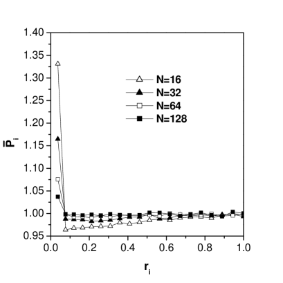
Figure 4: The time averaged relative populations $\bar{P}_{i}$ of relaxed systems in the high energy region at $E=4$ and $l^{2}=5\times 10^{-5}$ with $N_{bin}=20$. The bins were obtained from the equal-mass radii of the mean-field equilibrium density profile. We observe good convergence to the mean-field density profile with increasing $N$. As a result of finite size effects, the central density is higher than the mean-field density profile in the high energy region, and causes a reduction in the virial ratio.

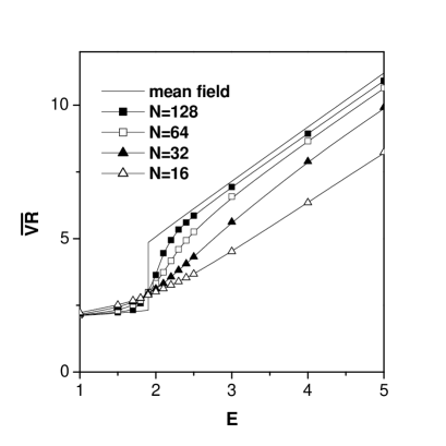
Figure 5: The averaged virial ratio $\overline{VR}$ for $56$ simulations for $N=16,32,64,128$ in and around the mean-field transition region. We also included the mean-field results for the globally stable states which show that the system undergoes a first order phase transition at $E=1.9$, where the virial ratio becomes discontinuous. The simulation results converge to the mean-field predictions with increasing $N$, but the transition point is shifted and the transition region is rounded, in good agreement with finite-size scaling.

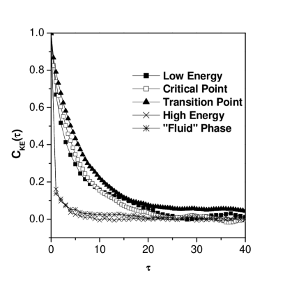
Figure 6: The time correlation function of the kinetic energy $C_{KE}\left(\tau\right)$ in 5 different phase regions for $N=64$, where $\tau$ is in units of $t_{dyn}$. In both the high energy ($E=4,l^{2}=5\times 10^{-5}$) and supercritical phase ($E=4,l^{2}=5\times 10^{-3}$), correlations are smaller, while in the low energy phase ($E=1.5,l^{2}=5\times 10^{-5}$), at the transition point ($E=1.9,l^{2}=5\times 10^{-5}$), and at the critical point ($E=1.052,l^{2}=1.1\times 10^{-4}$) relatively stronger correlations can be observed. Note that only the initial decay of the correlation functions follows an exponential behavior, then a long tail develops.

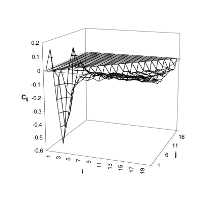
Figure 7: Position correlation matrix in relative bin populations $C_{ij}$, for $N_{bin}=20$ and $i>j$ in the low energy phase ($E=1,l^{2}=5\times 10^{-5},N=64$). The bin radii represent the equal-mass layers obtained from the mean-field density profile. Strong anti-correlation is present close to the high density central core region.

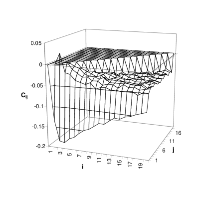
Figure 8: Position correlation matrix in relative bin populations $C_{ij}$, for $N_{bin}=20$ and $i>j$ in the phase transition region ($E=2,l^{2}=5\times 10^{-5},N=64$). The bin radii represent the equal-mass shells obtained from the mean-field density profile of phase 1 in Fig. 1. Strong anti-correlation is present between the center and the remainder of the system.

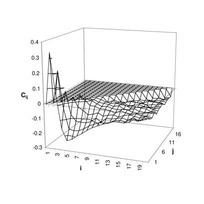
Figure 9: Position correlation matrix in relative populations $C_{ij}$, for $N_{bin}=20$ and $i>j$ near the critical point of the phase diagram ($E=1.052,l^{2}=1.1\times 10^{-4},N=64$). The bin radii represent the equal-mass shells obtained from the mean-field density profile. The behavior is similar to that of the low energy phase, although the anti-correlating region is wider. This reflects the fact that, at the critical point, the difference between the two distinct phases vanishes. This intermediate state still has a core-halo structure, but with a more extended core region.

Figure 10: Violent relaxation in the high energy phase ($E=4,l^{2}=5\times 10^{-5}$) in four simulations with $N=16,32,64,128$. In the figure $N$ is increasing from bottom to top. We observe that virialization is faster with increasing $N$. For $N=64,128$ the differences become marginal as we approach the mean-field limit.

Figure 11: Violent relaxation in the low energy phase ($E=1,l^{2}=5\times 10^{-5}$) at $N=16,32,64,128$ (from top to bottom in the figure). Here the virialization is also fast for larger values of $N$, and takes place on a much shorter time-scale than in the high energy phase. Note that for $N=64,128$, the system virializes in $100t_{dyn}$.

Figure 12: Violent relaxation in the phase transition region ($E=2,l^{2}=5\times 10^{-5}$) in four different simulations. From bottom to top $N=16,32,64,128$. Compared with the high and low energy phases, the relaxation is slower for larger $N$ as opposed to the process in the high and low energy phases. As we approach the mean-field limit, the phase transition becomes sharper and the increasing influence of the meatstable phase slows down the relaxation.

Figure 13: Plots of $\sigma_{r}^{2}$ vs. time which indicate the relaxation process in $\mu$ space for simulations with $N=16,32,64,128$ in the high energy phase ($E=4,l^{2}=5\times 10^{-5}$). In order to avoid statistical error while sampling the populations, we chose snapshot times $t_{s}=0.125,0.25,0.5,1$ for the corresponding values of $N$. For all $N$, the same power-law type of relaxation, $\sigma_{r}^{2}\propto 1/t$, can be observed.

Figure 14: Plots of $\sigma_{r}^{2}$ vs. time which indicate the relaxation process in $\mu$ space with simulations $N=16,32,64,128$ in the phase transition region ($E=2,l^{2}=5\times 10^{-5}$). In order to avoid statistical error during sampling the populations, we chose snapshot times $t_{s}=0.125,0.25,0.5,1$ for the corresponding $N$. The power-law behavior can still be observed, but large fluctuations start to take place with increasing $N$. As a result of the influence of the metastable phase, relaxation is slower for larger $N$ in this region.

Figure 15: Plots of $\sigma_{r}^{2}$ vs. time which indicate the process of relaxation in $\mu$ space for simulations with $N=16,32,64,128$ in the low energy phase ($E=1,l^{2}=5\times 10^{-5}$). In order to avoid statistical error during sampling the populations, we chose snapshot times $t_{s}=0.125,0.25,0.5,1$ for the corresponding values of $N$’s. In the high energy phase, we observe a similar power-law relaxation which also follows $\sigma_{r}^{2}\propto 1/t$.

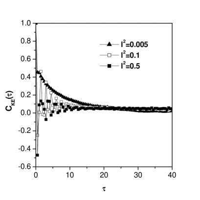
Figure 16: The time correlation of the kinetic energy $C_{KE}\left(\tau\right)$ versus time for three regions of the supercritical phase at the energy $E=0$. With increasing $l^{2}$, an oscillating part starts to sit on top of the correlation functions which suppresses the early exponential behavior, and a very long tail starts to develop.

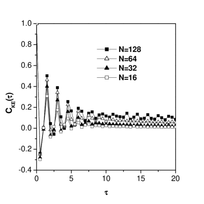
Figure 17: $N$ dependence of the oscillations in $C_{KE}\left(\tau\right)$ at $E=0$ and $l^{2}=0.1$. As we approach the mean-field limit, oscillations persist for a longer time and correlations in the tail grow.

II The $l^{2}$ model and mean-field results

The mean field, or Vlasov, limit is obtained by letting $N\rightarrow\infty$ while controlling both the total mass and energy Binney and Tremaine (1987); Braun and Hepp (1977); Klinko and Miller (2000). Taking the limit results in a nonlinear partial differential equation, the Vlasov equation, for the evolution of $f(\mathbf{r},\mathbf{v})$ which is first order in the time. In contrast with the Boltzmann equation, there is no collision term and, consequently, the system lacks an increasing entropy as time progresses. Nonetheless, it is possible to construct maximum entropy solutions of the stationary system for qualifying systems. For the special case of spherical symmetry, the problem reduces to a pair of coupled, nonlinear, differential equations for the local density which can be integrated numerically Chandrasekhar (1939); Binney and Tremaine (1987); Klinko et al. (2001); Klinko and Miller (2000).

Here we introduce the $l^{2}$ model of a spherically symmetric distribution of self-gravitating particles in the mean-field limit confined in a finite radius $r\leq b$. A single ”test” particle in the system has the Hamiltonian per unit mass

$$H=\frac{1}{2}v^{2}+\frac{l^{2}}{2r^{2}}+\Phi\left(r\right),$$ (1)

where $l^{2}$ is fixed, $\Phi(r)$ is the gravitational potential, and we chose units where $M=b=1$ . The thermodynamics of this model has been worked out rigorously in both MCE and CE Klinko et al. (2001). Since the dynamical system is effectively one dimensional, $f(r,v)$ now only depends on the radial coordinate $r$ and radial velocity $v.$ The Shannon entropy, $S[f],$ is a functional of $f$, and is simply expressed by

$$S[f]=-\int_{-\infty}^{\infty}\int_{0}^{b}f\ln fdrdv$$

where we have chosen unity for the natural measure in the $(r,v)$ plane, and units where the Boltzmann constant, $k_{B}=1$. As a result of the angular momentum constraint, the global maximum of the entropy (or minimum of the free energy in CE) exists for all $l^{2}\neq 0$, and first order phase transitions are predicted both in MCE and CE for a specific range of values of $l^{2}$ Klinko et al. (2001). As expected, extrema of $S[f]$ with respect to the constraints of normalization and the total energy

$$E=\int_{-\infty}^{\infty}\int_{0}^{b}f\left(\frac{1}{2}v^{2}+\frac{l^{2}}{2r^{2}}+\frac{\Phi}{2}\right)drdv,$$

occur when $f\sim\exp(-\beta H)$.

For an isolated system, global thermodynamic stability is determined by the state of maximum entropy. In our earlier work Klinko et al. (2001) we showed that for $l^{2}>l_{c}^{2}\cong 1.1\times 10^{-4}$, the system can only exist in a single phase, while for $l^{2}<l_{c}^{2}$ two stable phases are available, depending on the energy. In Figure 1, we present the extremal entropy solutions (including both globally and locally stable maxima, and the saddle points in the transition region) for $l^{2}=5\times 10^{-5}$ in the MCE. In Fig. 2, we plot the linear density profiles for each of the three phases for $E=2$ (Fig. 1). In the transition region and above the transition point at $E=2$, only phase 1 is globally stable (quasi-uniform phase), phase 2 is only locally stable (condensed phase), while phase 3 is a saddle point. We can clearly see from the figures that at about $E=1.9$, a microcanonical phase transition takes place between a quasi-uniform and a centrally dense core-halo state. This type of phase transition is a unique feature of a self-gravitating system, since the two different phases cannot coexist. The selected value of $l^{2}$ is sufficiently small that the stable and metastable phases are well separated, yet not so small that dynamical simulation becomes intractable.

It is important to point out that, for gravitational systems, the CE and MCE formulations are not equivalent. For example, the value of $l^{2}$ at the critical point is different in each ensemble, and the transition region in MCE is unstable in CE. This has been discussed in detail elsewhere, and we will not pursue details here Stahl et al. (1995); Padmanabhan (1990). In Figure 3, we present the micocanonical phase diagram for the model where, in addition to the coexistence curve, we also indicate the boundaries of regions where a second, metastable, phase exists. We easily observe that there is a critical value of $l^{2},$ where the width of the metastable region vanishes and beyond which a transition doesn’t occur. This is a true critical point: Keeping in mind the analogy with the liquid-vapor transition, states with $l^{2}>l_{c}^{2}$ which characterize the supercritical region are analogous to the fluid phase. A useful representative of both the low and high energy phase is the virial ratio $VR=2KE/\left|PE\right|$, where $KE$ and $PE$ are, respectively, the total system kinetic and potential energy. $VR$ is discontinuous at the transition point (also see Figure 5) and will play the roll of order parameter in what follows.

III N-body code and initial conditions

Our N-body code models a system of concentric, rotating, infinitesimally thin, spherical mass shells confined in a finite radius $b$, where each shell can rotate about any axis. In this system, the $i^{th}$ shell has the following Hamiltonian per unit mass,

$$\frac{H_{i}}{m_{i}}=\frac{1}{2}v_{i}^{2}-\frac{m_{i}/2+\sum_{k=1}^{i-1}m_{k}}{r_{i}}+\frac{l_{i}^{2}}{2Ir_{i}^{2}}.$$ (2)

For a thin shell $I=2/3$, and the motion of each shell is integrable between crossings. The main advantages of the model over the conventional $N$ body system of point masses are that it preserves spherical symmetry, and it is only necessary to evaluate those discrete time events which occur either when two shells cross one another, or one shell arrives at a turning point or the outer boundary. Between these events, the equations of motion induced by $H_{i\text{ }}$ are easily integrated in closed form yielding the time as an explicit function of position. Thus the amount of numerical error and computation time can be greatly reduced, and simulations can be performed until thermal equilibrium is obtained. Another advantage of the model is that, for sufficiently large N, it approaches an exact description of a spherical Newtonian N-body point mass system. This can be seen in Eq. (1) by recognizing that, with the exception of the value of $I$, both the equations of motion for the radial coordinate, and the coupled first order equations for the equilibrium density, are the same. Clearly $I=1.0$ for the point mass system. Thus if we let $\mathbf{l}_{i}^{P}=\mathbf{\ l}_{i}^{S}/I$ ,  where $\mathbf{l}_{i}^{P}$ and $\mathbf{l}_{i}^{S}$ are, respectively, the angular momentum per unit mass of the $i^{th}$ point mass and the corresponding shell, we can establish a correspondence between the two systems. Keeping this connection in mind, we can compare the dynamical simulations of rotating concentric shells presented here with our recent theoretical, mean field, study of a point mass system for the $l^{2}$ model.

To compare our results with a system of point particles with fixed $l^{2}$, here we prepared our shell system with the equivalent angular momenta of fixed magnitude $2l^{2}/3$, initial positions uniformly distributed in the interval $[0,b]$, and initial radial velocities randomly oriented with fixed magnitude. In order to maintain consistency with the mean-field results Klinko et al. (2001), reduce numerical errors, and preserve the system of units applied in the mean field model, we used similar units with $G=b=1$ and $m_{i}=1/N.$ We took snapshots of the complete system state after the passing of each dynamical time $t_{dyn}=\pi/2$ Binney and Tremaine (1987) the simulation when the system was well relaxed. For the definition of relaxation, we assumed that the system has equilibrated if it has explored the available phase space and, on average, the one particle probability density function has converged. To quantify convergence, we divided the radius into a fixed number of bins, $N_{bin}$, in which each shell has equal probability of occurrence in accordance with the mean-field equilibrium probability density profile for the given energy and $l^{2}$. We define the system to be relaxed in $t=2kt_{dyn}$ if, for a suitable $\delta>0$ (typically $10^{-7}$ in our simulations),

$$\sigma_{r}^{2}\left(2k\right)=\frac{1}{N_{BIN}}\sum_{i=1}^{N_{BIN}}\left(\bar{P}_{i}\left(k\right)-\bar{P}_{i}\left(2k\right)\right)^{2}<\delta$$ (3)

where $\bar{P}_{i}\left(n\right)=\sum_{k=1}^{n}N_{i}\left(k\right)N_{BIN}/(Nn)$ is the time averaged relative population in cell $i$ and $N_{i}\left(k\right)$ is the number of shells in bin $i$ at the time $kt_{dyn}$ . Other important statistical properties of the system include fluctuations at fixed time, and correlations in time and position.

To investigate the approach to mean field (or Vlasov) behavior, we directly computed the time averaged variance in kinetic energy from simulations, as well as the variance of the population of each bin, for selected points in the $(E,$ $l^{2})$ phase plane. In each case, their dependence on system population was carefully studied. To obtain selected information about the decay of fluctuations in time, we studied the correlation of the kinetic energy in time,

$$C_{KE}\left(\tau\right)=\frac{1}{\left(n-\tau\right)\sigma_{KE}^{2}}\sum_{k=1}^{n-\tau}\left(KE\left(k+\tau\right)-\bar{KE}\left(n\right)\right)\left(KE\left(k\right)-\bar{KE}\left(n\right)\right).$$ (4)

where $\sigma_{KE}^{2}$ is the variance of the system’s kinetic energy. To gain information about the range of correlation in position, we computed the correlation matrix between each pair of bins for the relative populations $P_{i}\left(t\right)=N_{i}\left(k\right)N_{BIN}/N:$

$$C_{ij}=\frac{1}{n\sigma_{i}^{P}\sigma_{j}^{P}}\sum_{k=1}^{n}\left(P_{i}\left(k\right)-\bar{P}_{i}\left(n\right)\right)\left(P_{j}\left(k\right)-\bar{P}_{j}\left(n\right)\right).$$ (5)

where $\sigma_{i}^{P}$ is the standard deviation of the relative population in cell $i$.

IV Microcanonical phase transition

In order to investigate the agreement of dynamical simulations with the predictions of MFT discussed above, we carried out simulations for four system populations, $N=16,32,64,128$. While particular attention was focused on the phase transition region of $l^{2}=5\times 10^{-5}$, the system dynamics was also investigated in each of the thermodynamic phases in the $(E,l^{2})$ plane predicted by mean field theory. Although it is possible to study evolution in systems with larger particle numbers, substantially more CPU time is required, and it becomes increasingly more difficult to numerically resolve successive shell crossings which may become closely spaced in time and position during the course of long simulations. As in the case of the irrotational shells studied earlier, Miller and Youngkins (1997b) the dynamics of the system showed highly chaotic behavior and substantial mixing in $\mu$ space, i.e. in the $(r,v)$ plane. However, as we shall see later, the rate of mixing strongly depends on the thermodynamic phase in which the system is prepared.

We selected the time averaged bin populations as useful measures of agreement between the predictions of MFT and actual dynamical simulations. Outside the transition region, the relaxed density profiles converged to the corresponding mean-field density prediction with increasing $N.$ This is apparent in Fig. 4 which shows the averaged relative populations for $N_{bin}=20$ and $E=4$. It is clear from the figure that convergence in the innermost cell was much weaker than in the remainder, but improves with increasing $N$. We noticed that, as a rule, both convergence to the Vlasov limit with increasing $N$ and the evolution of the system in time to the equilibrium state were slower in the phase transition region than in regions of ($E,$ $l^{2}$) where the phases are clearly defined. In addition, the time averaged virial ratio of the system prepared in the transition and high energy regions were found to converge on a time scale related to the convergence of the one particle probability density function in $\mu$ space described by Eq. (3). This is in contrast with the behavior below the transition region where, typically, the system rapidly ”virialized” in about 100 dynamical times. At energies above the transition region, $\overline{VR}$ approached the equilibrium value through a sequence of ”under-damped” oscillations, while below this region the evolution was characteristic of either critical or over-damping which shows that mixing is much more effective at low energies.

In common with the earlier study of irrotational shells Miller and Youngkins (1997a), we selected the virial ratio as a useful order parameter. In Fig. 5, we plot the time averaged virial ratios of the relaxed systems for different values of the energy for 56 simulation runs with $l^{2}=5\times 10^{-5}$. As we can see, the simulation results appear to converge to the mean field predictions with increasing $N$, and the transition region is broadened due to finite size effects. It is interesting that, above the transition, the ”experimental” virial ratio is always less than the mean field prediction for any N while, below the transition point, the behavior is reversed. We would expect this behavior if the system were spending varying amounts of time in each phase, and we will discuss this possibility further in the conclusions. Moreover, above the transition region, the approach to mean field behavior with increasing $N$ (not time) occurs more slowly than below the transition energy. This is consistent with the observation that, at higher energies, the inner part of the relaxed density profiles are greater than the mean field prediction in the central region. This effect is most evident for $N=16,32$ (Fig. 4).

Phase transitions are only sharp in the limit $N\rightarrow\infty$ . For finite $N$ the transition point is shifted and the sharpness is ”rounded”. In ”normal” systems with short range interactions, it has been proved that the both amount of shifting and rounding scale with distinct powers of $N$ Pathria (1996). We carefully verified that the shifting of the transition point and the rounding of the transition region is in very good agreement with finite size scaling theory. We found the transition energy satisfies $E_{tr}\left(N\right)-E_{tr}\left(\infty\right)\propto N^{-\lambda}$ while the width of the transition region scales as $\Delta E\propto N^{-\theta}$ Binder (1987); Pathria (1996) with shifting and rounding exponents given by $\lambda=1.42$ and $\theta=1.02$ , respectively. This result shows that finite size effects in gravitational systems can also be explained by scaling theory. Finite size scaling was also confirmed for the system of irrotational shells Miller and Youngkins (1997a); Yougkins and Miller (2000).

V Fluctuations and Correlations

While it is useful to compare the time averages of physical quantities obtained from simulations with the predictions of equilibrium mean field theory, dynamical simulations also provide an opportunity to investigate other system properties which are not addressed by MFT, such as the average size of fluctuations and the decay of correlations in both position and time. In our simulations we continuously monitored the kinetic energy. For the smallest value of $N$, the spontaneous fluctuations were large, on the order of the mean value, but for the larger populations they settled down. As a further check on the convergence to MFT, we studied the population dependence of the variance of statistical fluctuations in both the kinetic energy and the population of each bin. In the Vlasov limit the system is completely described by the single particle distribution $f(r,v)$ . If this description is valid, i.e. if the system is approaching the Vlasov limit with increasing $N$, then the variances should be asymptotically decreasing as $1/N$ for sufficiently large $N$. It is interesting that, even for the limited range of total system population considered here, the decay of the bin populations obeyed this law almost exactly. The situation for the fluctuations in kinetic energy was not so simple. While their variance also decayed with increasing $N$, the observed rate of decrease was not uniformly proportional to $1/N$, but rather depended strongly on which part of the ($E,$ $l^{2}$) phase plane the system was situated. We will return to this point later.

Useful information concerning the system dynamics and the approach to the Vlasov limit can be gleaned from an examination of both correlations in time Eq. (4) and position Eq. (5). Since there is no information loss in true Vlasov dynamics, to the extent that this description is accurate, the duration of correlations in time and, correspondingly, the range of correlations in position, may not decay to zero. This type of behavior has been observed previously in Vlasov simulations of the one dimensional system of planar mass sheets, where complex structures in the $\mu$ space distribution appeared to persist indefinitely Mineau et al. (1990). Following common practice, notice that in our definition of the correlation functions we have normalized them to unity at $t=0$ for the kinetic energy, and on the diagonal for bin populations. Thus differences of their values from unity reflect the duration and range of correlation. In Table 1, we list the values of energy and $l^{2}$ which were used in our simulations in each region of the phase plane. Since the transition point is shifted as a result of finite size effects, for the evaluation of the population correlation matrix in Eq. (5) at this point, we used the equal probability bin radii derived from the high energy mean-field density profile. In practice, using the low energy bin radii did not have any impact on the population correlation matrix at the transition point.

The duration of correlation in the total kinetic energy of the system provides a useful indicator for the lifetime of fluctuations of macroscopic quantities. In Fig. 6, we plot the kinetic energy time correlation function in each of the five different phase regions for $N=64$. In general we observed that correlations in the supercritical and high energy phases decay rapidly, on the order of a few dynamic times. In contrast, the duration of correlation in the low energy and supercritical phases was at least an order of magnitude longer. In the transition region there appears to be a shift at approximately 15 dynamical times to a much slower decay which is hard to quantify from the graph, but may still be present after 100 dynamical time units. The same qualitative behavior was observed for each value of the population studied. However the duration of correlation in each phase is increasing with increasing $N$. This is consistent with other dynamical studies of systems with long range interaction, which show that Lyapunov exponents decrease, and hence memory effects endure, with increasing population Tsuchiya (2000) once a critical value of $N$ has been exceeded Reidl and Miller (1995). We also mention that, at the low energy of $E=1$ with populations $N=32,64,128$, correlations started becoming smaller and similar to those at high energy, while we observed significant correlations of long duration in the supercritical phase at much larger values of $l^{2}$. This will be discussed in the following sections.

Correlations in position are reflected by nonvanishing off-diagonal elements of the correlation matrix. In Figures 7, 8, and 9, we present the population correlation matrix $C_{ij}$ with $N_{bin}=20$ and $N=64$ for the low energy phase ($E=1$), transition region ($E=2$), and at the critical point. In the high energy region above the transition, and in the supercritical region for small values of $l^{2}$, no significant correlations were present in the system. In the low energy phase (Fig. 7), strong correlation is only present near the system center where the density is high. This effect may be due to the presence of the central core, or long lasting collective oscillations, which we discuss below. Note that the anti-correlated domain in Fig. 7 coincides with the region where the central density decreases to the dilute halo background in the mean-field density profile, at about bins $3-5$. In the transition region however (8), long range, correlations are clearly present. The likely explanation is found by inspection of Fig. 6, where we found an extremely long time tail in the kinetic energy auto-correlation function. It appears that, close to the transition, slowly decaying diffusive modes are propagating throughout the entire system. Effectively, the system may be spending some time in each phase. This simple idea would explain many of the observations for the transition region including the system-wide correlation, and the long time tail in the autocorrelation function, and will be discussed in the conclusions. For $N=128$, this effect is more evident because the transition region is less rounded. Near the critical point (Fig. 9), we observe similar behavior as in the low energy phase, except that the correlated region is broadened. Here we also confirmed that the anti-correlated region in Fig. 9 coincides with the region where the mean-field density fades into the halo background, which occurs at about bins $3-8$. Note that oscillations in the kinetic energy autocorrelation function also appear here.

Table 1: The energy and $l^{2}$ values used in the simulations for the corresponding phases.

Type of phase	Energy	$l^{2}$
High energy phase	4	$5\times 10^{-5}$
Low energy phase	1.5	$5\times 10^{-5}$
Low energy phase	1	$5\times 10^{-5}$
Mean-field transition point	1.9	$5\times 10^{-5}$
Transition region	2	$5\times 10^{-5}$
Fluid phase	4	$5\times 10^{-3}$
Critical point	1.052	$1.1\times 10^{-4}$

VI Relaxation

In this work we consider three types of relaxation, violent relaxation following the initial phase of the simulation, equilibration, i.e. the approach to equilibrium, on the longest time scales, and the decay of kinetic energy fluctuations once equilibrium has been obtained. We investigate early (violent) relaxation by studying the decay of oscillations in the averaged virial ratio $\overline{VR}$, equilibration by the reduction of the $\sigma_{r}^{2}$ statistic Eq. (3) with time, and the decay of fluctuations through the kinetic energy auto-correlation function Eq. (4). We see below that each type of relaxation has characteristics which reflect the location in the $(E,l^{2})$ phase plane in which the system is prepared.

In the initial evolutionary stage, both the kinetic and potential energy are changing rapidly in time. Lynden-Bell termed this stage ”violent relaxation” and pointed out that phase mixing is the usual mechanism for the establishment of a quasi-stationary distribution in $\mu$ space which causes the gravitational system to virialize. Early relaxation studies of the planar sheet model showed that virialization typically takes place in about 50 dynamical times, or less Hohl and Broadus (1967). Here we studied the development of the time averaged virial ratio for each of the initial states discussed earlier as time progressed. Again we found a varied behavior which depends strongly on the location of the initial $(E,l^{2})$ phase point. Virialization occurred most rapidly in the low energy phase (Fig. 11) in about $100t_{dyn}$. On the other hand, in the high energy phase region, the process of virialization takes place in a much longer time scale (Fig. 10). In common with earlier studies, for both the high and low energy phases, the time to achieve virialization decreased with increasing $N$. In contrast, in the transition region, virialization was similar to the relaxation process in $\mu$ space (Fig. 12) and takes place on a much longer time scale. Moreover, with increasing $N$, virialization took place on longer time scales due to the decrease in broadening of the transition region, and the increasing influence of the metastable state (Fig. 12).

The $\sigma_{r}^{2}$ statistic Eq. 3 compares the time averaged distribution of shells in bins at times $t$ and $2t$. As noted earlier, it was computed for all initial conditions, and its value was used to terminate each run. Ideally, if the system has perfectly equilibrated, it should vanish. In Figures 13, 14, and 15, we present log-log plots of $\sigma_{r}^{2}$ versus time in the three ditinct phase regions for simulations with $N=16,32,64,128$. In order to compensate for the statistical error induced by differences in $N$, we used sampling rates with respective snapshot times $0.125t_{dyn},0.25t_{dyn},0.5t_{dyn},t_{dyn}$. In the transition region, we used the high energy equal mass mean-field bins to calculate the relative populations. In all cases we found that the relaxation process exhibits power law behavior on long time scales, which means $\sigma_{r}^{2}\propto t^{-\alpha}$. Interestingly, for both the high (Fig. 13) and low energy (Fig. 15) phases, the exponent $\alpha$ was not $N$ dependent, and the relaxation was similar in both phases with $\alpha=1.0\pm 0.1$. However, in the transition region simulations were relaxing more slowly with larger fluctuations (Fig. 14), suggesting that the system may be flipping back and forth between the stable and metastable phases. Here, with increasing $N$, $\alpha$ became smaller while its variance becomes larger. For $N=16$, $\alpha$ is still $1\pm 0.2$ but for $N=32,64,128$ the uncertainty becomes increasingly larger.

The possibility for collective modes in systems with long range forces has been studied in both plasmas and gravitational systems Binney and Tremaine (1987). Even for the small populations considered here, careful examination of Fig. 6 indicates that, as the energy is lowered, the correlation function exhibits damped oscillations. Since we are examining the total kinetic energy of the system, this suggests the possible presence of collective oscillations in equilibrium. To examine this in further detail, we used $C_{KE}\left(\tau\right)$ to study the decay of kinetic energy fluctuations in the fluid phase with fixed $E=0.0$ for different values of both $l^{2}$ and $N$. In Fig. 16, we present the kinetic energy auto-correlation function for fixed $E=0$ and three values of $l^{2}$ ($0.005,0.1,0.5$) above the critical point value. In a system with sufficiently large $l^{2}$, we see that oscillations start to develop with a long-lived positive tail. In Fig. 17, we plot the correlation functions for different values of $N$ at $E=0$ and $l^{2}=0.1$. Note that as we approach the mean-field limit, the non-vanishing tail has a larger value, and the oscillating part has a longer duration. This suggests that, with increasing $N$, single particle behavior is suppressed and the system starts to behave like a Vlasov fluid. In the mean-field limit, the effective potential $\Phi+l^{2}/(2r^{2})$ always has a minimum. For large values of $l^{2}$, the width of this region becomes larger, possibly allowing low frequency collective modes to develop in the system. Similar behavior was observed by Rouet et. al. for the system of planar mass sheets Feix and Rouet (1999). There the initial system was prepared in a stationary ”waterbag” state. They found that kinetic energy fluctuations had the frequency of the collective modes, rather than that of the individual closed Vlasov orbits in the ($x,$ $v)$ phase plane. The same phenomena may be occurring in the $l^{2}$ model as well. Supporting evidence was provided by the correlation matrix which showed strong correlations in position in the central part of the system for these thermodynamics states.

VII Summary and Conclusions

The role of thermodynamics in controlling the evolution of gravitational systems is only partially understood, and there are many open questions. It is our impression that recently this subject is attracting increased attention. Observations of the radial density dependence of globular clusters show that they fall into two groups, with either a smoothly decreasing density profile with increasing radius, $r$, or a sharp central peak and a more diffuse halo Heggie and Meylan (1997). The evidence suggests that a thermodynamic interpretation may be possible, i.e. perhaps the clusters can exist in different phases at observable times Heggie and Meylan (1997).

Here we investigated the dynamics of the gravitational phase transition in the $l^{2}$ model of a self-gravitating system in the MCE in which the mass elements are thin, concentric, shells. In this idealized model, instead of regularizing the singularity of the Newtonian potential, we simply fixed the square of the angular momentum of each shell. In section III, we showed that, in the mean field limit, the equilibrium states of this system correspond to those of the more realistic system of point masses when the same constraint is imposed. In an earlier work, we showed that a correspondence also exists under less restrictive circumstances Klinko and Miller (2000). The constraint of constant $l^{2}$ for each shell, or particle, establishes a centrifugal barrier which prevents the occurrence of the gravothermal catastrophe, and induces a first order phase transition in both CE and MCE Klinko et al. (2001).

One important conclusion which can be reached from this study is that angular momentum exchange plays an important role in a self-gravitating system which alters the thermodynamic behavior. Another is that it is not necessary to soften the singularity in the Newtonian potential to obtain a transition. The effect of the singularity can be blocked by other mechanisms. This is especially relevant in stellar clusters, where the distance between stars is too great for softening to be important. If stellar systems can exist, or even approximate, different thermodynamic phases, the influence of the singularity needs to blocked, at least temporarily. In our earlier, mean field, study of a spherical system which permitted exchange, no transition was found and the gravothermal catastrophe could not be prevented in spite of the fact that both $L_{2}$ and $E$ were fixed. At this time it is not clear how this might occur. One possibility is that angular momentum exchange between stars may occur so slowly that, in the present epoch, thermodynamics could be influenced by an effective centrifugal barrier. Since globular clusters are approximately spherical, this is worth investigating. Another possibility is that stellar interactions with hard binaries in the cluster core may also establish a centrifugal barrier. These conjectures require further investigation.

In this work we used N-body dynamical simulation to verify the earlier mean-field predictions Klinko et al. (2001). Our N-body simulations confirmed the mean-field phase transition, which was shifted and broadened due to finite size effects. We also verified that finite size scaling is in very good agreement with the observed shifting and rounding in the transition region. An interesting feature of the convergence to MFT was the observation that agreement in the density with increasing $N$ was much slower near the system center for small values of $l^{2}$. This appears to be a discreteness effect. For a small value of $l^{2}$ the density is changing rapidly due to the competition between the centrifugal barrier and the largely unscreened gravitational potential, which combine to form a very narrow minimum in the effective potential. Because of discreteness effects, the mean local density cannot change this rapidly in the dynamical simulation, and this was readily observable in the average population of the central bin.

In addition to confirming agreement with mean field theory for the time average of physical quantities, such as the density and the kinetic and potential energies, we also studied fluctuations in density and kinetic energy, correlations in position, and the dynamical behavior of the system in each phase, the transition region, and at the critical point, i.e. properties which are not accessible from MFT. These included virialization, relaxation to equilibrium, and the decay of fluctuations in kinetic energy through its autocorrelation function. In general, as $N$ becomes large, it is expected that the Vlasov regime will be approached. In this regime $f(r,v)$ completely characterizes the system at each time. It was shown long ago that in a system with a smooth, bounded, potential, fluctuations and correlations decay in the Vlasov limit Braun and Hepp (1977). In the large $N$ scaling regime it is easy to show that the variance of fluctuations in both bin populations and total kinetic energy should decay as $N^{-1}$. We found this behavior over the complete range of population for the former, while a wide variation of power law exponents characterized the reduction of the kinetic energy variance depending on the thermodynamic state. This suggests that our simulations were not fully in the scaling regime for the smaller populations considered. This is not surprising, and was supported by the size of the spontaneous kinetic energy fluctuations as well as the $N$ dependence of the remaining dynamical quantities.

In the transition region, strong corroborating evidence was obtained to support the ansatz that the system is fluctuating in time between the stable and metastable phase. First of all, relaxation to equilibrium as measured by the $\sigma_{r}^{2}$ statistic takes longer and, at a given time, the fluctuations are much larger than those occurring away from the transition. Second, virialization occurs on the same time scale as $\sigma_{r}^{2}$, whereas at low energy, the virialization takes place in about $100t_{dyn}$. Fast virialization is also observed in other model systems which lack a transition, such as the planar sheet systemHohl and Broadus (1967); Tsuchiya et al. (1994), and point mass systems Binney and Tremaine (1987); Heggie and Meylan (1997) where it occurs in 50-100 dynamical times, long before relaxation to equilibrium has occurred. Third, near the transition an extremely long time tail appears in the kinetic energy autocorrelation function, indicating that the system continues to feel the presence of the metastable phase. The lack of oscillation in $C_{KE}(t)$ suggests that a slow, diffusive, mode is dominating the linear relaxation.

The observation that relaxation to equilibrium exhibits power law behavior was unanticipated and is crucial for understanding the system dynamics. In the Astrophysics literature it is usual to define a relaxation time for gravitational evolution Heggie and Meylan (1997); Binney and Tremaine (1987) as the time it takes for a typical star to be sufficiently deflected that the change in its velocity is on the order of its mean. The standard result is $t_{relax}\approx(N/10\ln N)t_{dyn}$. However, here we see that relaxation does not occur with a characteristic time, but rather is scale free, with $\sigma_{r}^{2}\sim t^{-1}$. An open question is whether relaxation is scale free in higher dimension as well, e.g. for a point mass system.

There are now two gravitational systems in which the existence of a phase transition has been demonstrated both by mean field theory and, to within finite scaling, dynamical simulation. The system of irrotational shells studied earlier Miller and Youngkins (1997a) and the system considered here share many similarities, but differ in one feature. Each system is characterized by an additional parameter besides the energy: In the non-rotating model, the inner barrier radius $a$ plays the role of $l^{2}$ so its maximum density occurs at $r=a$. Each of these systems exhibits a transition in MCE to a more centrally condensed phase as the energy is lowered. Each system has a critical value of the new parameter above which the transition is not allowed. However, in the present system we find evidence of persistent fluctuations that develop long lived oscillations as $N$ is increased in MCE, and local correlation in position near the system center. This suggests that collective oscillations may be occurring in the system. Persistent oscillations were also observed in simulations of the planar sheet system for large $N$ Feix and Rouet (1999).

We are currently modelling the system via dynamical simulation for the canonical ensemble. This is accomplished by introducing thermalizing collisions at the outer boundary. There are strong contrasts with the MCE which we will report in a separate work. We also plan to use dynamical simulation to investigate the locally stable regime which arises when angular momentum exchange is allowed Klinko and Miller (2000). In addition, we would like to suggest that Vlasov dynamics may give insight into the collective behavior found in the fluid phase of the $l^{2}$ model.

References

- Antonov (1985) V. A. Antonov, in IAU Symposium No. 113, edited by J. Goodman and P. Hut (Dordrecht, Reidel, 1985), pp. 525–540.
- Lynden-Bell and Wood (1968) D. Lynden-Bell and R. Wood, Mon. Not. R. Astron. Soc. 138, 495 (1968).
- Padmanabhan (1989) T. Padmanabhan, Astrophys. J., Suppl. Ser. 71, 651 (1989).
- Katz (1978) J. Katz, Mon. Not. R. Astron. Soc. 183, 765 (1978).
- Katz (1979) J. Katz, Mon. Not. R. Astron. Soc. 189, 817 (1979).
- Binney and Tremaine (1987) J. Binney and S. Tremaine, Galactic Dynamics (Princeton University Press, Princeton, NJ, 1987).
- Eddington (1915) A. S. Eddington, Mon. Not. R. Astron. Soc. 75, 366 (1915).
- Klinko and Miller (2000) P. J. Klinko and B. N. Miller, Phys. Rev. E 62, 5783 (2000).
- Gunn and Griffin (1979) J. E. Gunn and R. F. Griffin, Astron. J. 84, 752 (1979).
- Heggie and Meylan (1997) D. C. Heggie and G. Meylan, Astron. Astrophys. Rev. 8, 1 (1997).
- Kiessling (1989) M. K. Kiessling, J. Stat. Phys. 55, 203 (1989).
- Aronson and Hansen (1972) E. B. Aronson and C. J. Hansen, Astrophys. J. 177, 145 (1972).
- Stahl et al. (1995) B. Stahl, M. K.-H. Kiessling, and K. Schindler, Planet. Space Sci. 43, 271 (1995).
- de Vega and Sánchez (2000) H. de Vega and N. Sánchez, Physics Letters B 490, 180 (2000).
- Latora et al. (2001) V. Latora, A. Rapisarda, and C. Tsallis, Phys. Rev. E 64, 056134 (2001).
- Mineau et al. (1990) P. Mineau, M. R. Feix, and J. L. Rouet, Astron. Astrophys. 228, 344 (1990).
- Miller and Youngkins (1997a) B. N. Miller and P. Youngkins, Phys. Rev. Lett. 81, 4794 (1997a).
- Klinko et al. (2001) P. Klinko, B. N. Miller, and I. Prokhorenkov, Phys. Rev. E 63, 066131 (2001).
- Braun and Hepp (1977) W. Braun and K. Hepp, Commun. Math. Phys. 56, 101 (1977).
- Chandrasekhar (1939) S. Chandrasekhar, An Introduction to the Theory of Stellar Structure (Dover, New York, 1939).
- Padmanabhan (1990) T. Padmanabhan, Phys. Rep. 188, 285 (1990).
- Miller and Youngkins (1997b) B. N. Miller and P. Youngkins, Chaos 7, 187 (1997b).
- Pathria (1996) R. K. Pathria, Statistical Mechanics (Butterworth-Heinemann, London, 1996), 2nd ed.
- Binder (1987) K. Binder, Ferroelectrics 73, 43 (1987).
- Yougkins and Miller (2000) P. Yougkins and B. Miller, Phys. Rev. E 62, 4883 (2000).
- Tsuchiya (2000) T. Tsuchiya, Phys. Rev. E 61, 948 (2000).
- Reidl and Miller (1995) C. J. Reidl and B. N. Miller, Phys. Rev. E 51, 884 (1995).
- Hohl and Broadus (1967) F. Hohl and D. T. Broadus, Phys. Lett. 25, 713 (1967).
- Feix and Rouet (1999) M. R. Feix and J. L. Rouet, Phys. Rev. E 59, 73 (1999).
- Tsuchiya et al. (1994) T. Tsuchiya, T. Konishi, and N. Gouda, Phys. Rev. E 50, 2607 (1994).